STRUCTURED SPARSE MODEL BASED FEATURE ... - CiteSeerX

STRUCTURED SPARSE MODEL BASED FEATURE SELECTION AND CLASSIFICATION FOR HYPERSPECTRAL IMAGERY Yuntao Qian 1 , Jun Zhou 2,3 , Minchao Ye 1 , and Qi Wang 1 1

2

College of Computer Science, Zhejiang University, Hangzhou 310027, China Canberra Research Laboratory, National ICT Australia , Canberra, ACT 2601, Australia 3 College of Engineering and Computer Science, The Australian National University Canberra, ACT 0200, Australia ABSTRACT

Sparse modeling is a powerful framework for data analysis and processing. It is especially useful for high-dimensional regression and classification problems in which a large number of feature variables exist but the amount of training samples is limited. In this paper, we address the problems of feature description, feature selection and classifier design for hyperspectral images using structured sparse models. A linear sparse logistic regression model is proposed to combine feature selection and pixel classification into a regularized optimization problem with the constraint of sparsity. To explore the structured features, three-dimensional discrete wavelet transform (3D-DWT) is employed, which processes the hyperspectral data cube as a whole tensor instead of adapting the data to a vector or matrix. This allows more effective capturing of the spatial and spectral structure. The structure of the 3D-DWT features is imposed on the sparse model by group LASSO which selects the features on the group level. The advantages of our method are validated on the real hyperspectral data. Index Terms— Hyperspectral imaging, Structure sparse models, Classification, Feature selection 1. INTRODUCTION Classification of hyperspectral remote sensing data is not a trivial task due to the high variations of the spectral signature of identical material and the disequilibrium between small size of labeled samples and high-dimensionality of data. Most classification methods directly use the raw spectral signatures as features, and then apply different classification methods. The problem here lies in that the raw spectral features are This work was supported by the National Natural Science Foundation of China No.60872071 and China-Australia Special Fund for Science and Technology Cooperation No.61011120054 NICTA is funded by the Australian Government as represented by the Department of Broadband, Communications and the Digital Economy and the Australian Research Council through the ICT Centre of Excellence program

very sensitive to noise corruption and the influence from the environment during the image capture process, and their dimensionality is high. To solve this problem, many research efforts have focused on discriminative and robust feature extraction and selection. This is due to the fact that for classification, many image features can be extracted but useful structure is often contained in a subset of features, i.e. only part of the features are useful for discriminating different surface materials. However, most feature selection methods can be seen as an independent preprocessing step before classifier learning [1], which does not guarantee the consistency between two steps. Moreover, the prior information about the structure of features is often ignored in the feature selection step. In this paper, our goal is to develop a unified framework for feature selection and hyperspectral pixel classification, which relies on structured sparse modeling and regularized optimization. Sparse signal modeling assumes that a signal can be efficiently represented by a sparse linear combination of atoms from a given or learned dictionary. The cardinality of the selected atoms is significantly smaller than the size of the dictionary and the dimension of the signal [2]. In the case of hyperspectral classification, the feature descriptor can be considered as the dictionary, the selected features as active atoms, and the classifier as linear sparse combination. The constraint of sparsity is imposed on the model as a regularizer, and the learning of sparse model is always a convex optimization problem. Recently, sparse signal modeling has been extended to a more general case to deal with structured dictionary [3, 4]. Structured dictionary indicates that prior knowledge about atoms of the dictionary can be extracted. For example, if wavelet decomposition based subcomponents are used as the atoms, its wavelet tree can be seen as the structure of dictionary. The information about the structure of atoms can be mapped into the sparse model by various regularization schemes. In this framework, the above discussed problems in the current classification techniques can be overcome to a certain extent.

2. STRUCTURED SPARSE LOGISTIC REGRESSION 2.1. Sparse Group LASSO

such that βˆ = arg min |Y − Xβ|2 + λ1 β

Assume a prediction problem with N instances having outcomes y1 , y2 , · · · , yN and features xij , where i = 1, 2, · · · , N and j = 1, 2, . . . , p. Let X denotes the N × P input matrix, and Y denotes the N × 1 output vector. The general linear regression model is given by Y = Xβ + ε

(1)

where β is a vector of coefficients corresponding to the features, and ε is the noise. In order to estimate β, traditional optimization methods such as least square can be used, whose prediction performances, however, may not be good in many cases. Further, the physical interpretation of the solution may not be clear. Therefore, various constraints on β are widely studied. One of the constraints commonly used is sparsity. In the case of hyperspectral imagery classification, sparsity means that only part of features are useful for discriminating the surface materials. The most popular sparse regression model is the LASSO proposed by Tibshirani [2], which is a regularized least square method imposing an L1 penalty on the regression coefficients. It is defined as βˆ = arg min |Y − Xβ|2 + λ|β|1 β

(2)

∑p

G ∑

|βΩg |2 + λ2 |β|1

when λ1 = 0, sparse group LASSO reduces to the LASSO, and when λ2 = 0, it reduces to the group LASSO. 2.2. Constrained Logistic Regression Classification is a special regression problem with discrete output. In binary classification, logistic regression models the conditional probability pβ (yi | xi ) by { } pβ (yi | xi ) log = βxi (5) 1 − pβ (yi | xi ) Then we can obtain P (y = yi |xi ) =

1 1 + exp(−yi βj xi )

The maximum likelihood estimation of β is } {N ∑ − log(1 + exp(−yi βj xi )) βˆ = arg max β

βˆ = arg min |Y − Xβ|2 + λ β

G ∑

|βΩg |2

(3)

(6)

(7)

i=1

Adding the structured sparse constraint, the structured sparse logistic regression can be defined as [5] βˆ = arg min f1 (β) + λf2 (β) β

where |β|1 = j=1 |βj |. Owing to the nature of L1 norm, the LASSO makes predication and variable selection simultaneously. It should be noted here that the LASSO considers all variable to be independent and non-correlative. Thus, it selects individual input variable. In many cases sparsity alone may not be sufficient to obtain stable and desired solution. The prior knowledge of the structure of variables, such as grouping or hierarchical structure, can be supplementary to further improve the performance of sparse regularization. For this purpose, group LASSO has been proposed to use groups of the input variables instead of individual variables as a unit of variable selection [3], which is given by

(4)

g=1

(8)

∑N where f1 (β) = i=1 log(1 + exp(−yi βj xi )) and f2 (β) is the structured sparse constraint of β, which is the same as that in the corresponding regression model. It should be noted that the one-to-all scheme can be used to deal with the multiclass problem. In the last decade, optimization of problems in the form of (2), (3), (4) and (8) have been deeply studied which leads to very efficient solutions. The most popular algorithm is the block coordinate decent, which minimizes a multi-variate objective function by partitioning the parameters/coordinates into several blocks and circularly optimizes the blocks until convergence [6]. In each iteration, one of the coordinate blocks is updated while the other coordinates remaining fixed. Block coordinate decent algorithm for the logistic group LASSO is outlined below.

g=1

∑ where |βΩg |2 = j∈Ωg βj2 . Such solution incorporates the grouping structure of input variables in the LASSO, while inducing sparsity in the group level and smoothness in the individual variable level. A further extension of the group LASSO, namely the sparse group LASSO, combines the LASSO and group LASSO. It makes the coefficients β sparse not only between groups, but also in individual variables of each group [4],

Algorithm: Logistic group LASSO using block coordinate decent 1. Let β ∈ Rp be an initial parameter vector 2. Iterate over groups βΩg , and g = 1, 2, · · · , G (a) if f1 (β−Ωg ) ≤ λ βΩg ← 0 where β−Ωg is the parameters not in group Ωg

(b) else βΩg ← arg min f1 (β) + f2 (β)

4. EXPERIMENTS

βΩg

where f2 (β) = λ

G ∑

|βΩg |

2

g=1

3. Until convergence criterion is met In step 2, we first check the importance of a group Ωg . If the importance is lower than a threshold λ, zero vector is assigned to the parameters βΩg in this group. On the contrary, if the group is important, an optimal solution is found with respect to βΩg . 3. 3D-DWT BASED STRUCTURED FEATURE EXTRACTION To capture the structured features in hyperspectral imagery, three-dimensional discrete wavelet transform (3D-DWT) is used. Formally, standard wavelet transform can decompose a function f (x) into a linear combination of wavelet and scaling functions ψ(x) and φ(x). In discrete wavelet transform (DWT), wavelet and scaling functions are represented by the e H) e given by the lowpass and highpass filter cofilter bank (G, efficients g[k] and h[k] respectively. Multidimensional DWT can be carried out by a series of one-dimensional DWT, and 2n (n is the number of dimensions) subcomponents are produced at each level. Here, we used the Haar set as the wavelet filter bank e H). e The Harr wavelet decomposes the hyperspectral data (G, cube into two levels. In order to assign every pixel a coefficient vector in each subcomponent, the down-sampling step is removed. Altogether, 15 subcomponents W1 , . . . , W15 are produced, and each has the same size as the original cube. The wavelet coefficients of each pixel (i, j) can be directly used as its feature vector. s(i, j) = (W1 (i, j, ·), W2 (i, j, ·), · · · , W15 (i, j, ·))

j+1 i+1 1 ∑ ∑ |Wn (a, b, ·)| 9 a=i−1

(10)

b=j−1

Finally, the 3D-DWT based texture features are computed ˆs(i, j) = (ˆs1 (i, j, ·), ˆs2 (i, j, ·), · · · , ˆs15 (i, j, ·))

• Comparing 3D-DWT based structured features against the raw spectral signatures, • Comparing the structured sparse method (the logistic group LASSO model) against the support vector machines (SVM) with linear and radial basis kernels, which are denoted by SVM(lin) or SVM(rbf), respectively. • Testing the validity of feature selection using the structured sparse method.

(a)

(b)

(9)

In order to account for the texture characteristics of spatial distribution in the hyperspectral imagery [7], we apply a mean filter to the computed feature vectors ˆsn (i, j, ·) =

We employed two real-world remote sensing hyperspectral images acquired by NASA AVIRIS (Airborne Visible/Infrared Imaging Spectrometer) instrument, so as to evaluate the performance of the proposed method. The first image was acquired over the Indian Pine Test Site in Northwestern Indiana in 1992 [8], whose 70th band is shown in Fig. 1(a). This image contains 16 land-cover classes and 10366 labeled pixels, while 185 bands were used for the experiments. The second image was acquired over the Kennedy Space Center (KSC), Florida in 1996 [9]. Its 50th band image is shown in Fig. 1(b). There are 13 land-cover classes with 5211 labeled pixels, while 176 bands were used for the analysis. In the experiments, we finished the following tasks:

(11)

For 3D-DWT based texture features, each decomposed subcomponent (sub-cube) is defined as a group. The texture features of each pixel in the subcomponent form a group of input variables. This generates 15 groups of input variables, and the number of variables in each subcomponents is the same as the number of spectral bands in the original data cube.

Fig. 1. (a) Band 70 of AVIRIS Indian Pine. (b) Band 50 of AVIRIS KSC. In order to simulate the real-world situations where only few labeled samples are available, we evaluated the performance of classification in two settings: 5% and 25% of the labeled pixels were randomly selected as the training samples, while the rest were used as the testing set. The sparsity of the model was controlled by a single model parameter λ, which measures the ratio of the unselected features (whose coefficients are zero) over all features. Table 1 shows the average classification accuracies for the AVIRIS test data. From this table, several observations can be made. Firstly, 3D-DWT features are generally much better than the raw spectral features, which shows structured feature extraction is very useful for hyperspectral data. Secondly, in most cases, the results obtained by SVM(rbf) are better

0.75

Table 1. Average accuracy results on AVIRIS datasets at different sampling rates.

0.670 0.637 0.742

0.783 0.770 0.861

0.849 0.795 0.865

0.911 0.885 0.923

3D-DWT

Group LASSO SVM(lin) SVM(rbf)

0.879 0.883 0.901

0.943 0.976 0.979

0.897 0.777 0.845

0.975 0.940 0.941

0.8

0.2

0.6

0.75 0.4

0.7

Sparsity

0.4

Accuracy

0.6

0.55

0.8

0.65

0.5

Lasso SVM(rbf) with selected features Sparsity 4

5

6

7

8

9

0.2 Group Lasso SVM(rbf) with selected features Sparsity

0.6

10

11

0 12

0.55

4

5

6

7

λ=0.5x

8

9

10

11

0 12

λ=0.5x

(a)

(b)

0.9

1

0.95

0.8

1

0.9

0.8

0.85

0.6

0.8

0.4

0.85 0.6

0.4

Sparsity

LASSO SVM(lin) SVM(rbf)

0.6

Accuracy

Spectrum

0.8

Sparsity

KSC 5% 25%

0.7

0.65

Sparsity

Indian Pine 5% 25%

1

0.85

Accuracy

Classifiers

0.95 0.9

Accuracy

Features

1

0.8

0.2

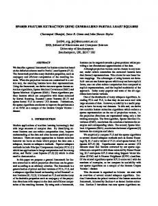
than those from the structured sparse method and SVM(lin). This is due to the nonlinear characteristics in the hyperspectral data. However, in the case of KSC data with 3D-DWT features, group LASSO performs the best. Thirdly, on KSC data, the structured sparse method is better than SVM(lin) and is close to SVM(rbf) in accuracy. However, its computational cost is less than SVM(rbf) because it is a linear solution. To illustrate the effectiveness of the feature selection step of the proposed method, Fig. 2 shows the results on classification accuracies versus sparsity. In the figure, the sparsity of the model is displayed in the blue curve, which is controlled by λ. We used the selected features as the inputs to SVM(rbf) so as to investigate the validity and discriminative power of the selected features. It can be seen that SVM(rbf) with selected features can produce close or better classification results than using all features. This observation suggests that the feature selection by structured sparse method is very effective, which can reduce feature dimensions while preserving the discriminative ability of the features. 5. CONCLUSIONS In this paper, we applied structured sparse model to feature selection and pixel classification for hyperspectral imagery. For these purposes, a logistic group LASSO model with 3DDWT based texture features were developed. This method allows integration of the feature selection and classification steps into a unified model by minimizing the combined empirical loss and penalization on sparsity while taking into account the structure of the input features. We have illustrated the advantages of this method on real-world data and compared our method against raw spectral features based sparse model and SVMs. 6. REFERENCES [1] Y. Qian, F. Yao, and S. Jia, “Band selection for hyperspectral imagery using affinity propagation,” IET Computer Vision, vol. 3, no. 4, pp. 213–222, 2009.

0.75

Lasso SVM(rbf) with selected features Sparsity 4

5

6

7

8

λ=0.5x

(c)

9

10

11

0 12

0.75

0.7

0.2 Group Lasso SVM(rbf) with selected features Sparsity 4

5

6

7

8

9

10

11

0 12

λ=0.5x

(d)

Fig. 2. Results on AVIRIS datasets with 5% sampling rate. (a) Indian Pine with spectral features. (b) Indian Pine with 3D-DWT features. (c) KSC with spectral features. (d) KSC with 3D-DWT features. [2] R. Tibshirani, “Regression shrinkage and selection via the lasso,” J. R. Statist. Soc. B, vol. 58, pp. 267–288, 1996. [3] M. Yuan and Y. Li, “Model selection and estimation in regression with grouped variables,” J. R. Statist. Soc. B, vol. 68, pp. 49–67, 2006. [4] P. Zhao, G. Rocha, and B. Yu, “The composite absolute penalties family for grouped and hierarchical variable selection,” The Annals of Statistics, vol. 37, no. 6A), pp. 3468–3497, 2009. [5] L. Meier, S. Geer, and P. Buhlmann, “The group lasso for logistic regression,” J. R. Statist. Soc. B, vol. 70, pp. 53–67, 2008. [6] P. Tseng, “Convergence of block coordinate descent method for nondifferentiable minimization,” J. Optim. Theory Appl., vol. 109, pp. 475–494, 2001. [7] X. Zhang, N.H. Younan, and C.G. O’Hara, “Wavelet domain statistical hyperspectral soil texture classification,” IEEE Trans. Geosci. Remote Sens., vol. 43, no. 3, pp. 615 – 618, 2005. [8] “AVIRIS NW indiana’s indian pines 1992 data set,” http://dynamo.ecn.purdue.edu/biehl/MultiSpec. [9] J. Ham, Y. Chen, M. Crawford, and J. Ghosh, “Investigation of the random forest framework for classification of hyperspectral data,” IEEE Trans. Geosci. Remote Sens., vol. 43, no. 3, pp. 492–501, 2005.