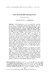
Structured Volume Decomposition via Generalized Sweeping

1

Structured Volume Decomposition via Generalized Sweeping Xifeng Gao, Tobias Martin, Sai Deng, Elaine Cohen, Zhigang Deng, and Guoning Chen Abstract—In this paper, we introduce a volumetric partitioning strategy based on a generalized sweeping framework to seamlessly partition the volume of an input triangle mesh into a collection of deformed cuboids. This is achieved by a user-designed volumetric harmonic function that guides the decomposition of the input volume into a sequence of 2-manifold level sets. A skeletal structure whose corners correspond to corner vertices of a 2D parameterization is extracted for each level set. Corners are placed so that the skeletal structure aligns with features of the input object. Then, a skeletal surface is constructed by matching the skeletal structures of adjacent level sets. The surface sheets of this skeletal surface partition the input volume into the deformed cuboids. The collection of cuboids does not exhibit T-junctions, significantly simplifying the hexahedral mesh generation process, and in particular, it simplifies fitting trivariate B-splines to the deformed cuboids. Intersections of the surface sheets of the skeletal surface correspond to the singular edges of the generated hex-meshes. We apply our technique to a variety of 3D objects and demonstrate the benefit of the structure decomposition in data fitting. Index Terms—Volume decomposition, hexahedral structure, sweeping

F

1

I NTRODUCTION

In a variety of computer graphics and engineering applications such as physically based deformation or free-form deformation, volumetric representations are often required. Among many different types of volumetric mesh representations, because of the better convergence properties [3] and more space efficiency [4], structured representations are often preferred over unstructured representations, such as tetrahedral meshes [5]. The tensor product nature of a structured representation allows the convenient imposition of a simulation basis with a higher derivative smoothness between elements of the volumetric mesh. This means that each individual basis function spans smoothly across multiple elements, which results in visually smoother results. Finite element representations, which possess these properties can yield better numerical results for a variety of applications in engineering (e.g., see Ringleb flow simulation in [6]). Given a hex-mesh, its coarsest version can be obtained by merging neighboring elements without crossing extraordinary (or irregular) edges (i.e., edges that have other than 4 elements incident on it) and the separation surfaces starting from these edges. We refer to this coarsest hex-mesh as the base complex [7], or the structure of the hex-mesh, which is constructed from the irregular edges in the mesh. The inset images in Figure 1 provide the base complexes of the corresponding hex-meshes for the bunny model. The number of hexahedral components in the base complex is • Xifeng Gao, Zhigang Deng, and Guoning Chen are with the Department of Computer Science, University of Houston. • Tobias Martin is with ETH Z¨urich. • Sai Deng and Elaine Cohen are with the School of Computing, University of Utah.

determined by the number of irregular edges and how they are connected. If not treated carefully, a large number of components can result – an issue known as the misalignments among the extraordinary edges [1], [7]. A similar problem has been discussed in surface quadrangulation [8]. Large number of components may pose challenges to the subsequent computations on the corresponding hex-meshes, such as high order spline fitting [9] or using higher order smoothness simulation bases. This is because in applications that use higher order representations, a C 2 B-spline basis can be fitted to each component (not each element). However, in general, only C 0 continuity can be achieved across the boundaries of neighboring components. More components means that the extent of each C 2 continuous region is diminished. In addition, for a hex-mesh with too many components, it may contain some quite small or narrow components. Each of the small components will need to be subdivided multiple times (e.g., see a highlighted component near the boundary in Figure 1c) to get enough number of samples along each of the three parameterization directions, so that the higher-order basis function can be fitted. However, doing so will mean that its neighboring components have to be subdivided accordingly, leading to a very fine mesh with many elements if T-junctions should be avoided. This up-sampling process increases the number of elements in multiples of the original size of the hex-mesh, which makes a fast computation more difficult to achieve. Therefore, fewer components (i.e., a simpler base complex) are desired for the task of spline fitting. However, existing methods [1], [10], [11], [12], [13], [14], [15] cannot guarantee that a hex-mesh with simple structure is generated due to the misalignment issue (Figure 1b-c). Besides the importance of the simplicity of the global structure, given a set of simulation constraints, users may prefer a meshing orientation that is aligned with the anisotropic property of the simulation [16]. However, to date none of

2

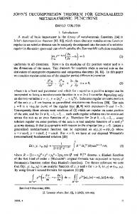
(a) Our4method

(b) SRF4[Li4et4al.42012]

(c) L1-Polycube4[Huang4et4al.42014]

Fig. 1: The hex-meshes of a bunny model. (a) our method has 18 hexahedral components, (b) the SRF method [1] has 259 components, and (c) the L1-Polycube method [2] has 422 components. The corresponding base complexes of these meshes are shown in the inset images, respectively. Green dots are the corners of the individual cuboids and the black lines are their edges. Note that some of the cuboid corners are extraordinary points, others are regular and introduced to avoid T-junctions.

the existing techniques in the literature allows practitioners to efficiently generate a hex-mesh with controllable orientation. In this paper, we introduce a new volumetric decomposition technique for the generation of a simple and predictable structured hex-mesh. In our representation, we emphasize the creation of as few as possible hexahedral components to reduce the number of extraordinary edges (Figure 1a), while allowing the orientation of the structure to follow a user desired direction (kitten and bunny in Figure 11). Given an input surface/tetrahedral model, our pipeline employs a generalized sweeping strategy to decompose the volume enclosed by the input polygonal surface into a sequence of 2-manifold level sets based on a user-specified 3D harmonic function. This effectively reduces the complex 3D spatial partitioning problem to a simpler partitioning problem in 2D. The final 3D partitioning strategy is constructed via matching the 2D solutions over the adjacent level sets. The obtained level sets in our method are typically curved, which differentiates our method from planar sweeping strategies [14], [15]. Note that global structures of all the hex-meshes generated using our approach are well aligned. This property is guaranteed, since the global structure of a hex-mesh produced by our approach is controlled by the 3D skeletal structure without any misalignment through our sweeping strategy. In particular, we make the following contributions. 1. We introduce the concept of a 2D skeletal structure. This structure has a simple quadrilateral configuration that reflects the primary characteristic of the 2D region. Figure 15a provides an example of such a structure (highlighted by different color components) in the cross section of a deformed torus. 2. We present a robust and automatic algorithm to extract the four corners of a 2D shape based on its medial axis. In comparison with corner placements found by following gradient lines of the surface harmonic function [11], our corner extraction can better align the hex-mesh structure with the surface features along the sweeping direction.

3. We introduce a skeletal surface to compute a structured volumetric decomposition. It is constructed by matching and connecting the 2D skeletal structures through adjacent level sets with special attention paid to bifurcations. The resulting surface (Figure 1a) not only provides a valid all hexahedral partitioning strategy for the volume, but also serves as a user-controllable representation of the extraordinary structure for the subsequent 3D global parameterization.

2

R ELATED W ORK

A wide variety of methods exist to create a hexahedral mesh from an input triangle mesh [17]. However, since the aim of our method is to produce a representation which decomposes an object into a set of large hexahedral pieces, in the following we focus on methods which have the potential to produce such a result. Polycubes: Polycubes allow the decomposition of an object into a set of larger hexahedral pieces. However, the quality of the resulting hexahedral representation strongly depends on the placement of polycube corners on the input triangle mesh. This challenging process has received a lot of attention recently [10], [18]. Automatic methods are usually difficult to control. Livesu et al. [19] and Huang et al. [2] introduced Polycuts and L1-Polycubes to improve the corner configuration of the conventional polycube. However, control of the interior structure of the volume is still missing. Recently, Li et al. [11] extended the conventional polycube to a generalized polycube (or GPC), which enables the curved cuboid representation of the elementary sub-volumes decomposed via shape analysis. While this enables the polycube map approach to be applied to more complex objects, the corners of the GPC are located on the surface, leading to degenerate elements (negative Jacobian) around the corners. The sub-volumes decomposed using our framework are curved cuboids, which is similar to GPC. We address the boundary degeneracy by finding the

3

correspondence of the boundary corners of these cuboids in the interior of the volume. Cross field guided approaches: Cross fields (or frame fields) have been proven useful to assist the placement of quadrilateral elements when quadrangulating a triangular mesh [20], [21], [22], [23], as it provides consistent local frame information everywhere in the domain to guide the orientation of parameterization. Nevertheless, it is not clear on how to extend these methods from quadrangulation to hexahedralization. Huang et al. [24] proposed a first solution to creating a boundary conformal 3D cross field via an expensive optimization. Due to insufficient control on the types of the singularities in the cross field, their approach cannot be guaranteed to generate an all-hex mesh. Nieser et al. [12] pointed out that only 10 types of singularities can lead to a valid all-hex mesh. Recently, Li et al. [1] introduced the Singularity Restricted Field (SRF) that converts a general 3D cross field to one that contains only these 10 types of singularities. After regularizing the SRF and fixing degeneracies, high quality hex-meshes can then be generated using the CubeCover technique [12]. A similar work by Jiang et al. [13] also aims to derive a restricted cross field from some initial cross field using similar singularity operations as in [1]. The obtained cross field is then used to compute a parameterization by solving a mixed-integer problem. Both Polycubes and cross field approaches may generate hex-meshes with degenerate boundary points (i.e., zero Jacobian). They apply an additional step, called padding, to relocate the degenerate boundary points into the interior of the volume. However, this is achieved by simply adding an additional layer of hex-elements, which may introduce additional small hexahedral components to the structure. This limits the order of splines that can be fitted in this layer. Our approach addresses this limitation by finding the correspondence of the surface corners in the interior of the volume so that sufficient samples can be placed between the boundary and the interior structure (see Figure 15). Sweeping strategy and mid-structure for hex-meshing: There are other hex-meshing techniques that are based on sweeping and paving, such as the unconstrained paving and plastering [14] and a skeleton-based sweeping [15]. However, those techniques require the cross sections to be planar, and the structure of the obtained hex-meshes is uncontrollable. Therefore, they are typically suitable for the meshing of CAD models rather than more organic appealing 3D models. In contrast, our generalized sweeping strategy is guided by a harmonic field, leading to curved cross sections. And the introduced skeletal surface provides a means for explicit control on the structure of the generated mesh. The idea of utilizing a simplified mid-structure of an input model to assist the generation of hexahedral meshes has been explored by [25], [26]. Note that our skeletal surface is not a mid-structure in the sense of a medial axis.

3

OVERVIEW OF O UR A PPROACH

Before presenting our method, we define the notation used in the paper. We use calligraphic letters for objects in R3 , for example, L denotes a 3D level set generated by our sweeping process (see below), T denotes a set of triangles in 3D space, and P denotes a 3D point. Superscripts refer to level set identifications, while subscripts refer to the identifications of the geometric objects at a certain level set. For instance, Pji represents the j th point on the ith level set. Regular letters, such as L, Q, and p, represent objects in R2 . Let (T , VT , CT ) be a closed 2-manifold in 3D space represented by a triangle mesh, where T is the set of triangles, VT is the set of vertices, and CT is the connectivity of the mesh. The volume enclosed by T is filled with tetrahedral elements using an automatic tet-meshing method, such as Tetgen [27]. In Tetgen we use 0.5% of the diagonal of the bounding box of the model to create tetrahedral elements whose boundary triangles have similar sizes as the remeshed input. Let (H, VH , CH ) define a tetrahedral mesh, where H is the set of tetrahedra, VH is the set of vertices defining the tetrahedra, and CH is the connectivity of the tetmesh. Figure 2 illustrates our pipeline that generates the structured mesh from the given input triangle mesh T , by executing: 1. Compute a harmonic function hu (x, y, z) on H based on user-specified constraints (Figure 2a). Decompose H into a sequence of non-planar level sets Li (Figure 2b). Li is flattened to a 2D level set using least-square conformal mapping (LSCM) [28]. Let fi : Li → Li be the resulting bijective mapping function. (Sections 3.1 and 3.2) 2. Extract four corners for each level set Li and align them with the adjacent level sets. A skeletal 2D structure Qi of Li is constructed by projecting each of these corners to the interior (Section 4). The inner structure Qi of Li is obtained via fi−1 (Qi ) (Figure 2b). 3. Iteratively match Qi through adjacent level sets and connect them to form a 3D skeletal surface S (Figure 2c) (Section 5). 4. Compute the 3D parameterization induced by the volumetric partitioning provided by S. This parameterization can be used to generate structured all hex-meshes (Figure 2d) without T-junctions. Note that there are four user-specified parameters in our pipeline: The resolutions along U , V , W directions (Section 6) and the number of level sets for the sweeping (Section 3.2). The remaining parameters mentioned in our paper are set as either constant values or constant ratios, and do not require model specific tuning. In the following two sections we describe the first step in this pipeline. Then, the remainder of the paper is fully dedicated to the subsequent steps.

4

(a) Design harmonic function Extract 2D level sets.

(b) Extract corners of Compute inner structure .

(c) Construct skeletal surface .

(d) Generate all-hex meshes

Fig. 2: The pipeline of the proposed method. (a) A generalized sweep guided by a user-specified harmonic function; (b) corner extraction and inner structure construction in 2D parameter space; (c) the skeletal surface constructed by matching the 2D structure; (d) the multi-resolution hex-meshes generated based on the structured decomposition.

3.1

Computing 3D Harmonic Function

A scalar function u(x, y, z) (in the remainder of the paper, denote as u for simplicity), defined on H, is harmonic if it satisfies Laplace’s equation, i.e., ∇2 u = 0. Here, u satisfies the maximum principle, i.e., it only exhibits maxima and minima at user-specified locations on H. This makes it a convenient and highly controllable tool to guide a meshing process. It has been used in a variety of mesh generation and volumetric parameterization methods [29], [30], as well as in skeleton extraction methods such as [31]. In this work, the harmonic function u is computed by first discretizing Laplace’s equation using Galerkin’s formulation [32]. The set of vertices VH is decomposed into a set of constrained vertices VB , and a set of free vertices VF for which a solution is sought. In our framework, the user has full control over u by defining VB through vertex selections directly made on H. As an example, Figure 11 illustrates two harmonic functions on the genus-1 kitten and bunny models, respectively, which creates two different yet valid structured hex mesh representations. u is seen as a sweeping strategy as it is used to decompose the object into a set of slices, where a slice is a level set of u. This step is discussed in more detail in the following section. Note that if the resulted slices contain holes (non-multi-disk type), the user is prompted by our system to specify a different set of critical points to compute a new harmonic function. 3.2

Decomposition of H

Given the harmonic function u, the object is decomposed into a set of slices Li . A slice Li (Figure 2b), at value ui ∈ R is the level set satisfying u = ui . Li is extracted using marching tetrahedra [33]. Depending on the choice of VB and resulting saddle points [34], Li can consist of multiple disjoint non-planar 2-manifolds represented as triangle meshes with boundaries [35]. If slices are placed such that every triangle in T is intersected by at least one slice, all features will be guaranteed to be present in T . However, in this work, ui is a

Mi

p1

p4

d

w

p2

p3 L

i

p4

Qi

p1

q1

q4

q2

q3

p2

(a)

p3 (b)

Fig. 3: 2D structure extraction. (a) Flattened level set Li with its bounding box guided by its medial axis M i and boundary corners pj . This bounding box is different from the one (the light green box) obtained by performing PCA on Li . (b) The corners of Qi are found on the iso-contour by the one-to-one mapping between pj and qj . The offset distance d = dm /3, where dm is the maximum scalar value of a distance field computed from B i .

uniform sample on the range of the harmonic function u. This uniform sampling strategy allows the user to control the number of slices more conveniently. Except for some simple models, a dense cutting with about 500 slices is typically used for the examples shown in the paper. This high number of slices assures capturing all the features present in T . A more advanced slicing approach could be adopted (e.g., [36]). While it may improve accuracy to certain extent, it is computationally more expensive. Finally, each slice Li is flattened using the CGAL [37] implementation of LSCM [28]. The boundary of the flattened Li is approximated with a periodic B-spline curve using the method proposed in [30].

4

2D S KELETAL S TRUCTURE

In this section, we provide the definition and computation of the inner structure of a planar level set Li . Consider a 2D region LiSwith closed boundary B i = ∂Li . N −1 A segmentation strategy j=0 Sji of B i partitions B i into N segments separated by N boundary points, pij ∈ B. An inner structure Qi is defined as a polygon with N vertices in the interior of Li whose corners qij map one-to-one to the boundary separating points pij . Qi represents the characteristic of B i , e.g., the primary orientation or curvature extrema with controllable complexity. For simplicity of the

5

subsequent matching and the requirement to produce an all-hex configuration, in this work, we set N = 4. As described previously, the most challenging part of extracting Qi is to determine the locations of its corners. We adopt a two-stage approach to determine the corners of Qi . First, we determine the locations of the corners on B i based on its configuration. Second, we project the obtained corners on B i to the interior of Li without ambiguities in the gradient direction of a distance field computed with B i being the zero level set. Figure 3 illustrates this process.

4.1

Corner Point Extraction

Given Li we follow the approach in [36] to compute its medial axis. The medial axis is the locus of centers of maximally inscribed circles that are tangent to the boundary. The contact points of each maximal circle with the boundary curve are called foot points. The computed medial axis for Li is effectively denoised because it is computed from a smoothed curve. It can be further simplified with an area based filtering. Figure 4a shows a slice of a twisted U-shape model and its simplified medial axis. For each branch of the medial axis, if the area (for example, the dotted area in Figure 4a) bounded by its branch point, corresponding foot points and the boundary between foot points is smaller than 1/10 of the area of the slice, then we remove this branch. At this moment, if the simplified medial axis has only two end points, then we trace from the end points to the internal points, until the separation angle between the foot points of the current medial axis point is larger than a predefined value (we use 120◦ in this work). The corner points are the foot points of the traced medial axis points. Otherwise there are more than two end points in the medial axis, and in this case we compute a principal component analysis (PCA) of the medial axis curves, to obtain the dominant direction from which to extract the bounding box. Once the bounding box is computed and the corners are mapped onto the flattened slices, the corner points are inversely mapped onto the original (non-planar) slices. Note that the bounding box of the medial axis may not produce desirable corners. In addition, for more symmetrical slices (e.g. circular shape), the orientation given by the PCA is less reliable. The corners of both situations will be adjusted by a smoothing process discussed next. 4.2

Corner Point Matching Over Level Sets

After the corner points at individual level sets are extracted, they are matched between adjacent 3D level sets for the construction of a 3D inner skeletal surface (Section 5). To determine the correspondence between corners at adjacent level sets, we employ a distance based greedy algorithm, modified by using the ratio of the eigenvalues of the PCA on the medial axis. If the ratio (λi in Algorithm 1) is larger than a specified , each corner is matched to its nearest corner in the previous slice. Otherwise, the corners are

foot points branch point

L i+1 end point corner points seperation angle

(a)

Li valid match invalid match

(b)

Fig. 4: Corner extraction and matching. (a) illustrates the corner (i.e., green dots) extraction using a simplified medial axis (the dark red curve) of a slice of a twisted U shape. The simplified medial axis consists of one branch point (blue dot) and three end points (orange dots). Foot points of the branch point are shown as black dots. (b) shows the matching of the corners between two adjacent level sets with a splitting bifurcation. The shaded area shows a highly distorted quad.

recalculated by finding the points on the current slice that are closest to the corner points in the previous slice. Doing so enables us to avoid big matching jumps, by skipping the nearly symmetric slices with the ratio of eigenvalues close to one. In some symmetric slices, e.g., the slices crossing the pectoral fins of the dolphin model, by changing , users may control whether to put corner points close to shape features or away from them to get smoother results. Figure 5a shows the corners on the surface of a dolphin model with  = 1.5 and 2, respectively. For all models shown in this work,  = 1.5 was used. Algorithm 1 provides pseudo-code for the extraction of the corner points on each level set and their matching over adjacent slices. Four or more chains can be computed in this way. Each chain that is formed by the matched corners is shown in the same color in Figure 5. When a bifurcation occurs, emphasis is placed on the continuity of the adjacent chains from the previous levels wherever possible to maintain good spacing of the corners. For example, in Figure 4b, the invalid match (shown by the red dash line segment) loses the continuity. The adjacent chain in the previous slice becomes non-adjacent after bifurcation. The correct matching is shown by the cyan line segments. However, forcing continuity of chains can lead to distortion. As shown in Figure 4b, the matching line segments in the right are almost tangent to Li+1 . Thus, the quad-region (shaded) formed by these four corners is skewed, leading to distortion in the subsequent hex-mesh. This is due to the independent nature of the extraction of the corners at their individual level sets and the rapid change of the surface features along the gradient of the harmonic function. We introduce a smoothing process to remove this noise and reduce distortion. For each chain, we use the corresponding vertices on each Li to define a Schoenberg Variation diminishing spline approximation (SVDSA) [38], γi0 (t). We then find the closest points on each slice to the curve. Next, we use the new points to define the control points of the next iterated SVDSA, γij (t). If there is significant noise that results in sudden zig-zags in the original corner curves, this

6

Algorithm 1: Pseudo code of corner point extraction and matching

Algorithm 2: SVDSA Input : {Li }, {γi } Output: {P i }, {γi } foreach γ in {γi } do γ0 ← new B-spline curve; foreach control point Pci in γ.{control points} do s ← evaluate γ at the node value related to Pci ; P i ← closest point on ∂Li to s; γ0.{control points} ← P i ; γ ← γ0

i

Input : a set of slices {L }, , n Output: corner points {Pji } foreach L in {Li } do {mj } ← simplified medial axis of L; CM ← covariance matrix of {mj }; λ1 , λ2 ← eigenvalues of CM (λ1 is the larger eigenvalue); v ← the eigenvector associated with λ1 ; if there are two end points in {mj } then trace from end points to m1 and m2 with the separation angle > 120◦ ; pi1 , pi2 , pi3 , pi4 ← foot points of m1 and m2 ; else Bx ← bounding box of L in direction v; pi1 , pi2 , pi3 , pi4 ← the four closest points on ∂L to four corners of Bx ; p λi ← λ1 /λ2 ; map {Li } and {pij } back to original space of Li ; foreach L in {Li } do if λi <  then P i ← closest point on ∂Li to P i−1 ; match {Pji } across the slices and use them as the control points {Pcj i } to generate B-spline curves {γi0 }; for j=1 to n do ({P i }, {γij }) ← SVDSA({Li }, {γij−1 })

Saddle point

L i+1 L

Q

Q i+1,0

P0

Q i+1,0

Qi

Li L

i-1

P0

P1

P0

R0

(b)

Q i+1,1

V

U

R1

Qi

(a)

L i+1

Q i+1,1

Q i+1,0

P1

Qi

i

i+1,1

P1

Q i+1,1

Q i+1,0 Qi P1

Q i-1

P0

(d)

(c)

Fig. 6: Illustration of bifurcation handling. (a) illustrates that a level set Li splits into two components in Li+1 , so does the corresponding inner structure. (b) demonstrates the two unmatched patches (i.e., the shaded regions) are mapped to a saddle patch formed by the separatrix segment at Li , (c) shows the connection between Qi and Qi+1,0 and the hex element formed by the last level set and the surface, i.e. the cap. Note that P0 P1 has been pushed down along the inverse gradient of harmonics function to eliminate the degeneracy, (d) illustrates the matching of the parameterizations of Li−1 , Li , and Li+1 guided by the inner structure. surface extraordinary nodes (valence 6)

(b)

(a) ε=1.5

ε=2

before

after

Fig. 5: The corners of the dolphin model (left) with  = 1.5 and  = 2, respectively. The corners of the kitten model (right) before and after 100 smoothing steps. Corners are represented as colored dots. The harmonic function for kitten is designed by cutting the handle, where the vertices of the (two) cutting areas are set to minimum (w = 0) and maximum (w = 1), respectively.

acts as a low pass smoothing filter to the chains. The new set of control points have reduced wiggles. Here the upper index indicates the number of iterations of this process. This process is fast and can be carried out as necessary to create smoothed corner curves, suitable for offsetting inwardly to create the inner volume structure. Algorithm 2 provides the pseudo-code of this smoothing process. Figure 5b shows the chains of corners of the kitten model before and after smoothing.

(a)

(b)

interior extraordinary nodes

Fig. 7: Bifurcation handling for the sculpture model. (a) shows the bifurcation of the sculpture model (zoom-in view shows the separatrix crosses the saddle point), (b) visualizes the obtained hex mesh with the line structure being highlighted. The red nodes are the extraordinary nodes in the generated hex mesh.

4.3

Computing the Corners of the Interior Structure

To obtain the corners of the inner structure Qi , we first compute a distance field with the distance value as 0 for boundary vertices. Next, we compute an iso-contour in the interior of Li corresponding to a distance value d based

7

on the obtained distance field. The one-to-one mapping between the boundary and the interior contour is guaranteed because 1) we can always locate the four interior corners by following the gradient directions of the distance field on Li ; 2) boundary and interior contour are partitioned into four pieces by the four corners. For each piece of the interior contour, the to be matched interior points can be found by accumulating chord length parameterization using the same ratios as boundary curve. As Li is the flattening of Li via the bijective mapping fi , Qi can be recovered from Qi via fi−1 .

5

3D S KELETAL S URFACE

After constructing the inner structure Qi for each individual level set Li , we now describe how to match the inner structure Qi through adjacent level sets to form a partitioning surface S (in 3D) (see Figure 9 for some examples), which is referred to as the inner skeletal surface. Based on the matched corners determined by Algorithm 1, we identify the corresponding matched edges of Qi and Qi+1 , which are connected to construct a quadrilateral face. The configuration of the boundary surface and the selection of the harmonic function may cause bifurcations that split a preceding level set Li into multiple connected components in the current level set Li+1 , or vice versa, e.g., at the base of the two branches of the sculpture model (Figure 7a). These bifurcations correspond to the saddle points in the harmonic function, and their identification can be performed automatically and robustly. Consequently, following the sweeping direction, the structure of Qi also undergoes splitting or merging to accommodate such topological changes. Section 5.1 details the handling of the splitting scenario. The merging case is handled analogously. n-way bifurcations are divided into a sequence of 2-bifurcations and are handled individually.

5.1

Q i+1,0

L

Q i+1,1

i+1

Li

Qi

(a)

before

(b)

after

Fig. 8: Improvement at bifurcations. (a) illustrates the process that splits the line segment across the saddle into two. Three hexahedral components are generated instead of two. Different colored lines indicate their correspondence relation. (b) shows the result of the kitten model before and after the bifurcation improvement process.

by the curve R0 R1 and the edges P0 P1 , R0 P0 , and P1 R1 can then be mapped to the two unmatched components (the shaded regions in Figure 6c). In practice, a short segment across the saddle point on the surface can be obtained by computing two separatrices starting from the saddle point along the incoming (outgoing) gradient flow direction for a splitting (merging) bifurcation. The computation of these separatrices is terminated when they reach the level set Li (Li+2 for merging). Second, pushing down P0 P1 along the negative harmonic gradient direction as long as P0 P1 is still above Li−1 (Figure 6c), since P0 P1 R1 R0 is a degenerate element as the four corners are almost collinear. Third, by creating a saddle patch, computing the mapping between Qi and Qi+1 . However, this solution leads to a T-junction configuration when considering Qi and Qi−1 since Qi has been split into two components in the previous process. See Figure 6d for an illustration. Specifically, if a line segment enclosed by the shaded ellipse is not added in Li−1 , a T-junction configuration occurs. More discussions are provided on this issue in Section 6. Figure 7b shows the generated hex mesh for the sculpture model at the bifurcation. The structure of this mesh formed by the irregular edges is highlighted in blue. The colored dots are the intersections of the irregular edges with the cutting planes.

Matching of Qi Across Bifurcations

Figure 6a depicts a case of splitting a level set. During this change, Qi of Li splits into two components, Qi+1,0 and Qi+1,1 in Li+1 . There is no one-to-one mapping between the sub-regions of Li and Li+1 partitioned by Qi , Qi+1,0 and Qi+1,1 , respectively. Specifically, an interior edge, P0 P1 (the red line segment in Figure 6b) that splits Qi into two components must be mapped to two respective edges of Qi+1,0 and Qi+1,1 . In addition, if mapping different components of the two level sets as indicated by the colors shown in Figure 6a, two unshaded regions of Li+1 do not have a correspondence. This is addressed by performing the following steps: First, computing a small segment on the surface that crosses the saddle point and intersects with Li at R0 and R1 , respectively (i.e., the red curved segment in Figure 6b). A new section, referred to as a saddle patch and formed

Bifurcation improvement The above basic bifurcation handling introduces a valence-6 extraordinary node at each side of the bifurcation on the boundary quad mesh (orange dot in the left figure of Figure 8b). This may lead to large distortion in elements at bifurcations whose neighborhood is relatively flat. To lessen the distortion, instead of associating the two unmatched components to a section across the saddle point as shown in Figure 6c, we map them to two sections as shown in Figure 8a. This splits the valence-6 (the number of neighboring hexahedral elements) extraordinary point into two valence-5 nodes (Figure 8b). This adds an additional component at the bifurcation (e.g., the purple region in Figure 8a). Since the gradient of the harmonic field is curl-free, by transferring this configuration down (splitting bifurcation) or up (merging bifurcation) following the sweeping direction, T-junction configurations can be avoided. Note that this improvement is not required

8

and can be selected by the user according to the surface characteristics around the bifurcations. We have applied this improvement to the kitten, fertility, blade, and rocker arm models in our experiments. 5.2

Properties of the Skeletal Surface S

Figure 9 (top row) shows the skeletal surfaces S of a variety of 3D objects computed using the aforementioned framework. As explained earlier, the corners of the inner structure Qi correspond to the extraordinary points of a 2D parameterization derived by Qi . By matching Qi over adjacent level sets to construct S, the extraordinary points in 2D now form line structures in 3D as indicated by the intersections of different surface sheets (with dark blue and red in Figure 9) of S. These line structures, referred to as the extraordinary edges, correspond to the irregular edges (or singular edges by Nieser et al. [12]) with valence not equal to four in the obtained hexahedral mesh. The extraordinary edges in S can start and end at either some extraordinary nodes in the interior of the volume or on the exterior surface. Specifically, the extraordinary lines start and end on the boundary surface when a component of the level set either is born or vanishes (e.g., the four red points on the top of the shaded surface in Figure 6d). In the meantime, the extraordinary lines meet at the extraordinary nodes at the bifurcations. Figure 6f illustrates this. The two red points (corresponding to P0 and P1 in the previous steps) are valence-5 extraordinary nodes (i.e., there are five edges incident to each of them) in the hex mesh. In the meantime, the two orange points (corresponding to R0 and R1 ) are valence-6 extraordinary nodes on the boundary quad-mesh.

(a)

(b)

(c)

Fig. 9: Inner skeletal surfaces S and base complexes CB of the twisted U (a), kitten (b), and hand (c). The top row shows the skeletal surfaces with the singular line structure being highlighted (i.e., black curves). Red sheets show the interior surfaces, while blue sheets are the separation surfaces connecting the interior surfaces and the exterior boundary surfaces. The bottom row shows their corresponding base complexes. Nodes and edges are the corners and edges of the cuboids, respectively.

The base complex CB of the subsequent hex-mesh can be derived from the skeletal surface S. Specifically, if the

sweeping does not involve bifurcations, S and CB have a one-to-one mapping (Figure 9a). If bifurcations exist, the skeletal surfaces may contain T-junctions because of the way bifurcations are handled(see Figure 6 and Section 5.1). Nonetheless, their corresponding base complexes do not contain T-junctions (Figure 9b and 9c) as a separation surface will be added at T-junctions to enforce an all-hex configuration in the base complex structure. Therefore, the nodes in the base complexes (green dots) consist of both, extraordinary points and regular points.

6

PARAMETERIZATION AND H EX -M ESHING

This section describes how to compute a seamless 3D parameterization and induce hex-meshes with large hexahedral components, after constructing S. Parameterization: Similar to computing S, one parameterization direction w is provided by harmonic function u(x, y, z). The computation of a 3D parameterization can be simplified by two steps: 1) compute a 2D parameterization f i of Li based on its Qi ; and 2) match f i and f i+1 to obtain a 3D parameterization F. p1

q1 q2

p2

Qi

p4

q4

q3 p3

Fig. 10: Iso-lines for 2D parameterization.

S The 2D parameterization, f i = j fji of Li , consists of five patches. Each patch Lij is triangulated and can be mapped to a rectangular region via fji : Lij → [0, n] × [0, m] ⊂ R2 . To compute fji , we apply Floater’s mean value coordinates [39] to calculate the u and v values for each vertex of Lij . To guarantee a continuous parameterization across the boundaries of different patches, we classify the parameterization directions into three groups, i.e., the red, green, and blue dotted curves, respectively, as shown in Figure 10. Given the 2D parameterizations for all level sets, a 3D volumetric parameterization can be constructed accordingly. For the adjacent level sets without bifurcation, the correspondence of their 2D parameterizations is one-toone. When a bifurcation occurs, we match f i−1 , f i , and f i+1 via the correspondences between their inner structures obtained in Section 5.1 as illustrated by Figure 6e. In this case, the bifurcation occurs between level sets Li and Li+1 . To build the correspondence between f i and f i+1 (composed of f i+1,0 and f i+1,1 ), we make use of the two sides of the saddle patch, which splits the inner structure Qi (and f i ) into two components. The segment crossing the saddle is mapped to the line segment P0 P1 parallel to the parameterization direction V (red). Its perpendicular direction is denoted as U (blue), and the integer value of P0 P1 is uP . To avoid a T-junction configuration, we set

9

the numbers of isolines parallel to the U direction to be the same for both f i+1,0 and f i+1,1 . That is, we use the same number of samples along the six red segments (i.e., along V parameterization direction) in both level sets Li and Li+1 , as illustrated by the intersections of the blue isolines with the six red segments (Figure 6e). The matching between f i−1 with f i can be coordinated after the above process to avoid a T-junction configuration. Fortunately, the split of Qi does not introduce a new singular structure at the splitting edge P0 P1 , i.e., both P0 and P1 are still valence4 nodes. Therefore, T-junctions can be avoided by enforcing an isoline to be included in the parameterization f i−1 that has the same integer value uP to the one that corresponds to P0 P1 in f i . This isoline is highlighted by the shaded ellipse in level set Li−1 in Figure 6e. Hex-meshing: The hex-mesh is constructed in two steps. First, an all-quad mesh is obtained by following the isolines of the integer values of the 2D parameterization for each level set. Second, all the quad meshes are matched in the same fashion as the construction of the 3D parameterization. The numbers of samples, nU , nV , and nW , are user-provided parameters that control the resolution of the hex-mesh. Since we cut densely in the first step, when a coarse hex mesh is preferred, we merge hex elements that are in two neighboring levels to keep an approximate regular aspect ratio of edge length in three parameterization directions. To improve the quality of the obtained mesh, we perform Laplacian smoothing on both the interior and exterior vertices and then optimize the mesh using the technique by Knupp [40]. Note that since the boundary extraordinary points are explicitly placed on the surface regions that correspond to the first and last slices (see the four red dots at the top of the surface in Figure 6c), a process similar to the padding [41] may be carried out to offset these extraordinary points to the interior. However, this process is optional and only used to improve the element quality in those regions if needed. Although all the hex-meshes tested in this work have positive Jacobians, we cannot guarantee that our pipeline can always generate hex-meshes without inverted elements.

7

with Intel i7 2670QM 2.2GHz CPU and 8GB RAM. A detailed report on timing and mesh quality is provided in the supplemental material. In the following, we discuss our results with respect to control, comparison with existing methods, element quality, and volumetric B-spline fitting. In Figure 11, the kitten model is meshed from two different choices of harmonic functions, one with bifurcation and one without bifurcation. The blue arrows indicate the directions of the harmonic functions. Similarly, for the bunny model, both meshes have their maxima at the tips of the ears (in green). While the upper bunny has its single minimum at the tail (in red), the lower bunny has its whole base fixed as minimum (not visible from the given view). These examples demonstrate that our pipeline outputs valid meshes for different user-specified harmonic functions. The choice of harmonic functions is mostly application-specific. For instance, the problem of establishing continuity among elements given the kitten model without bifurcation is significantly reduced, as one does not have to deal with a bifurcation point during a higher-order spline fitting process. A sweeping strategy could be derived automatically based on shape analysis of the input object. However, this is beyond the scope of this work. Higher genus models: We apply our method to the fertility model (Figure 12) to demonstrate that our pipeline can be used for higher genus models. The left-most image is the base complex of these meshes, while the right most shows the Jacobian visualization and histogram of the Jacobian distribution. This object is meshed based on a harmonic function with two critical points: One minimum (at the back of the mother), and one maximum (at the base opposite to the minimum). This harmonic function results in a sweeping that generates 3-way bifurcations in the level sets, which are handled by splitting 3-way bifurcations to two consecutive 2-way bifurcations (Section 6).

R ESULTS AND D ISCUSSION

We have applied our proposed approach to various models. All the obtained hex-meshes have large hexahedral structure. Figure 11 provides the hex-meshes of a variety of 3D objects with three different resolutions. Hexahedral elements that belong to the same components of the structure of the mesh are shown in the same colors. For all the models shown in this paper, at most 600 slices are used for the cutting, which takes up to 2 minutes to compute. The corner extraction (including medial axis computation) takes one min per slice. The time spent on the generation of hex-meshes ranges from 5 seconds to 2 minutes, depending on the mesh resolution. All timings are obtained on a PC

(a)

(b)

Fig. 13: Results of two CAD models with our method: (a) the rocker arm and (b) the blade. The circle highlights the area with distorted elements in the blade mesh.

CAD models: Methods that output hex-meshes with large structure are often challenged by the complexity of input models. In this context, CAD models are especially difficult to mesh. To demonstrate that our method can be used to mesh a certain class of CAD models, we apply it to the

10

Fig. 11: Different resolutions of the hex-meshes generated for a variety of 3D models. Note that the components with white colors are in the interior, while the others with different colors are at the exterior. 5

4

x 10

3.5

3

2.5

2

1.5

1

0.5

0

0

0.1

0.2

0.3

0.4

0.5

0.6

0.7

0.8

0.9

1

1.0 0.5 0.0

Fig. 12: The result of the fertility. The left-most image shows the base complex; the middle three images show generated hex-meshes with decreasing resolution; and the right-most one shows the Jacobian visualization and the histogram of the Jacobian distribution.

blade and the rocker arm. Figure 13 shows the results. Note that the sharp features of these CAD models are properly preserved by our corner extractions. The element quality of the meshed rocker arm is comparable to those generated by existing methods. Even so, distorted elements can be observed in the areas that the surface normal is almost parallel to the gradient direction of the harmonic field (e.g., the flat region of the blade as highlighted in Figure 13b). This may be addressed by inserting additional extraordinary points in this area in a similar fashion to the extended bifurcation handling shown in Figure 8.

7.1

Comparison With Existing Methods

Comparison with cross field based methods: Figure 1 compares our method with the SRF approach [1]. The structure of the hex-mesh with SRF is guided by the structure of SRF (i.e., the singular graph). However, as pointed out by its authors, the structure of the obtained hex-mesh may not match the structure of SRF due to the parameterization. Furthermore, the extraordinary (or

singularity) points are not always aligned, leading to many small components in the structure. For instance, there are 259 components in the hex-mesh of the bunny using SRF (Figure 1b) while ours has only 18 components (Figure 1a). Figure 14 shows a deformed rabbit model. While this frame field based method fails to find a valid all-hex mesh for this model due to certain global degeneracies in the parameterization [13], our method successfully computes valid hex-meshes with various resolutions. Compare to Polycube based methods: Figure 1 compares our method with the L1-Polycube method [2]. In order to remove polycube corners from the exterior, they are pushed into the interior of the object by adding one boundary layer. While it might be possible to apply this method to a wider range of input models, this offsetting process cannot guarantee to preserve the large polycube structure, and may result in additional T-junctions. Removing them leads to additional smaller hexahedral components. For instance, the bunny model meshed by the L1-Polycube approach has 422 components (Figure 1b) and 580 components with

11

5

x 10 5

x 10

4

x 10 2.5

3.5

12 3

2

10

2.5

1.5

8

2

1

1.5

6

1

4

0.5 0.5

2 0 0

0

0.1

0.2

0.3

0.4

0.5

0.6

0.7

0.8

0.9

1

(0.14,0.93)

0

0.1

0.2

0.3

0.4

0.5

0.6

0.7

0.8

0.9

1

(0.05,0.89)

0

0

0.1

0.2

0.3

0.4

0.5

0.6

0.7

0.8

0.9

1

(0.13,0.90) 4

x 10

2

1.5

1

0.5

0

0

0.1

0.2

0.3

0.4

0.5

0.6

0.7

0.8

0.9

1

(0.67,0.90) 4

x 10

4

x 10

4

x 10

7

16

18

14

16

6

5

14

12 4

12

10

10

3

8 8

2

6 6 4

1

4 0

(a) degeneracies

2 0

0.1

0.2

0.3

0.4

0.5

0.6

0.7

0.8

0.9

2

1

(0.07,0.82)

(b) our approach

0

0

0.1

0.2

0.3

0.4

0.5

0.6

0.7

0.8

0.9

1

(0.11,0.89)

0

0

0.1

0.2

0.3

0.4

0.5

0.6

0.7

0.8

0.9

1

(0.10,0.918) 1.0

Fig. 14: A rabbit model where the frame field based method fails and our method succeeds. (a) Demonstrates the global degeneracy, resulting in a invalid hex-mesh. Red lines are inner singularities and cyan lines are surface singularities, they are processed by using the method proposed in [13], black rectangle shows a global degeneration; (b) our all-hex mesh and base complex.

Polycut, which makes it difficult to establish a smooth basis almost everywhere in the model. In contrast, the structure of the hex-meshes produced with our method is simpler, predictable and controllable. Compare to GPC: With Generalized PolyCubes (GPC) [11], the faces of each cuboid can be curved, which is similar to our representation. However, an important difference is that the edges of the GPC cuboid are obtained by tracing along the gradient of a surface harmonic field, which may follow surface features only by coincidence. Figure 15 shows a comparison of the placement of the corners for the deformed torus with the proposed extraction technique guided by the medial axis of the 2D level sets (a) and the one (b) that aligns the corners by following the gradient of a harmonic function. From the comparison, we see that the one generated by following the harmonic field fails to capture the transition of the surface configuration, leading to the improper orientation of the structure of the obtained hex-mesh, i.e., the structure is not aligned with the anisotropy property of the cross section. Note that the first four corners of the first slice for the harmonic field based approach are extracted using our proposed algorithm. This indicates that only focusing on obtaining the optimal corners at the initial slice is typically insufficient. Furthermore, for all the models, GPC places corners on the boundary rather than in the interior. This is generally avoided by most hex-meshing techniques, especially when dealing with natural shape models, since degenerate elements arise quite often around singularities on the boundary.

(a)

0.5 0.0

Fig. 16: Visualizations and histograms of the Jacobian value distribution of a number of hex-meshes. The red-white-blue color coding is used with red indicating smaller Jacobian values. The numbers show the minimum and average Jacobian values. More information is provided in the supplemental material.

7.2

Element Quality

Figure 16 provides the visualization of the scaled Jacobian values [42] of the meshes shown in Figure 11 with blue denoting Jacobians close to one and red close to zero. The histograms show the distribution of Jacobians for the finest versions of the meshes with x-axis representing the Jacobian values (increasing from left to right) and y-axis being the number of hex-elements. For all histograms, the majority of our hex-elements have large Jacobians, i.e., the histograms have larger y-values close to the right, which is desired. The left value of the script below each histogram is the minimum Jacobian of the corresponding mesh, while the right provides the average. Table 1 provides the component numbers and scaled Jacobians of a number of hex-meshes generated by our method and those produced by other methods. More results and statistics are provided in the supplemental material. Based on the results and comparison shown above, the meshes generated by our method have much smaller numbers of components. Their average Jacobian are comparable to SRF, PolyCube and Polycut methods, while their minimum Jacobians may not be as good for more complex objects. This is especially the case near bifurcation areas and surface areas whose normals and the sweeping direction have similar angles. This can be seen in the highlighted area of the blade model (Figure 13b). Ideally, their angle should be close to 90 degrees. This can be alleviated, to some extent, by refining the structure of the mesh (i.e., introducing additional extraordinary points). However, this refinement process needs in-depth investigation, which we plan to study in a future work.

(b)

7.3 Fig. 15: The issue of misalignment of the hex-mesh structure with the surface feature induced by tracing gradient line along the surface harmonic field (b) is addressed by our method (a). Meshes in (a) and (b) are cut to show the interior.

Spline Fitting

Our method imposes constraints during the volumetric decomposition stage, resulting in a volume parameterization free of T-junctions. Because of this, a volumetric B-spline

12

TABLE 1: Comparison of Hex-meshes produced by our approach with those by SRF, Volumetric Polycube, Polycut and L1Polycube methods.

Models #Hex Scal. Jac. #Comp Bunny[our method] 69984 0.891/0.108 18 Bunny[SRF] 133632 0.940/0.293 259 Bunny[Volumetric Polycube] 81637 0.953/0.138 1745 Bunny[L1-Polycube] 37734 0.926/0.382 422 Bunny[Polycut] 74084 0.958/0.274 580 Kitten[our method] 3445 0.866/0.257 5 Kitten[L1-Polycube] 7083 0.910/0.424 233 Fertility+ [our method] 20240 0.828/0.182 300 Fertility[SRF] 13584 0.911/0.351 1352 Fertility[Volumetric Polycube] 19870 0.949/0.196 635 Fertility[Polycut] 53702 0.900/0.259 693 Rocker-arm+ [our method] 11368 0.826/0.110 82 Rocker-arm[SRF] 10600 0.866/0.209 1149 Rocker-arm[L1-Polycube] 24346 0.920/0.439 686 Rocker-arm[Polycut] 56667 0.912/0.370 664

Min S. J. = 0.171 Ave S. J. = 0.917

Min S. J. = 0.657 Ave S. J. = 0.966

1.0 0.5 0.0

(a)

(b)

Fig. 17: Spline fitting of a rabbit (a) and deformed torus (b).

patch can be fit to each of the cuboids individually using standard fitting methods as used in [38]. The union of these patches resembles an approximation of the input object. In the standard case, a volumetric B-spline patch is C 0 at its boundary, but has higher continuity properties (e.g., C 2 ) in its interior. Coarse structure as generated by our method may result in distorted elements, which may be seen as a disadvantage. However, points in the resulting union of volumetric B-spline patches are C 2 almost everywhere. The predictable and simple structure of our output potentially allows to increase the continuity by reducing the number of boundaries between patches. This is a direction that we are actively investigating. Methods producing a hex-mesh lacking large structure such as SRF and Polycube methods, do not allow many regions to have smooth basis functions across multiple elements. The corner placement strategy proposed in Section 4 reduces distortion of the elements, which in turn reduces the distortion of the resulting volumetric B-spline representation. Figure 17 visualizes smoothly fitted spline of a rabbit (Figure 14b) and deformed torus (Figure 15a) based on the obtained meshes. Compared to the rabbit and Deformed torus hex-meshes, both, the average and minimum scaled Jacobians are improved after B-spline fitting.

(a)

(b)

(c)

Fig. 18: For a bunny model, harmonic functions that with extrema at (a) a point and (b) a curve connecting two ears, will result in hex-meshes with much larger distortions, comparing to the hexmesh (Figure 11) guided by a harmonic function (c) that place extrema at the two ear tips.

7.4

Limitations

A number of limitations exist in the current method. First, the current algorithm cannot extract the 2D skeletal structure from a level set with interior holes, so do the skeletal surface from 3D models with interior boundaries. However, this may be addressed by properly splitting an object into several parts such that each part has a disktopology. Second, one single sweeping direction may not be sufficient for complex objects, such as objects that have large scale change (e.g., the blade Figure 13b) over the sweeping direction and objects that have n-way symmetry. While this may be addressed by decomposing the complex objects into several components, each of which can be meshed separately, stitching the hex-meshes of the individual components together will need to take care of the transition of the topology change of hex-mesh structures. This is beyond the scope of this work. Third, the current pipeline places only four corners on the boundary of each 2D slice. This may not be sufficient for models whose cross sections possess more than four feature points, e.g., the fandisk. Fourth, the manual design of a harmonic field for a complex object can be challenging. If extrema are not well placed, the induced harmonic functions will lead to highly distorted hex-meshes (Figure 18). Combining the information from shape analysis may help. Nonetheless, this information should only be used to assist the user selection of the harmonic field rather than providing an optimal answer, as the optimal harmonic field direction may not be desired for the specific application.

8

C ONCLUSION

In this paper, we introduce a volumetric spatial partitioning strategy based on the construction of an inner skeletal surface. This skeletal surface is computed via a sweeping strategy which is determined by a user-specified harmonic field. The gradient of this harmonic field provides the direction of the subsequent parameterization and hexahedral elements. A number of 2-manifold level sets are extracted from this 3D harmonic field. A 2D inner skeletal structure

13

is extracted for each level set. These 2D inner structures are then matched over adjacent level sets to form the inner skeletal surface which partitions the volumetric space into cuboids. Consequently, a 3D parameterization with large structure can be derived. We demonstrate our method on a variety of 3D objects. Compared to existing methods, the hex-meshes generated by our method typically have simpler structure, which is helpful in applications in graphics and engineering (e.g., [6]). However, achieving coarse structure typically results in parameterizations with distortions. This can be addressed by refining the structure locally as needed using the techniques as presented in [11]. In our opinion, refining a coarse structure to achieve the tradeoff between the number of singularities and distortion of elements is easier to control than coarsening a fine structure to achieve the desirable structure. Another unique characteristic of our method is that it offers the user to specify the orientation of the generated hex-meshes globally, while existing methods provide only local control [1]. We believe our method enriches the existing tool box for hex-meshing. In addition, the computational time is a major bottleneck of our pipeline. In the future, we plan to exploit parallel computing to speed up the computation of our algorithm. We also plan to extend our framework to handle CAD models whose 2D cut planes possess more than four sharp corners as well as determining more advanced decomposition strategies for objects that a single sweeping is not sufficient. We will develop techniques for locally refining the structure of the mesh, i.e., systematically introducing extraordinary points as needed, to reduce distortion in a controllable way. Finally, research into guiding the user to select the appropriate harmonic functions for the given application is important.

[4]

T. J. Tautges, “Moab-sd: integrated structured and unstructured mesh representation,” Engineering with Computers, vol. 20, pp. 286 – 293, 2004.

[5]

S. J. Owen, “A survey of unstructured mesh generation technology,” in Proceedings of the 7th International Meshing Roundtable, 1998, pp. 239–267.

[6]

B. Y. Hughes T.J., Cottrell J.A., “Isogeometric analysis: Cad, finite elements, nurbs, exact geometry, and mesh refinement,” Computer Methods in Applied Mechanics and Engineering, vol. 194, pp. 4135– 4195, 2005.

[7]

X. Gao, Z. Deng, and G. Chen, “Hexahedral mesh reparameterization from aligned base-complex,” in Proc. SIGGRAPH ’15, vol. 31, 2015, pp. 117–126.

[8]

D. Bommes, T. Lempfer, and L. Kobbelt, “Global structure optimization of quadrilateral meshes.” Comput. Graph. Forum, vol. 30, no. 2, pp. 375–384, 2011.

[9]

J. Cottrell, T. Hughes, and A. Reali, “Studies of refinement and continuity in isogeometric structural analysis,” Computer Methods in Applied Mechanics and Engineering, vol. 196, no. 41-44, pp. 4160–4183, 2007.

[10] J. Gregson, A. Sheffer, and E. Zhang, “All-hex mesh generation via volumetric polycube deformation,” Comput. Graph. Forum (SGP 2011), vol. 30, no. 5, pp. 1407–1416, 2011. [11] B. Li, X. Li, K. Wang, and H. Qin, “Surface mesh to volumetric spline conversion with generalized poly-cubes,” IEEE Trans. Vis. Comput. Graphics, vol. 19, no. 9, pp. 1539–1551, 2013. [12] M. Nieser, U. Reitebuch, and K. Polthier, “Cubecover- parameterization of 3d volumes,” Comput. Graph. Forum, vol. 30, no. 5, pp. 1397–1406, 2011. [13] T. Jiang, J. Huang, Y. T. Yuanzhen Wang, and H. Bao, “Frame field singularity correction for automatic hexahedralization,” IEEE Trans. Vis. Comput. Graphics, vol. 20, no. 8, pp. 1189–1199, Aug. 2014. [14] M. L. Staten, S. J. Owen, and T. D. Blacker, “Unconstrained paving and plastering: A new idea for all hexahedral mesh generation,” in Proceedings of 14th International Meshing Roundtable, 2005, pp. 399–416. [15] Y. Zhang, Y. Bazilevs, S. Goswami, C. L. Bajaj, and T. J. Hughes, “Patient-specific vascular nurbs modeling for isogeometric analysis of blood flow,” Computer methods in applied mechanics and engineering, vol. 196, no. 29, pp. 2943–2959, 2007.

ACKNOWLEDGMENTS

[16] J. R. Shewchuk, “What is a good linear finite element? - interpolation, conditioning, anisotropy, and quality measures,” 2002.

The authors would like to thank the reviewers for their valuable comments. Special thanks to Jin Huang, Yang Liu, and Alla Sheffer for their help in providing data and making comparisons. This research was partially supported by US National Science Foundation IIS-1352722 and IIS1117997, NIH 1R21HD075048-01A1, and National Natural Science Foundation of China (NSFC) Grant 61332015 and 61328204.

[17] J. F. Shepherd and C. R. Johnson, “Hexahedral mesh generation constraints,” Eng. with Comput., vol. 24, no. 3, pp. 195–213, Jun. 2008.

R EFERENCES

[18] K. Wang, X. Li, B. Li, H. Xu, and H. Qin, “Restricted trivariate polycube splines for volumetric data modeling,” IEEE Trans. Vis. Comput. Graphics, vol. 18, no. 5, pp. 703–716, 2012. [19] M. Livesu, N. Vining, A. Sheffer, J. Gregson, and R. Scateni, “Polycut: monotone graph-cuts for polycube base-complex construction,” ACM Trans. Graph., vol. 32, no. 6, p. 171, 2013. [20] D. Bommes, H. Zimmer, and L. Kobbelt, “Mixed-integer quadrangulation,” ACM Trans. Graph., vol. 28, no. 3, pp. 77:1–77:10, Jul. 2009.

[1]

Y. Li, Y. Liu, W. Xu, W. Wang, and B. Guo, “All-hex meshing using singularity-restricted field,” ACM Trans. Graph., vol. 31, no. 6, pp. 177:1–177:11, Nov. 2012.

[21] M. Campen, D. Bommes, and L. Kobbelt, “Dual loops meshing: quality quad layouts on manifolds,” ACM Trans. Graph., vol. 31, no. 4, pp. 110:1–110:11, Jul. 2012.

[2]

J. Huang, T. Jiang, Z. Shi, Y. Tong, H. Bao, and M. Desbrun, “L1based construction of polycube maps from complex shapes,” ACM Trans. Graph., vol. 33, no. 3, pp. 25:1–25:11, 2014.

[22] D. Bommes, M. Campen, H.-C. Ebke, P. Alliez, and L. Kobbelt, “Integer-grid maps for reliable quad meshing,” ACM Trans. Graph., vol. 32, no. 4, pp. 1–12, Jul. 2013.

[3]

J. Chawner, “Quality and control - two reasons why structured grids aren’t going away,” http://www.pointwise.com/theconnector/March2013/Structured-Grids-in-Pointwise.shtml.

[23] C.-H. Peng, E. Zhang, Y. Kobayashi, and P. Wonka, “Connectivity editing for quadrilateral meshes,” ACM Trans. Graph., vol. 30, no. 6, pp. 141:1–141:12, Dec. 2011.

14

[24] J. Huang, Y. Tong, H. Wei, and H. Bao, “Boundary aligned smooth 3d cross-frame field,” ACM Trans. Graph., vol. 30, no. 6, pp. 143:1– 143:8, Dec. 2011. [25] T. Martin and E. Cohen, “Volumetric parameterization of complex objects by respecting multiple materials,” Computers & Graphics, vol. 34, no. 3, pp. 187 – 197, 2010, proceedings of Shape Modelling International Conference 2010. [26] A. Sheffer, M. Etzion, A. Rappoport, and M. Bercovier, “Hexahedral mesh generation using the embedded voronoi graph,” Engineering with Computers, vol. 15, no. 3, pp. 248–262, 1999. [27] H. Si, “Tetgen: A quality tetrahedral mesh generator and threedimensional delaunay triangulator,” 2005. [28] B. L´evy, S. Petitjean, N. Ray, and J. Maillo t, “Least squares conformal maps for automatic texture atlas generation,” in Proc. SIGGRAPH, ACM, Ed., Jul 2002. [29] S. Dong, S. Kircher, and M. Garland, “Harmonic functions for quadrilateral remeshing of arbitrary manifolds,” Computer Aided Geometric Design, vol. 22, no. 5, pp. 392–423, 2005. [30] T. Martin, E. Cohen, and M. Kirby, “Volumetric parameterization and trivariate B-spline fitting using harmonic functions,” in Proceedings of the 2008 ACM symposium on Solid and Physical Modeling, 2008, pp. 269–280. [31] Y. He, X. Xiao, and H.-S. Seah, “Harmonic 1-form based skeleton extraction from examples,” Graphical Models, vol. 71, no. 2, pp. 49 – 62, 2009, iEEE International Conference on Shape Modeling and Applications 2008. [32] T. J. R. Hughes, The Finite Element Method: Linear Static and Dynamic Finite Element Analysis, ser. Dover Civil and Mechanical Engineering. Dover, 2000. [33] P. Cignoni, L. D. Floriani, C. Montani, E. Puppo, and R. Scopigno, “Multiresolution modeling and visualization of volume data based on simplicial complexes,” in Proceedings of the 1994 symposium on Volume visualization, 1994, pp. 19–26. [34] X. Ni, M. Garland, and J. C. Hart, “Fair Morse functions for extracting the topological structure of a surface mesh,” in Proc. SIGGRAPH, 2004. [35] J. R. Shewchuk, “Delaunay refinement algorithms for triangular mesh generation,” Computational Geometry: Theory and Applications, vol. 22, no. 1-3, pp. 21–74, 2002. [36] T. Martin, G. Chen, S. Musuvathy, E. Cohen, and C. D. Hansen, “Generalized swept mid-structure for polygonal models,” Comput. Graph. Forum, vol. 31, no. 2, pp. 805–814, 2012. [37] “C GAL, Computational http://www.cgal.org.

Geometry

Algorithms

Library,”

[38] E. Cohen, R. F. Riesenfeld, and G. Elber, Geometric modeling with splines: an introduction. Natick, MA, USA: A. K. Peters, Ltd., 2001. [39] M. Floater, “Mean value coordinates,” Computer Aided Design, vol. 20, pp. 19 – 27, 2003. [40] P. M. Knupp, “Hexahedral and tetrahedral mesh untangling,” Engineering with Computers, vol. 17, no. 3, pp. 261 – 268, 2001. [41] J. F. Shepherd, “Topologic and geometric constraint-based hexahedral mesh generation,” Ph.D. dissertation, The University of Utah, 2007. [42] X. Gao, J. Huang, S. Li, Z. Deng, and G. Chen, “An evaluation of the quality of hexahedral meshes via modal analysis,” in 1st Workshop on Structured Meshing: Theory, Applications, and Evaluation, 2014.

Xifeng Gao received both the MS and the BS degrees in computer science from Shandong University, in 2011 and 2008, respectively. He is currently a PhD student in Computer Science of the University of Houston. His research interests are computer graphics, geometry processing, medical imaging, and multimedia security.

Tobias Martin received the undergraduate degree in computer science (Diplom-Informatiker FH) from the University of Applied Sciences Furtwangen, Germany, in 2004. He received his PhD degree in Computer Science from the University of Utah, Salt Lake City, in 2012. Currently he is a senior researcher at the Computer Graphics Laboratory at ETH Zurich. His research interests ¨ are computer graphics, geometric modeling, rendering, and visualization. Sai Deng received the M.E. and B.E. degrees from Peking University in 2009 and Hunan University in 2006. He is currently a PhD student at the School of Computing of the University of Utah. His research interests are computer graphics and geometric modeling.

Elaine Cohen received the BS(cum laude) degree in mathematics in 1968 from Vassar College. She received the MS degree in 1970 and the PhD degree in mathematics in 1974 from Syracuse University. She is a professor in the School of Computing, University of Utah, and has been coheading the Geometric Design and Computation Research Group since 1980. Her research focuses on approaches, algorithms and proofs for creating representations, geometric computations and analysis for sculptured and mechanical objects, with emphasis on complex sculptured models represented by Non-Uniform Rational B-splines (NURBS) and variants. Applications are diverse including engineering and graphical simulations, including isogeometric analysis, Computer Aided Design, 3-D printing, and other manufacturing techniques. Zhigang Deng received the BS degree in mathematics from Xiamen University, China, the MS degree in computer science from Peking University, China, and the PhD degree in computer science from the Department of Computer Science, University of Southern California in 2006. He is currently an associate professor of computer science at the University of Houston (UH) and the founding director of the UH Computer Graphics and Interactive Media (CGIM) Lab. His research interests include computer graphics, computer animation, virtual human modeling and animation, and human computer interaction. Besides the CASA 2014 Conference General co-chair and SCA 2015 Conference General co-chair, he also serves as an Associate Editor of Computer Graphics Forum, and Computer Animation and Virtual Worlds Journal. Guoning Chen is an Assistant Professor at the Department of Computer Science at the University of Houston. He earned a PhD degree in Computer Science from Oregon State University in 2009. His research interests include visualization, data analytics, computational topology, geometric modeling, and geometry processing, and physically-based simulation. He is a member of ACM and IEEE.