Chinese Science Bulletin © 2008
SCIENCE IN CHINA PRESS
Springer
Structures of magnetic null points in reconnection diffusion region: Cluster observations HU YunHui1, DENG XiaoHua1†, ZHOU Meng1, TANG RongXin1, ZHAO Hui2, FU Song1, SU ZhiWen1, WANG JingFang1, YUAN ZhiGang1, R. NAKAMURA3, W. BAUMJOHANN3, H. R`EME4 & C. M. CARR5 1
School of Electronic Information, State Key Laboratory of Information Engineering in Surveying, Mapping and Remote Sensing, Wuhan University, Wuhan 430079, China; 2 State Key Laboratory of Space Weather, Chinese Academy of Sciences, Beijing 100012, China; 3 Space Research Institute, Austrian Academy of Sciences, 6, A-8042 Graz, Austria; 4 Centre d’Etudes Spatiale des Rayonnements, BP 4346, 31028 Toulouse Cedex 4, France; 5 The Blackett Laboratory, Imperial College London SW7 2BZ, UK
Magnetic reconnection is a very important and fundamental plasma process in transferring energy from magnetic field into plasma. Previous theory, numerical simulations and observations mostly concentrate on 2-dimensional (2D) model; however, magnetic reconnection is a 3-dimensional (3D) nonlinear process in nature. The properties of reconnection in 3D and its associated singular structure have not been resolved completely. Here we investigate the structures and characteristics of null points inside the reconnection diffusion region by introducing the discretized Poincaré index through Gauss integral and using magnetic field data with high resolution from the four satellites of Cluster mission. We estimate the velocity and trajectory of null points by calculating its position in different times, and compare and discuss the observations with different reconnection models with null points based on characteristics of electric current around null points. Poincaré index, magnetic null point, magnetic reconnection
Magnetic reconnection is a fundamental plasma process for energy conversion and particle acceleration. It plays crucial roles in magnetosphere activities and energy explosive phenomena in experimental plasma. Null point is the place where magnetic field lines can break and reconnect. In 2D model, the null points with zero magnetic field strength are classified as X points and O points. In 3D, investigations about null point are mainly concentrated on theory and numerical simulation. Lau and Finn[1] defined, classified and illustrated the 3D null points in theory, and Parnell[2] studied the local structure around null point through linear analysis and found the structure could be determined by four parameters. Priest and Titov[3] investigated the reconnection model with 3D neutral point. Wang and Wang[4] proposed a direct and reliable method to detect 2D null. Zhao et al.[5] developed this method to 3-dimensional space. Cai et al.[6] www.scichina.com | csb.scichina.com | www.springerlink.com
visualized the topology of magnetotail through 3D electromagnetic Particle-In-Cell simulation. Dorelli et al.[7] studied the separator reconnection on magnetopause by using the method of Greene[8] and tracing null trajectory. As null point is a singular point where magnetic field falls down zero, its detection demands at least four satellites. The Cluster mission of four identical satellites make it possible to detect null points by in situ observations. Xiao et al.[9,10] for the first time identified the magnetic null point and null pairs by analyzing magnetic field data from Cluster, and it is very important for the understanding of reconnection in 3-D and the plasma process Received November 6, 2007; accepted January 29, 2008 doi: 10.1007/s11434-008-0173-0 † Corresponding author (email:
[email protected]) Supported by the National Natural Science Foundation of China (Grant Nos. 40390153, 40574073, 40574074, 40640420563) and the Outstanding Young Scientists Founding of China (Grant No. 40325012)
Chinese Science Bulletin | June 2008 | vol. 53 | no. 12 | 1880-1886
∑A
is a half infinite plane bounded by γ A on one
direction, magnetic field lines on
∑B
diverge around
ARTICLES
in astronomy. It is quite important to study the structures and dynamics of null points in diffusion region and its intrinsic relation with reconnection by using the data of fields, waves, and particles. In this paper, we introduce the discretized Poincaré index through Gauss integral and studied the properties and structure of null point in diffusion region using date from Cluster. We estimated the velocity and trajectory by calculating the positions in different times, and compare and discuss the observation with different null point reconnection models based on the characteristics of electric current around null points.
A and then radiate along γ A . It is the same that γ B is the boundary of
∑ A[1] .
1 Topology of null points and mathematical method 1.1 3-D topology of magnetic null point
where δ B is a 3 × 3 real matrix δ Bij = ∂Bi ∂x j , calculated around null point. The trace of δ B equals zero, tr (δ B ) = ∇ ⋅ B = 0, i.e., λ1 + λ2 + λ3 = 0, thus the three eigenvalues are either all real or one is real while the two others are conjugate complex. If all the eigenvalues are real with signs of (+, −, −), the null point belongs to type A, while the eigenvalues are real with signs of (+, +, −), it belongs to type B. If the eigenvalues contain complex, we will call it spiral null point with the subscript of s added[1]. Magnetic field lines have complex structures when multiple nulls exist in space[6]. Figure 1 depicts the condition when an A null and a B null coexist. (also called fan plane) intersects with every magnetic field line on
∑A
∑B
plane
plane. As
∑ A ( ∑ B ) connects null
A (B), the intersect line between A and B must be the line connecting A and B, which implies that there must be a null-null line between A and B. Therefore,
∑B
infinitely approaches γ A (also called spine line) but cannot intersect with γ A . The only possibility is that
Figure 1 1990).
Structure of two null points (adapted from Lau and Finn[1],
1.2 Analysis method
The geometry characteristics around null points can be ― illustrated by the Poincaré index[9 11]. Wang and Wang[4] introduced and defined the 2D Poincaré index, they also showed the topology structures of field lines around solar flare in the solar activity region. Zhao et al.[5] defined the 3D Poincaré index through geometry of manifold and analyzed the magnetic field of the sun. Here we describe the Poincaré index in another different way. By assuming that there is a simple smooth closed curved surface S which contains volume V. (ξ ,η , ζ ) is a point on S and n is the outer normal of S on (ξ ,η , ζ ), r is a vector connecting (ξ ,η , ζ ) and ( x, y, z ), that is, r = (ξ − x)2 + (η − y ) 2 + (ζ − z )2 .
We can define the Poincaré index of point ( x, y, z ) as integral I ( x, y , z ) =
1 4π
∫∫ S
cos(r , n) [12] dS . r2
The integral is proved to be 0 or ±1 by Gauss integral formula. The closed surface will not encompass ( x, y, z ) when the integral equals zero. The closed curved surface encompasses ( x, y, z ) when the integral equals ±1, and the signs will depend on the direction between normal and radius vector. To facilitate our calculation, we confine the curved
HU YunHui et al. Chinese Science Bulletin | June 2008 | vol. 53 | no. 12 | 1880-1886
1881
GEOPHYSICS
Magnetic field is the point where magnetic field vanishes. To study the local structure around null, we generally assume that the null point is located at r = 0 ( r is the radius vector in Cartesian coordinate) and expands the magnetic field around null point by using Taylor expansions (first order expands by assuming that magnetic field linearly changes around null point)[1]: B (r ) = δ B ⋅ r , (1)
check
magnetic field structure by eigenvalues and eigenvectors of the gradient matrix. In addition, eq. (1) can be expanded linearly as follows[4]:
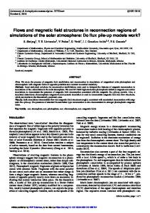
whether the projected curved surface encompasses the center of sphere. According to above information, the method demands a closed curved surface formed by known physical quantities. Four identical spacecrafts of Cluster mission form a tetrahedron in space and the magnetic fields recorded by them will form a closed curved surface. Thus we can calculate and decide whether a null point exists inside the tetrahedron formed by Cluster. Figure 2 shows the projection of tetrahedron to unit sphere[12]. On unit sphere, the recurrent number surround center of sphere (Poincaré index ) is
⎧ ∂B ∂B ∂B ⎪ Bx = x ( x − x0 ) + x ( y − y0 ) + x ( z − z0 ) ∂x r0 ∂y r ∂z r0 ⎪ 0 ⎪ ∂By ∂By ∂By ⎪ ( x − x0 ) + ( y − y0 ) + ( z − z0 ). ⎨ By = ∂x r ∂y r ∂z r ⎪ 0 0 0 ⎪ ⎪ B = ∂Bz ( x − x ) + ∂Bz ( y − y ) + ∂Bz ( z − z ) 0 0 0 ⎪ z ∂x r0 ∂y r ∂z r0 0 ⎩ (2) The equation set consists of 12 unknown variables including 9 variables of δ B matrix and 3 position variables ( x0 , y0 , z0 ). We could transform this equation set
surface S to a unit sphere by Gauss projection
γ : R3 \ {0} → S 2 , v 6
I=
v v
[12]
.
We
need
to
1 1 4 r n S = cos( , )d ∑ sign(Si ) ⋅Si , 4π ∫∫ 4π i =1 S
where Si is the area of spherical triangle formed by projecting three points from tetrahedron to sphere. n is the outer normal of each surface of the tetrahedron after projecting. Obviously, the normal is parallel to r, so sign( Si ) = cos(r , n) = ±1. The method and the geometry properties around null points[2] can be summarized in Table 1. We could use this method to determine whether there is a null point or not, and then reconstruct the local
Figure 2 Table 1 Eigenvalues
into a linear equation set of these variables if the gradient matrix is full rank. Magnetic field and position recorded on each satellite of Cluster will form 3 equations, so the data from the four satellites can be used to exactly form 12 equations. Then we could obtain the position as well as velocity of null point by solving the linear equation set.
2 Analysis of one typical event with 3-D null point in diffusion region We have statistically analyzed the null points inside dif-
Projection from tetrahedron to unit sphere.
γ line (spine)
Σ plane (fan surface) normal v1×v2 v1×v2 u1×u2 u1=v1+ v2; u2 = −i(v1−v2)
Null type and Poincaré index A, index = 1 B, index = −1 v1; v2; v3 As, index = 1 v3 v1; v2; v3 v3 Bs, index = −1 u1×u2 u1 = v1 + v2; u2 = −i(v1−v2) The table does not consider the condition when one or more eigenvalues equals zero. When gradient matrix has the eigenvalue equal to zero, the null will decay into 2D or 1D. The detailed description can be found in the paper of Parnell et al.[2], 1996.
λ1, λ 20 λ1, λ2>0; λ30 λ 1, λ 2 conjugate; λ3