eISSN 2345-0363 Journal of Water Security, 2015, Vol. 1, jws2015002 doi: http://dx.doi.org/10.15544/jws.2015.002
STRUCTURES OF TURBULENT VORTICES AND THEIR INFLUENCE ON FLOW PROPERTIES Alfonsas Rimkus Institute of Water Resources Engineering, Faculty of Water and Land Management, Aleksandras Stulginskis University, Universiteto str. 10, LT-53356 Akademija, Kaunas distr., Lithuania. E-mail:
[email protected] Submitted 22 September 2014; accepted 16 March 2015 Abstract. In spite of the many investigations that have been conducted on turbulent flows, the generation and development of turbulent vortices has not been investigated sufficiently yet. This prevents to understand well the processes involved in the flow. That is unfavorable for the further investigations. The developing vortex structures are interacting, and this needs to be estimated. Physical summing of velocities, formed by all structures, can be unfavorable for investigations, therefore they must be separated; otherwise bias errors can occur. The difficulty for investigations is that the widely employed Particle Image Velocity (PIV) method, when a detailed picture of velocity field picture is necessary, can provide photos covering only a short interval of flow, which can’t include the largest flow structures, i.e. macro whirlpools. Consequently, action of these structures could not be investigated. Therefore, in this study it is tried to obtain the necessary data about the flow structure by analyzing the instantaneous velocity measurements by 3D means, which lasts for several minutes, therefore the existence and interaction of these structures become visible in measurement data. The investigations conducted in this way have been already discussed in the article, published earlier. Mostly the generation and development of bottom vortices was analyzed. In this article, the analysis of these turbulent velocity measurements is continued and the additional data about the structure of turbulent vortices is obtained. Keywords: hydraulic investigations, structure of turbulent vortices, measurement analysis.
Introduction It has been revealed by many previous investigations that there are two main types of turbulent vortices, i.e. the bottom vortices generated near the bottom, where critical velocity gradients are formed, and the macro whirlpools developed along the whole depth of flow. The structure investigated by Vanoni and Nomicos is shown in Fig. 1.
Fig. 1. Distribution of turbulent vortices according to Vanoni and Nomicos (1959)
However, despite abundant literature devoted to investigations of turbulence, the process of the generation and development of these vortices has not been sufficiently explored, despite these vortices having been revealed already for many years (Vanoni, Nomicos, 1959; Klaven, 1966; Grishanin, 1969; Cuthbertson, Ervin, 1999; Nezu, Azuma, 2004). The difficulty is that the
mostly employed PIV method, when a detailed picture of measured velocities is necessary, can provide photos that record only a short interval of the flow, which cannot include even a single macro whirlpool, and their action cannot be investigated. In this study, turbulence was investigated by analyzing instantaneous velocity measurements carried out by 3D means. The measurement in each point takes at least 1 minute, during which all vortices recur many times and can be studied. The investigations discussed in this article are the sequel by the work started earlier. The results obtained have already been published (Rimkus, 2012). The data of measurements, which were carried out in the Hydraulic laboratory of Warsaw Agricultural University in a concrete channel 16 m long and 2.1 m wide with a threecomponent acoustic Doppler velocity meter at a frequency of 25 Hz, were analyzed. Each measurement lasted 6.0 min (9000 measurement steps). The crosssection of the channel and the displacement of measurement verticals are shown in Fig. 2.
Fig. 2. Cross-section of experimental channel and displacement of measurement verticals. The measurements are given in cm. Copyright © 2015 The Authors. Published by Aleksandras Stulginskis University, Riga Technical University. This is an open–access article distributed under the terms of the Creative Commons Attribution–NonCommercial 3.0 (CC BY–NC 3.0) license, which permits unrestricted use, distribution, and reproduction in any medium, provided the original author and source are credited. The material cannot be used for commercial purposes.
14
Journal of Water Security, 2015, Vol. 1, jws2015002
The slope of the channel bed was 0.05%. The water depth H =28.3 cm, and water discharge Q=95.2 l/s. The surface of main channel bed was smooth (Manning roughness coefficient n=0.011 m-1/3s); the floodplains and sloping banks were covered in cement with grains of 0.5 to 1 cm in diameter (n=0.018 m-1/3s). These measurements have already been investigated by the authors. The Reynolds stresses, autocorrelation function, vortex energy spectra were studied (Czernuszenko et al., 2007; Czernuszenko, 2002; Czernuszenko, Rowinski, 2008; Czernuszenko et al., 2007). In the mentioned published earlier article (Rimkus, 2012) the generation and initial growth of bottom vortices and macro whirlpools in the main channel, and the structure of turbulent vortices in the floodplain were discussed. a
The aim of this work was to study the generation and development of structures of turbulent vortices, their interaction and properties. The studied longitudinal and vertical velocities of bottom vortices, formed by their generation at a height of 3 cm from the bottom, shown in Fig. 3. They were found here to be much greater than they became at a height 4 cm, where these vortices were developed further. This means that this quite large energy amount obtained by their generation is distributed in a small volume and is quickly employed for turning of the neighbouring water volume. Afterwards, the vortices develop slowly. They acquire the energy to further their growing from the upper existing flow layers with a higher velocity. b
0.8
0.8
39 transversal 38 37 36 39 vertical 38 37 36
0.6
y/h
0.5
20 y
0.6
5
y 20
39 longitudinal 38 37 36
0.7
15
0.5
y/h
0.7
0.4
10
0.4
10
0.3
0.3
0.2
0.2
5
5
0.1
0.1
0
0 0.2
0.4
0.6
0.8
1
1.2
1.4
1.6
( w − w ) 2 / u*
1.8
2
2.2
(v − v ) 2 / u *
0
0.5
1
1.5
2
2.5
3
3.5
4
(u − u ) 2 / u*
Fig. 3. Turbulence intensity profiles in measurement verticals 39, 38, 37, 36; a – of the longitudinal, b – of the transversal and vertical velocities
The initially formed velocity is not so high in the floodplain, where the bottom is rough, and these eddies are generated at the protuberances of the bottom. Apparently this peculiarity, i.e. the high generation velocity, is characteristic of the flow over the smooth bottom, at which the flow is laminar; therefore the conditions for vortex generation and critical velocity module gradients are different. In this article the development and the peculiarities of the turbulence in main channel are further discussed. Structures of turbulent vortices Structures of turbulent vortices are studied by employing the chronograms of velocity measurements. The difficulty was that the velocities formed by macro whirlpools and by bottom vortices intertwine and therefore macro whirlpools became quite masked. However, in the chronogram, intervals, where the bottom vortices are regular were found and both types of vortices can be studied. Such interval was found in the velocity chronogram, measured at a height 15 cm of 39 vertical between the measurement points 5400 and 6000. This interval had already been used in the previously
mentioned published investigations (Rimkus, 2012). The part of this interval is shown in Fig. 4. The field of turbulent vortices in the main channel was also changed and by the macro whirlpools, formed in the floodplain. Their influence has also already been discussed in mentioned published earlier article. It was necessary to eliminate this influence. The frequency of valley whirlpools is lower than that of those in the main channel; therefore they could be eliminated by the method used for electrical fluctuations described in this published article. The prepared thus chronogram was used for the study of macro whirlpools and bottom vortices in the main channel. A velocity fluctuation graph of macro whirlpools is also created, as this is visible in this interval. This are also shown in Fig. 4. The macro whirlpools divide the flow volume into the intervals with necessary for them length. The bottom vortices and their groups are generated and further developed in their volume. Therefore velocity graph of bottom vortices twist around the graph made by macro whirlpools. The velocities of macro whirlpools in the upper part of flow, i.e. over the center of whirlpools, are positive. In 15
Journal of Water Security, 2015, Vol. 1, jws2015002
the lover part they are negative. So they take part in forming of the vertical velocity distribution in the flow. The velocity graph in Fig.4 show the velocities made by macro whirlpool. They are expressed here as the fluctuations. At the point of contact of two neighbouring whirlpools the longitudinal and vertical velocities of flow are equal to zero. Thus, if the zero axis in Fig. 4 to move to the minimum of fluctuation velocity, where the velocity is equal to zero, then longitudinal velocity graph of macro whirlpool will be received.
The low and equal to zero velocities between the neighbouring macro whirlpools are brought by their turning to the water surface. Here, they grow along the flow, because of formed velocity gradients. However, along the whole water surface they stay less than the velocities existing somewhat deeper in the flow. That was found during many measurements of average longitudinal velocity (for example Nezu et al., 1999). That is the consequence of the existing velocity distribution in the macro whirlpools.
Fig. 4. The longitudinal instantaneous velocities: 1 – longitudinal instantaneous flow velocities measured between measurement points 5750-6000 and 2 – velocity fluctuations formed by macro whirlpools
The macro whirlpools move faster along the flow than the lover part of flow, where the bottom vortices and their structures are developed. This is so because the flow velocity in the central part of macro whirlpools is higher than the average velocity along the flow height. The velocity of macro a whirlpool moving is near to the flow velocity at its turning centre. Macro whirlpools move over the developed structures of bottom vortices and lift them by their back side in the outer zone of flow. Structures of bottom vortices How it is visible in Fig. 4, the thick twists of velocity chronogram, created by the ordinary bottom vortices, are of a very different height. This means that the conditions of their generation are variable. That is caused by the fact that the already generated and growing vortices contain in their turning volume and the points with the critical velocity gradients, in which the new eddies are generated. Consequently, the conditions for the formation of critical velocity gradients become not constant. Generated and growing variable vortices make the generation conditions still more variable. They make the flow appearance chaotic; however structures of the vortices mostly are quite regular. The bottom vortices, developed after their generation, are displaced in the rows of their groups. They were analyzed in the previously mentioned published article. These groups create one kind of their
coherent structures. The best conditions for the forming of bottom vortices and their groups are in the middle between the main parts of neighbouring macro whirlpools; here the largest longitudinal velocity gradients are formed. Therefore the formed groups of vortices become thicker here; consequently the accumulations of these groups are formed. The thick vortex rows of the groups in these accumulations can influence each other, and therefore they operate in unison; consequently they form yet one kind of the large coherent structures of bottom vortices. The distances between the bottom vortices in their groups are not large, therefore only the oldest, existing higher vortex can take the water amounts from upper layer by liquid viscosity and turn them down to the next vortex, which send this volume to the next younger vortex. So the velocity round the group is formed. That is the specific flow formed exactly by the group. The graph of the velocity of the group twist around the velocity graph of macro whirlpools and the velocities of single vortices twist around the curve made by the group. A clearly visible example of the vortex group can be seen in Fig.4 between 5937 and 5949 points. Due to the velocities round the groups, each group of vortices in their accumulations increases the basic velocity in the upper group and decrease it in lower one. Consequently, the velocities in the front part of the accumulation are lower than in back part. Therefore the velocity graph of 16
Journal of Water Security, 2015, Vol. 1, jws2015002
the whole accumulation makes a long twist around the velocity graph of macro whirlpool. This can be searched for in Fig. 4. The graph of all the accumulation velocities is long. The back part of it with higher velocity is clearly visible in the interval 5885 – 5926. The part with the lower velocities appears in the interval 5850 – 5885. The front of accumulation reaches even the peak velocity point of macro whirlpool. The large local twist between 5830 and 5887 points is formed by a large group of bottom vortices that occurred here. This accumulation contains 6 groups of bottom vortices (the intervals 58455863, 5863-5880, 5880-5898, 5898-5907, 5907-5925 and 5918-5928). Thicker vortices and thicker vortex rows in the accumulations are able to create stronger basic velocity for the neighbouring groups; therefore they increase the possibility of create the accumulations further. Weaker eddies create only single groups. As can be seen in Fig.4, before and behind of this large accumulation the more sparsely located single vortex groups are displaced, which are not joined in the accumulations. They are single elements of various vortex constructions. For example, a single group is found between 5938 and 5948 points. A quite large single vortex, not included in the group (incoherent), is visible at the interval 5973-5979. The velocity graphs of these single vortices are twisting around the graph of macro whirlpool, as they do not influence each other to the necessary degree. Such bottom vortices structures are the result of their cooperation with the macro whirlpools, which create the corresponding conditions for their generation. Near the middle of other pair of macro whirlpools, in the interval 5770-5810, another, however quite small accumulation of bottom vortices groups is formed. It was revealed by analyzing the velocity chronograms along their length that the accumulations of vortex groups are mostly quite long. The low velocities formed at the beginning of such structures reach the maximum velocity point of macro whirlpool and even further. Therefore the macro whirlpools are mostly quite masked. The favourable conditions for the generation of the vortex groups in the middle of neighbouring macro whirlpools can mostly make these accumulations quite long. However, the generated and developing vortices and their groups are of variable strength. They are too weak to influent the other ones, and therefore the further creation of their ordinary accumulation is stopped. Thus short accumulations also occur. This happened so that in the favorable and very useful for the study interval, the length of several ones was not masked. It is not quite clear how his occurred. Maybe the slightly cyclic frequency fluctuation of electrical voltage was favourable for it, which caused the periodic fluctuation of water discharge and also the periodic generation of weak bottom vortices. Such cycles were visible in the graph of longitudinal velocity corrections, eliminating the influence of electrical voltage fluctuations, which was placed in the mentioned published article. These characteristic pulsations were found in this favourable interval, and did not occur in the other ones. Maybe the
artificial conditions to receive the short structures of these group accumulations can be created, for example by several small thresholds at the chosen place of the measurement. Maybe the length of these unfavorable structures will be not longer than the distance between the thresholds. The already developed macro whirlpool will not be changed by the thresholds, however becomes not masked. As one can see, the coherent structures of bottom vortices do not consist of accidentally displaced vortices, as it can be imagined (Jimenez, 1998; Kim at al., 1987; Robinson, 1991). Their groups are formed in rows, which are oblique to the direction of flow. The flow formed round the vortex rows makes the velocity direction of flow elements also some what oblique. That is because the directions of flow velocities are found mostly in the ejection and sweep quadrants (Czernuszenko et al., 2007) rather than in the other two, and they are stronger here. The slightly oblique direction of flow is favourable for it. The coherent structures of bottom vortices have already been studied by many investigators. These works were analyzed by Hussain (1983) and Yalin (1992), however the existing structure of their accumulations and their interaction with the macro whirlpools was not established. These peculiarities must still be studied. For the easier study of the coherent structures, they were mostly accepted chaotic, and approximated methods were created. How it is mentioned before, the macro whirlpools lift the developed structures of bottom vortices into the outer zone of flow. Here the gradients of longitudinal velocities are low and the vortices are already not supported. They die gradually because of fluid viscosity, and because of coming into contact with the new bottom vortex structures, which are already growing. The old ones are weaker; therefore their water amounts are absorbed gradually. As a result, they and their kinetic energy are annihilated here. Thus the live of old structures is finished. Such is the so-called bursting process, in which the bottom vortices are generated along the bottom as single eddies, develop further in the flow into the coherent structures and die, lifted by the macro whirlpools to the water surface, coming into contact with anew growing vortices. As one can see, their development and life process continues a long time and is quite complex. It is the result of cooperation of macro whirlpools and bottom vortices. There are and other conceptions of this bursting process presented in the literature and other developments (Hussain, 1983; Yalin, 1992); however these conceptions are not supported by the thorough experimental study and do not account for the interaction of bottom vortex structures and macro whirlpools. Therefore the vortex structures represented by them are not the quite the real ones. The methods created for the estimation of parameters of such objects often need perfection to account for the real existing vortex structures.
17
Journal of Water Security, 2015, Vol. 1, jws2015002
The influence of macro whirlpools to the formation of hydraulic loses The bottom vortices, lifted by the macro whirlpools in the upper part of the flow, still contain quite large turning velocities and kinetic energy. Consequently here and at the contact of old and new vortices are the regions where the intensive suppression of turbulent energy is going on. Stronger macro whirlpools increase the longitudinal velocity gradients at the bottom; consequently the bottom vortices will be generated and developed in this interval more intensively. The speed of lifting and turning of bottom vortices will then also be increased Thus more bottom vortices and more their energy will be brought into the upper part of the flow and into contact with the old and new ones, so the energy losses will be increased. The lower turning of macro whirlpools, decreased for example by the creation of transversal flow across the channel, will decrease the energy losses. It is revealed by the investigations carried out of the river flow that the slight meandering of natural rivers is favourable for the forming of river bed (Grishanin, 1969, 1971, 1974). The spiral flow created in the meanderings brings the macro whirlpools out from the bed and they do not have enough time to grow fully, so they become weaker, consequently the energy loses of this art decrease. The energy losses in the meandering rivers increase only when they meander sufficiently intensively, therefore much energy is employed for turning of the spiral vortices generated by meanderings. Slight meandering of rivers increases their flow velocity and the transport ability of bottom sediments. However, the suspended sediments become less transportable, as the weaker macro whirlpools cannot lift the sediments to the water surface as intensively as the stronger ones do. The reason for these river flow peculiarities becomes clear through analyzing the processes of creation and development of bottom vortices. It is interesting to estimate this kind of hydraulic losses. It is necessary for this to establish the energy of these lifted vortices. Its amount depends on the lifting velocity, formed by macro whirlpools. However, it is difficult to estimate them, as the vertical velocities of whirlpools intertwine with the velocities of bottom vortices even in the favorable interval, where the longitudinal velocities of macro whirlpools are visible, thus it was impossible to separate them. Therefore quite precise calculations of lifted energy cannot be made. However, they can be carried out by accepting suppositions that seem acceptable. The lifting velocities can be estimated approximately from their proportion to longitudinal turning velocities, which can be taken from the velocity graph in Fig. 4. The width of the turning flow element with the vertical turning velocity, as it can be seen in Fig. 1, is about 2 times larger than the width of the turning flow with the horizontal velocities above the center of the whirlpool, which is equal to nearly 2.0 cm/sec. Thus the necessary vertical velocity is about v1=1.0 cm/sec. The kinetic energy of vortices brought to the lifting part of the macro whirlpool can be estimated from horizontal and vertical velocity pulsation
chronograms, measured at a height 11 cm. The hydraulic losses are commonly measured in cm, and the kinetic energy of lifted vortices must be expressed as the height of the water column, i.e. as follows: E=
k 9000
9000
∑ j =1
u 2j + v 2j 2g
,
(1)
where u and v – the measured longitudinal and vertical fluctuation velocity in the flow; j – measurement point number. The height of turbulent energy according to formula (1) is received E=0.019 cm. The amount of lifted energy El can be estimated as follows: El = Eb1v1 ,
(2)
where b1=1.1H – the bright of the lifting section of macro whirlpool; H=28.3 cm – water depth in the channel, v1 = 1.0 cm/sec – the vertical velocity in this section. The macro whirlpool takes the bottom vortices with a new turbulent energy moving along the bottom vortices with higher velocity than the average one of the flow. Their velocity together with the flow is near to the flow velocity at the centre of whirlpool. According to Fig. 1, this height is equal to 0.42 H. Then, according to Fig. 3a, the flow velocity at this height is equal to 39.3 cm/sec. Velocity measurements are performed only to a height equal to 21 cm. For estimation of the average flow velocity, it was assumed that the velocity till the water level is the same as at a height equal to 21 cm. The average was found to be equal to 36.8 cm/sec. Thus the velocity of macro whirlpool along the volume with bottom vertices is vm=39.3-36.8=2.5 cm/sec. Then the amount of new energy found by the moving whirlpool during 1 sec will be as follows: E f = EHvm ,
(3)
The relation between the lifted and new received energy amounts according to formulas (2) and (3) is: k=El/Ef= b1v1/Hvm=1.1Hv1/Hvm=1.1 x 1.0/2.5=0.44. This relation shows what part of received in the flow turbulence takes the lifted and turned to hydraulic loses energy. The energy height of vortices lifted during 1 sec is: El=kE=0.44 x0.019=0.0084. The way length L flowed by water flow during 1 sec is equal to the average flow velocity, i.e. L = 36.8 cm. Thus the additional slope of the flow caused by energy lifting is: il=El/L=0.0084/36.8=0.00022. The slope of the experimental channel was equal to 18
Journal of Water Security, 2015, Vol. 1, jws2015002
0.00050. Thus the additional hydraulic losses caused by lifting of the bottom vortices into the outer zone of flow by macro whirlpools, according to these approximate calculations, can reach almost a half of common losses, i.e. they are quite considerable. Therefore a slight meandering of the riverbed can decrease this part of hydraulic losses sufficiently for its permeability to increase. The main part of hydraulic losses is caused by the interaction of neighbouring bottom vortices and by viscosity of liquid in all the bottom vortices and in macro whirlpools. Characteristics of macro whirlpools The analysis of the instantaneous velocity measurements showed the process of the formation and development of bottom vortices. Macro whirlpools, however, were already formed in the measurement section and the process of their generation and development could not be observed. Direct investigations of their development have not been carried out yet. However, there are several publications in which quite large vortices with dimensions that are scaled with the flow depth are revealed (Tamburinno, Gulliver, 1999; Klaven, 1966). However, their development was not studied in these works, as the length of flume was too short. These vortices are developed from the vortices generated near the bottom. There are shown such growing yet large neighbouring vortices with a distance between them equal to about 3-4 water depths. The oldest of them is greater than others, and already reach the zone with higher longitudinal velocity. Therefore they move along the flow more quickly, and the distances between the vortices increase. Thus these vortices grow and form eventually the real macro whirlpools with the necessary for them distances. They are stable further, as the energy lost due to the fluid viscosity is restored by velocity gradients. However, the generated eddies, future macro whirlpools, develop not so how the future hairpin vortices. The ends of their axis do not bend to the bottom; they grow in to the length. It is not yet clear how it occurs. Maybe their generation conditions are different. Displacement of macro whirlpools along the flow had already started being studied in the mentioned published article. In order to detect all macro whirlpools by computer, the actually existing whirlpools were compared with a standard form whirlpool. For this comparison, a diagram of standard whirlpool was moved along the velocity chronogram until the point where the standard whirlpool was similar to the one being searched for. For this comparison a correlation function was calculated as:
Fj =
1
λ
∑u λ
s tan d j
− u j +i ,
(4)
i =1
where λ – the length of macro whirlpool in measurement time steps (for main channel λ = 100);
u is tan d – longitudinal velocity at the current measurement point of the standard whirlpool; uj+i – the longitudinal velocity of the supposed whirlpool at the measurement
point; j+i, i – the number of the chronogram point, where the searched for macro whirlpool is supposed to begin. The calculated so distances between the macro whirlpools were equal to about 100 measurement steps in the chronograms. However, several of them were not detected because of intensive masking and their number was decreased. It was desirable to estimate them more exactly. The more convenient computer procedure was prepared for these calculations. For each tested length of the macro whirlpool a row of them along the whole chronogram was prepared, as their length is constant. The graph of whirlpool velocities for the forming of this row was taken from Fig. 4. For the estimation of really existing displacement of macro whirlpools, the right their length and begin of their row were searched for. First of all, begin of the first whirlpool in the row was estimated. For this, the point number of this begin was changed by one measurements step, and the average correlation function for all macro whirlpools was calculated. The minimum of the function was searched for. The found its meaning was fixed. That was the inner cycle of procedure. Further, the length of macro whirlpool was changed by the selected step, and begin of the row was estimated again. Naturally this new begin was slightly different. Thus the length of whirlpool with the minimum of correlation function was searched for. So the real length of the macro whirlpool was estimated. The peaks of many macro whirlpools were masked; therefore the computer instead of them had found the peaks made by vortex accumulations, which have the same frequency as macro whirlpools. Therefore the estimated begins of the row were somewhat dispersed. Consequently the calculations became not quite precise and the estimated lengths at all measurement heights were slightly different. Most of them had a length between 99 and 100. To decrease the scattering of calculated length meanings the search interval was narrowed to 99 – 100. Then the average calculated length of macro whirlpools received 99.3 measurement steps. Probably the error of estimated so length was not larger than 0.1. It seems not large, as begin of macro whirlpools can be displaced then no more than trough 5 measurement points. Most exact these calculations was possible to do in the 39th vertical at the height equal to 15 cm, where an interval with regular bottom vortices was found. At this interval the displacement of macro whirlpools was estimated quite correctly. It was interesting to see the macro whirlpools and bottom vortices in the interval, where the whirlpools are very much masked. This is shown in Fig. 5. Near the middles between the macro whirlpools, the ends of quite long accumulations of bottom vortices are placed (intervals 4860-4920 and 4945-5025). Their forepart with low velocities reaches the maximum points of macro whirlpools; consequently the whirlpools are masked and become unremarkable in the chronograms. In the forepart parts of macro whirlpools, where the velocity gradients are low, the single vortices and single their groups are displaced (intervals 4830-4866 and 50205055). Their graph is twisting around a graph of macro 19
Journal of Water Security, 2015, Vol. 1, jws2015002
whirlpool. This interval with single vortices near the point 4950 is less visible as it is masked by the accumulation of bottom vortices. So a displacement sight of bottom vortices and macro whirlpools in the intervals was demonstrated, where the macro whirlpools are masked. Such analysis of vortex displacement became possible only when the macro whirlpools had already been searched for and
became visible; otherwise the masked macro whirlpools could not be seen. For the previously discussed investigations the measurements in the 39th vertical were employed, where the favourable interval was found. The study of macro whirlpools was also carried out in 38-32 verticals. As was estimated before, here they had the same length equal to 99.3 steps. This means that these whirlpools continue across the all bright of the main channel.
Fig. 5. Example of displacement of macro whirlpools and bottom vortices in the region of measurement chronogram where the macro whirlpools are masked
In these verticals it was proved to study also the form of hairpin-like bottom vortices. However, no results were received, as the vertical and transversal measured velocities were very much distorted by the spiral longitudinal vortices, going from the top of the channel slope. They are formed by the transversal flow moving across the main channel, which is caused by a not quite symmetric inflow of water into the model. Unfavourable for investigations physical summing of velocities of macro whirlpools and structures of bottom vortices The previously discussed distribution in the chronograms of velocities formed by macro whirlpools and by accumulations of bottom vortex groups is not favourable for the investigations of the macro whirlpools as they were masked. Such a velocity distribution of macro whirlpools and accumulations makes the chronogram unfavorable for some other investigations also. The velocities of macro whirlpools over their centre are large and positive, while the velocities of accumulations are much less here and even negative. Such velocity differences make their sum in the chronogram very low. The sum becomes even lower than the velocity, formed by the structures of bottom vortices, which can be calculated as the difference between the chronogram velocities and velocities of the already estimated macro whirlpools. Thus the physical sum of velocities, despite it express the really formed summary velocity, which
gradients define the energy loses, it gets formal, and the real velocities of different vortices get masked. Therefore the measured chronograms become unsuitable for direct employment; for example, for immediate calculation of the kinetic energy of the flow. For this the velocities formed by macro whirlpools and by bottom vortices must be separated. These kinds of distortions do not exist by summing all kinds of single bottom vortices and their structures, as the cycles of single vortices are several times shorter than the cycles of their groups, and cycles of single groups are much shorter than the cycles of their accumulations. However, the measured physical sum of velocities made by single bottom vortices, with velocities made by their groups and accumulations, also needs to be separated for their investigations. Their properties are quite various; therefore the interest in studying them individually arose. The energy of flow also cannot be calculated immediately, as the energy depends on the square of the velocity, thus the square of the velocity sum is not equal to the sum of the separate squares. For the right investigations, the velocities formed by different constructions of turbulent vortices must be separated, and their hydraulic characteristics must be calculated individually, otherwise the received results get formal.. It is characteristic that this unfavorable summing of the velocities formed by macro whirlpools and by accumulations of bottom vortex groups had much less 20
Journal of Water Security, 2015, Vol. 1, jws2015002
influence in the valley flow, where the bottom is rough. The high roughness caused the generation of stronger and rarer bottom vortices, for which the increase of velocity gradients, made by the vertical macro whirlpools, was often not sufficient to create the accumulations of their groups. Consequently they stayed single in many intervals (Rimkus, 2012). As one can see, the unfavorable summing is more characteristic of low bottom roughness, when the accumulations of bottom vortex groups are very long. This inconvenient phenomenon can distort and the results of PIV measurements. For example, in the graph of Vanoni (1959) (Fig.1) the elliptic trajectories of macro whirlpool are very asymmetric; however, the received before velocity graph (Fig. 4), revealed in the conditions without the masking of macro whirlpools, is not very asymmetric. Perhaps the PIV measurements of Vanoni were performed in the flood with a flat bottom; therefore the whirlpools were distorted by this unfavorable velocity summing. The accumulations of vortex groups are formed in the front part of macro whirlpools and change here the direction of the visible velocity vector; consequently the sight of macro whirlpool get asymmetric. Maybe in such cases the parallel, control measurements with a rough bottom would be desirable. It would be useful to do it and for this model which measurements, were used in this work. Then maybe the unmasked macro whirlpools would be received faster. Maybe in the rivers and other natural streams, where the roughness is not quite low, this unfavorable phenomenon will be more seldom or not occur. The previously analyzed unfavorable physical summing of turbulent velocities created by the different kinds and structures of vortices was mostly not taken in account. Consequently, the numerical meanings of results of investigations and calculations, employing the measured velocities immediately, became inexact. Maybe this did not cause the discrepant conclusions, however despite this, the applicable calculation and investigation methods need to be perfected, then their results will be better. Separation of vortex velocity graphs, formed by different elements of their structures This separation can be started from the elimination of macro whirlpools. For this, the graphs shown in Fig. 4 can be used. The difference between the velocities in the measurement chronogram and the velocities of macro whirlpools gives the velocity sum of all kinds of bottom vortices. This operation could be carried out in this work in the existing favourable interval. However, such intervals can occur only accidentally and seldom. Therefore it is necessary to have a method for estimating macro whirlpool velocity immediately from the measurement data. For the separation of macro whirlpools it is necessary to estimate their length and the amplitudes and velocity displacement. Their length can be estimated by the previously discussed method. However, a convenient
method for estimating velocities formed by macro whirlpools has not been created. It can be investigated only by the very labor-consuming PIV method. Therefore it is desirable to have an approximate method, which employs the chronograms of performed velocity measurements; even if the macro whirlpools are masked there. The main role in the formation of velocity chronogram play the macro whirlpools, as the velocity graphs, made by the structures of bottom vortices, twist around the graph of macro whirlpools. Therefore the amplitude of macro whirlpools is proportional to the visible bright of chronogram belt. As can be seen in Fig. 4, there are not many velocity graph points higher or lower than of the extreme velocities of macro whirlpools. With the aim of detecting the improper points, the measured velocities were displaced in the row according to their height, i.e. the probability graph was created. It was noticed from this that the maximum velocity of macro whirlpool is equal to the velocity of 13% of probability, and its minimum corresponds to 83%. Perhaps in the other investigations these meanings will not be far from those estimated here, and the calculation will be sufficiently correct. Analogical methods for separation of macro whirlpools can also be used for vertical turbulent vortices. However, their study is more difficult than for longitudinal ones. That is because they are quite masked even in the found favourable for longitudinal vortices interval. For the creation of the necessary methods the connection between the vertical and longitudinal velocities can help. The maximal and minimal vertical velocity points correspond to the points of longitudinal velocities equal to zero, and the zero points of vertical velocities are at the extreme velocity points of longitudinal ones. However, as said before, the possibility of studying the macro whirlpools was found only in the favorable interval. Therefore mostly the sight of macro whirlpool velocities can simply be accepted only by PIV measurements. Maybe it will be possible to assume, that the received once sight will be similar and in flow with other parameters, then it will become typical. Such approximate sight revealed by Vanoni (1959) is presented in Fig. 1. However, it must be much more detailed. The velocities estimated as the difference between the measured and the formed by macro whirlpools ones consist of velocities made by vortices themselves, of velocities formed by their groups and also by the accumulations of these groups. The graph of the vortex velocities twists around the graph of groups and accumulations. These twists are employed for their separation. The beginning and end of neighbouring vortices at the upper part of macro whirlpool are placed at the point of minimum longitudinal velocity. The average velocity along each vortex is equal to the velocity formed by the groups or their accumulations at the middle point of the length of each vortex. So the velocity curve formed by groups and accumulations was calculated. The velocity of single vortices is equal to the difference between common velocity and the calculated velocity of 21
Journal of Water Security, 2015, Vol. 1, jws2015002
groups. For calculation of this difference the velocities of the groups and accumulations at each measurement point are necessary. They were estimated by interpolation between the calculated ones in rare points. For this, the parabola of the 4th power was used. The calculated so both velocity graphs are shown in Fig. 6. As can be seen, the velocity graph of accumulations contains the twits formed by the single velocity groups. For their separation the same method described before was employed. The separated graphs of single groups and of accumulations are shown in Fig. 7. This separation process was possible, as the velocity graph of macro whirlpool was received in the found favourable interval. This occurred as the group accumulations became short here. That was accidental case. However, maybe it is possible to create such
favourable intervals artificially, for example by forming on the bottom of intervals with not high thresholds rows and glass strips. Maybe then accumulations will be formed not longer than the distances between these rows, and they will not be able to mask the macro whirlpools. The already formed macro whirlpools will not be changed by these thresholds. The other vortices will be investigated in the intervals without these means. It seems that in the case of stable electrical voltage, the intervals of necessary length with the short structures of accumulations of vortex groups would be absent, and the favourable for investigations interval would not be received. Thus the artificial method for this purpose will be urgent.
Fig. 6. Longitudinal velocities of separated structures of bottom vortices: 1 - velocities formed by vortex groups and accumulations of the groups, 2 – velocities formed by bottom vortices themselves
Fig. 7. Longitudinal velocities of separated structures: 1 - velocities formed by accumulations of the vortex groups, 2 – velocities formed by single vortex groups
Employing the graphs placed in Fig. 6 and Fig. 7, the energy level of the separated turbulence structures was calculated as follows:
1 E= 250
6000
∑ j =5750
v j2 u* 2
,
(5)
22
Journal of Water Security, 2015, Vol. 1, jws2015002
u* = gRi = 2.29 cm/sec
where vj is a velocity of the formed by analyzed structure of bottom vortices; u* – shear velocity. Here the energy level is expressed as the relation with the shear velocity, which is characteristic for analyzed flow. The following meanings of energy level, contained by all structures of vortices, are received: 1) Fluctuations made by macro whirlpools 0.76 2) Single bottom vortices 0.46 3) Single groups of bottom vortices 0.29 4) Accumulations of vortex groups 0.39 5) Sum of velocities, formed by all kinds structures of bottom vortices 1.90 6) Energy calculated according to the measurement velocities 1.34 As one can see, the amount of kinetic energy, i.e. the turning intensity of vortex groups and their accumulations is quite high. Their sum is even higher than the intensity of the vortices themselves. This means that by developing vortex structures, the turning velocity round the vortex groups is growing quite intensively. In this table the energy height of turbulent vortices calculated according to not separated summary graphs are also given. It is lower than the sum of energy calculated for all separated kinds. The energy estimated according to the measurement data is 1.90/1.34=1.42 times lower than the sum of the energy of all separated ones. This confirms that before to analyzing the influence of all kinds of bottom vortex structures, they need to be separated. From the measurement chronograms the frequencies of velocity fluctuations made by all ascertained constructions of turbulent vortices can be estimated. The macro whirlpools have the largest cycle and the lowest frequency. Their frequency is: f:=v/L,
(6)
where v=36.8 cm/sec – the average flow velocity; L – the length of whirlpool in cm; L=I*N; N=99.3 – the length of whirlpool in measurement steps; I – the distance between measurement points in cm; l=v/n; n=25 – the frequency of measurements. Then f=v/(v/n)*N=n/N=25/99.3=0.252 1/sec. The cycle of single bottom vortices, as can be seen in the chronogram, is equal to 2-4 steps, and the cycle of their groups reaches 5-15 steps, i.e. their frequencies are 6-12 and 16-45 1/sec. The intermediate frequencies between macro whirlpools and single vortices and their groups are absent, as there are no intermediate vortices. However, the calculation by widely employed method for energy spectra gives and the intermediate frequencies (Chernushenko et al., 2007. That is caused by the fact that the macro whirlpools are much masked and their frequency cannot be fixed always and the dispersed between them velocity picks of accumulations make fictive frequencies, as the distances between their neighbouring picks are changing. However, of course
they show the non-existen frequencies. Their frequency is constant and is equal to the frequency of macro whirlpools. By employing this method, it is not taking into account the original peculiarity of the existing vortex structure. This method can give the right results only for the single bottom vortices and for the single their groups, the frequency of which is changing. It is an example of cases when the immediate employing of measurement date gives unreal results. By calculating the length of macro whirlpools according to the previously described method, the fictive much shorter than really existing length equal to 99.3 measurement steps were also accepted. However, they were absent in the favourable interval, where the macro whirlpools were not masked. It also showed the influence of unfavorable summing. The separation process described here was possible as in the velocity graph of measurements a favourable interval was found. This occurred as the accumulations of vortex groups were short here. That was an accidental case. Maybe it is possible, as it was mentioned, to create such favourable intervals artificially by applying in the bottom intervals of necessary length of not high thresholds with glass between them. The distances between them and their height must by chosen experimentally so that the accumulations would be short enough and the macro groups would not be masked The already formed macro whirlpools will not be hanged by the thresholds, the other vortices can be measured without them. Such means would give the possibility of receiving the trajectories of fluid particles in macro whirlpools. Conclusions By generation of the bottom vortices they occur in the rows, so their groups are formed. These groups are their main kind of coherent structures. In the middle between adjacent two macro whirlpools, the gradients of longitudinal velocities are increased; therefore the groups of bottom vortices become here thicker. Consequently they join in the accumulations and make their second kind of coherent structures. The macro whirlpools develop in the initial part of experimental channels from the strongest growing bottom vortices. At the necessary for them distance from the beginning of the channel, they are fully developed. The macro whirlpools flow faster than the layer with the bottom vortices, therefore the back part of the whirlpools lift the already formed vortex structures in the flow upper part. Here they die because of fluid viscosity and due to their contact with anew developing vortex structures. The old vortices are absorbed and their kinetic energy is annihilated, so here a considerable part of hydraulic losses is formed. Their amount grows with the intensity of macro whirlpools, therefore in slightly meandering rivers, where the intensity of macro whirlpools is decreased by the longitudinal spiral vortices formed here, the hydraulic losses are decreased, and the flow velocity is slightly higher. 23
Journal of Water Security, 2015, Vol. 1, jws2015002
The velocity graph of the accumulations of vortex groups make a long twist around the graph of macro whirlpool. Therefore they can be remarked. However, the velocities formed in intervals of accumulations and macro whirlpools are periodically of opposite sign in the same points. Therefore their natural sum in the chronogram gets very low here. Consequently measured chronograms cannot be employed for immediate investigations. Because of such unfavorable physical summing of vortex velocities, the macro whirlpools become quite masked, and they cannot be investigated. In the employed for the study measurements a favourable interval was found, where the length of accumulations was short, and the macro whirlpools were investigated there. However, such cases happen seldom. Maybe the short accumulations can be created artificially, then the macro whirlpools would become unmasked and their study would be possible. The analysis discussed in the article showed that the physical summing in the measurement chronograms of all other kinds of formed in the flow vortex velocities is also unfavorable for investigations . Therefore the components of all different vortex velocities must be separated. The necessary methods are discussed in the article. More attention must become the investigations of macro whirlpools. It is characteristic that this unfavorable phenomenon of velocity summing was not so strong in the valley flow, where the bottom is rough. It results in the bottom vortices and their groups being much stronger and rarer, therefore the additional increase of velocity gradients made by macro whirlpools was not always sufficient to create their accumulations. Thus only the single groups remained, and the unfavorable summing was avoided in many chronogram intervals. It seems that this phenomenon is more available in the flat bottom flows. In such cases a control study with the rough bottom would be useful. Maybe the artificial means for the creation of favourable intervals is possible.Many of the earlier created methods for vortex analysis are needed for their perfection. Acknowledgments I am particularly indebted to Prof. W. Czernuszenko for making available his most recent data on the measurement of turbulence in the water laboratory in Warsaw, as well as for useful discussions. References Cuthbertson, A. J. S.; Ervin, D. A. 1999. The interaction between turbulent vortices and fine sediment particles – a possible reason for enhanced settling characteristics? Proceedings of 28th IAHR Congress. Graz, Austria. CDROM.
Czernuszenko, W. 2002. Turbulent shear stresses and prime velocity distribution in compound channels, Archive of Hydro-Engineering and Environmental Mechanics, 49 (3), 31–45. Czernuszenko, W.; Koziol, A.; Rowinski, P. 2007. Measurements of 3D turbulent structure in compound channel. Archive of Hydro-Engineering and Environmental Mechanics, 54 (1), 55–73. Czernuszenko, W.; Rowinski, P. 2008. Reynolds stresses in a compound open channel – flume experiments. Proceedings of the International Conference on Fluvial Hydraulics, River Flow 2008, 3-5 September 2008, Turkey. 289–297. Grishanin, K. V. 1969. Dynamics of river flow. Leningrad: Gidrometeorologicheskoe izdatelstvo (in Russian). Grishanin, K. V. 1971. Stability of river channels. Meteorology and Hydrology, 10, 69–75. Grishanin, K.V. 1974. Stability of channels in rivers and canals. Leningrad: Hydrometeoizdat. Hussain, A. K. M. F. 1983. Coherent structures-reality and myth. Physics of Fluids, 26(10), 2816–2850. http://dx.doi.org/10.1063/1.864048 Jiménez, J. 1998. The largest scales of turbulent wall flows. Center for Turbulence Research. Annual Research Briefs, 137–153. https://web.stanford.edu/group/ctr/ResBriefs98/jimenez.pdf Kim, J.; Moin, P. S.; Moser, R. D. 1987. Turbulence statistics in fully developed channel flow at low Reynolds number. Journal of Fluid Mechanics, 177, 133–166. http://dx.doi.org/10.1017/S0022112087000892 Klaven, A. B. 1966. Investigation on the structure of turbulent flow. Trudy Gosudarstvennovo Gidrologicheskovo instituta. 136, 65–76 (in Russian). Nezu, I.; Azuma, R. 2004. Turbulence Characteristics and Interaction between Particles and Fluid in Particle-Laden Open Channel Flows. Journal of Hydraulic Engineering, 130(10), 988–1001. http://dx.doi.org/10.1061/(ASCE)07339429(2004)130:10(988) Nezu, I.; Onitsuka, K.; Sagara, A.; Iketani, K. 1999. Secondary currents and bed shear stress in compound open-cannel flows with shallow flood plain. Proceedings of the 28 IAHR Word Congress. Graz, Austria. Rimkus, A. 2012. Structure of turbulent vortices in a compound channel. Archives of Hydro-Engineering and Environmental Mechanics, 59(3-4), 113–135. http://dx.doi.org/10.2478/heem-2013-0003 Robinson, K. 1991. Coherent motions in the turbulent boundary layer. Annual Review of Fluid Mechanics, 23, 601–639. http://dx.doi.org/10.1146/annurev.fl.23.010191.003125 Tamburino, A.; Guliver, J. S. 1999. Large flow structures in a turbulent open channel flow. Journal of Hydraulic Research, 37(3), 363–380. http://dx.doi.org/10.1080/00221686.1999.9628253 Vanoni, V. A. A., Nomicos, G. H. 1959. Resistant properties of sediment-laden streams. Journal of the Hydraulics Division, 85(5), 77-107. Yalin, M. S. 1992. River mechanics. Oxford: Pergamon Press.
24