for simplifying proofs and an automatic theorem prover, called FAUST, for proving the simplified subgoals. 1. INTRODUCTION. Although formal verification of ...
Structuring Hardware Proofs: First steps towards Automation in a Higher-Order Environment Klaus Schneider, Ramayya Kumar and Thomas Kropf University of Karlsruhe, Institute of Computer Design and Fault Tolerance, P.O. Box 6 980, 7500 Karlsruhe, Germany Abstract Most proofs of hardware in an higher-order logic environment follow a definite pattern. T
his observation is used to give a methodology for hardware proofs in order to isolate the s ituations where the designer’s creativity is required, and to automate the remaining tedious p roof tasks. The interactive HOL theorem prover has been extended by generalized hardware specific t actics for simplifying proofs and an automatic theorem prover, called FAUST, for proving the simplified subgoals. 1. INTRODUCTION Although formal verification of hardware has been the focus of extensive research in the r ecent past [1-3], it has not yet been embedded within the toolkit of normal circuit designers. The main reasons for this are twofold --- the existing automatic approaches can handle only a limited class of circuits, and the powerful interactive approaches can be driven only by logicians. In this paper we present a method for structuring hardware proofs within an interactive environment, thus isolating the creative and the routine steps so that effective assistance f or the creative steps and an automation of the latter is made possible. Our approach therefore b ridges the gap between such verification techniques and a normal circuit designer. The automatic approaches which are mostly based on variations of propositional logic, concentrate on proving tautologies [4], or verifying the correctness of finite state m
achines [5, 6]. However, when complete systems or data paths are to be verified, their space/time requirements increase tremendously. Furthermore, the incapability of the inherent p ropositional logic to easily express the concepts of hierarchy and modularity limit their use to the verification of small parts of hardware systems. The interactive approaches on the other hand, are mostly based on higher order logic [7, 8 ]. This logic suffers from the basic drawback that it is incomplete and therefore does not lend itself to automation. However, its expressive power is a great asset for the compact specification and verification of generic hardware [9-11]. Higher order logic can be used to naturally specify the input and output signals of the hardware devices as functions of t ime, and recursively specify generalized n-bit regular structures. It also allows the hierarchical and modular verification of systems, which is a primary requirement in tackling complex s ystems. HOL is a widely used proof assistant for interactive hardware verification in a higher-order logic environment [12, 13]. It is based on natural deduction and uses a small number of a xioms and inference rules for deriving theorems. It also allows the use of user- defined procedures or tactics for combining the inference rules and theorems, thus resulting in a mechanization of
small parts of proofs. However, verifying hardware in HOL requires a great deal of k nowledge in mathematical logic and proof techniques [14]. Our experiences in interactive hardware verification with HOL and LAMBDA [15] and a thorough study of reports have shown that there exists a definite structure in hardware proofs, irrespective of the kind of circuit to be verified, when specifications are to be verified against register-transfer level implementations. On closer examination, we have observed that a large portion of this proof process can be automated and the creative parts, which need i nteractions, can be well isolated. This automation can greatly relieve a normal circuit designer from p roving the correctness of tedious but easily provable formulae, such as “∀ f . ∃ l . ( l t ↔ f t ) ∧ P ( l t ) ↔ P ( f t )”. In order to automate large portions of proofs we have used HOL as a platform for implementing an automatic prover called FAUST (First-order Automation using Unification within a Sequent calculus Technique), which is based on a modified form of sequent calculus called restricted sequent calculus (RSEQ). RSEQ lends itself to an efficient implementation and furthermore the resultant proofs are readable and understandable, since it closely reflects the semantics of the various logical connectives. The paper is organized as follows --- in Section 2, we investigate the structure of hardware proofs in a higher order environment. Section 3 describes the theory behind the restricted sequent calculus (RSEQ). Experimental results are reported in section 4 and section 5 concludes the paper. 2. STRUCTURE OF HARDWARE PROOFS In the following we assume formal descriptions of a circuit specification S at an abstraction level i and an implementation I at the next lower level i+1, both given in higher-order logic as described e.g. in [9]. Step 1: Set Goal G
G: I → S
Step 2: Expand the definitions of I and S
G´: I´ → S´ Step 3: Break the goal into subgoals
Gּ1
G2
…
Gn
G*1
G*2
…
G*n
Step 4: Simplify the subgoals
Step 5: Prove subgoals
Step 6: Save goal as theorem
Figure 1. Structure of a hardware proof
Theorem Prover
Given the formal descriptions of the specification S and the implementation I, the goal of hardware verification is to show the behavioural equivalence of the two descriptions, i.e. I ↔ S. If the specification is incomplete, e.g. only certain safety or liveness properties are to be verified, such an equivalence cannot be shown and instead the implication of the s pecification from the implementation has to be proven, i.e. I → S. In many cases it is possible to structure the steps in hardware verification as depicted in Figure 1, where internal lines (step 4) are connections between different modules of the implementation which are not primary inputs or outputs. In the rest of this section, these six steps are elaborated using the parity circuit as an e xample [12]. An informal specification of the synchronous even parity circuit is as f ollows: Initially the output (out) is set to “T” (true). At every n+1th clock, the output is T iff there have been an even number of T’s on the input line - in. Step 1: Define the specification and implementation and set the goal The informal specification is converted to a formal one by choosing functions and abstract datatypes which closely reflect the notions in the informal specification, so that the v alidation of the formal specification is easy to perform. The use of hardware description languages and automatic conversions to formal specifications allow the use of usual specification t echniques [16]. A possible formal specification of the informally specified “even parity circuit” is a s follows: ∀ in, out. PARITY_SPEC(in, out) := ∀ t . ((out 0 ↔ T) ∧ (out (suc t) ↔ EVEN (in,out)) where the predicate EVEN is defined as ∀ in, out. EVEN(in, out) := ∀ t . (in (suc t) ↔ ¬ out t) The predicate EVEN, encodes the informal specification --- at all time instants, EVEN is true, iff “in t+1” is equivalent to the complement of “out t”.
in
l1
M U X
l3
O N E
R E G
l4
M U X
R E G
l2
out
l5
Figure 2. Parity Implementation The implementation on the other hand, can be automatically derived from netlists as a conjunction of predicates, each of which correspond to the specification of some previously verified component. A black-box treatment of the implementation yields universally q uantified input/output lines and existentially quantified internal lines [9]. The formal description of the parity circuit implementation given in Figure 2 is as follows :
∀ in, out . PARITY_IMP(in,out) := ∃ l1, l2, l3, l4, l5. ∀ t . NOT_SPEC (l2 t, l1 t) ∧ MUX_SPEC (in t, l1 t, l2 t, l3 t) ∧ REG_SPEC (out, l2) ∧ ONE_SPEC (l4 t) ∧ REG_SPEC (l4, l5) ∧ MUX_SPEC (l5 t, l3 t, l4 t, out t) The goal to be proved for the parity example is as follows: ∀ in, out. PARITY_IMP(in, out) ↔ PARITY_SPEC(in, out) Step 2: Expand the definitions of I and S Both specification and implementation usually rely on the usage of predefined predicates a nd modules to keep the descriptions hierarchical, modular and understandable. To perform the proof task, these definitions have to be expanded. The complex datatypes are also refined, to allow rewriting, e.g. a natural number is refined to suc n 0, . Minor user interaction is required here, in order to control the granularity of expansions. Table 1 Formal specifications of the library components Component
Definition
NOT_SPEC (in,out) ONE_SPEC (out) MUX_SPEC (sel,in1,in2,out) REG_SPEC (in,out)
∀ in,out. (out ↔ ¬ in) ∀ out. (out ↔ T) ∀ sel, in1, in2, out. (out ↔ ((sel → in1) ∧ (¬sel → in2))) ∀ in, out. (∀ t. ((out 0 ↔ F) ∧ (out (suc t) ↔ in t)))
Applying this step on the parity example using the definition of the predicate EVEN and the components as specified in Table 1, generates the following formula. ∀ in, out . ∃ l1, l 2, l 3, l 4, l 5. ∀ t . (l1 t ↔ ¬ l2 t) ∧ (l3 t ↔ ((in t → l1 t) ∧ (¬ in t → l2 t))) ∧ (∀ t1. (l2 0 ↔ F) ∧ (l2 (suc t1) ↔ out t1)) ∧ (l4 t ↔ T) ∧ (∀ t2. (l5 0 ↔ F) ∧ (l5 (suc t2) ↔ l4 t2)) ∧ (out t ↔ ((l5 t → l3 t) ∧ (¬ l5 t → l4 t))) ↔ ∀ t . ((out 0 ↔ T) ∧ (out (suc t) ↔ (in (suc t) ↔ ¬ out t)) Step 3: Break the goal into subgoals This is the creative step, where the user has to use his knowledge in breaking up the goal into subgoals, apply proof strategies like induction and use the lemmas needed. Many design specific heuristics can be built in and design decisions be incorporated, to aid the user in this
task [17]. However, due to the very nature of the problem, automating this step is impossible in many cases. In the simple parity example this step is superfluous and can be s kipped. Step 4: Simplify the subgoals Having broken up the original goal into subgoals, the subgoals can then be automatically simplified. This step is also called the unwind step and consists of three main operations, which are executed consecutively, namely (i) conversion to a specialized prenex normal form, (ii) elimination of internal lines, and (iii) simplification of formulae which contain “true” and “false”. Prenex normal form is an equivalent form of the original formula, containing quantifiers a t the beginning of the formula [18]. This operation consists of applying certain quantifier rewrite rules on the formulae in the subgoals, so as to generate a prenex normal form, which is a prerequisite for the application of steps (ii) and (iii). A complete list of the rewrite r ules needed for transforming hardware specific formulae is given in [19]. We list only those rules needed for the parity example in this paper. Rule 1: (∀ t. (P ∧ Q)) → (∀ t. P) ∧ ( ∀ t. Q) Rule 2: (∀ t. P) → P if t is not free† in P z Rule 3: (∀ t. P) → (∀ z [P] t †† ) if z is not free in P Repeated application of these rules on the parity example results in the following d escription ∀ in, out . ∃ l1, l 2, l 3, l 4, l 5. ∀ t . (l1 t ↔ ¬ l2 t) ∧ (l3 t ↔ ((in t → l1 t) ∧ (¬ in t → l2 t))) ∧ (l2 0 ↔ F) ∧ (l2 (suc t) ↔ out t) ∧ (l4 t ↔ T) ∧ (l5 0 ↔ F) ∧ (l5 (suc t) ↔ l4 t) ∧ (out t ↔ ((l5 t → l3 t) ∧ (¬ l5 t → l4 t))) ↔ ∀ t . ((out 0 ↔ T) ∧ (out (suc t) ↔ (in (suc t) ↔ ¬ out t)) The elimination of internal lines also comprises the application of some rewrite rules, so that internal lines are eliminated. The two rules that are needed for the parity example a re: Rule 4: ∀ P, Q. (∃ l. ∀ t. (l t ↔ Q t) ∧ P (l t)) → (∀ t. P (Q t)) Rule 5: ∀ P, Q. (∃ l. ∀ t. (l 0 ↔ a) ∧ (l (suc t) ↔ Q t) ∧ P1 t ∧ P2 (l t)) → (∀ t. P1 t ∧ P2 0 ∧ P2 (suc t)) Rule 4 intuitively states, that those internal lines which are outputs of combinational components “Q” can be directly eliminated by replacing them by their definitions. In the example, after minor syntactical changes, i.e. by reducing the scope of existentially q uantified
† ††
A free variable is a variable which is not bound by any quantifier (for details see [ 18]) z [P]t denotes the substitution of all occurences of t in P, by z
variables to their actual appearance, an application of rule 4 on the internal lines l 1, l3 and l4 results in the following formula: ∀ in, out . ∃ l2, l 5. ∀ t . (l2 0 ↔ F) ∧ (l2 (suc t) ↔ out t) ∧ (l5 0 ↔ F) ∧ (l5 (suc t) ↔ T) ∧ (out t ↔ ((l5 t → ((in t → ¬ l2 t) ∧ (¬ in t → l2 t))) ∧ (¬ l5 t → T))) ↔ ∀ t . ((out 0 ↔ T) ∧ (out (suc t) ↔ (in (suc t) ↔ ¬ out t)) Rule 5 analogously leads to the elimination of those internal lines which correspond to the outputs of sequential components. However, since sequential components may be used for storing internal states, complete elimination of the internal lines is not possible in all cases. Applying this rule using l5 as P1 and out as P2 for eliminating l2, yields the following formula: ∀ in, out . ∃ l5. ∀ t . (l5 0 ↔ F) ∧ (l5 (suc t) ↔ T) ∧ (out 0 ↔ ((l5 0 → ((in 0 → ¬ F) ∧ (¬ in 0 → F))) ∧ (¬ l5 0 → T)) ∧ (out (suc t) ↔ ((l5 (suc t) → ((in (suc t) → ¬ out t) ∧ (¬ in (suc t) → out t))) ∧ (¬ l5 (suc t) → T))) ↔ ∀ t . ((out 0 ↔ T) ∧ (out (suc t) ↔ (in (suc t) ↔ ¬ out t)) Rule 4 can now be applied again to eliminate the internal line l5. The constants “T” and “F” appearing in the formulae due to the initializations of the sequential components, can be eliminated by using the usual logical simplification rules, yielding: ∀ in, out . ∀ t . ((out 0 ↔ T) ∧ (out (suc t) ↔ ((in (suc t) → ¬ out t) ∧ (¬ in (suc t) → out t)))) ↔ ∀ t . ((out 0 ↔ T) ∧ (out (suc t) ↔ (in (suc t) ↔ ¬ out t))) Step 5: Automatic proof of the simplified subgoals Having reduced the subgoals into a simple form, an automated theorem prover can then be used to prove each subgoal separately. The next section is essentially devoted to a brief description of such a prover called FAUST. In many cases, FAUST is capable of proving these subgoals without further aid. However, to speed up the proof process and to contain the space and runtime requirements, it may be necessary to guide the proof process by proving some lemmas. An analysis of the subgoals could lead to an automatic suggestion of the l emmas to be proved before the automatic prover is started.
Step 6: Update library for future use The specification and the correctness theorems generated for the design can then be stored within a library and recalled later while designing components which use the currently v erified component. A hierarchy can thus be achieved in future proofs as the specification and the correctness theorems are sufficient and the current component need not be broken down to its implementation anymore. In this section, we have shown that although hardware verification remains to be i nteractive, most of the drudgery can be automated. The extent to which hardware verification has been automated up to now can be compared by referring e.g. to the tutorial paper on HOL [ 12]. 3. THE THEORY BEHIND FAUST Although higher order logic has been used in the last section to specify and verify h ardware, it is apparent, that only few constructs are necessary, which exceed the expressiveness of first order logic. However we have observed that, it is possible to automate proofs of s tatements in this restricted higher order logic, by means of a calculus which grounds on first order techniques. A theorem prover which is capable of proving subgoals according to the proof structure given in section 2, must be able to prove higher-order formulae. Moreover, to gain c onfidence in the resultant proofs, they have to be readable. This motivated us to implement the prover FAUST, based on a modification of the well-known, proof-tree based, sequent calculus SEQ [18,20], called “Restricted Sequent Calculus (RSEQ)”. The modifications were instigated by the need for an efficient implementation of the γ rules (universal/existential quantifier elimination). In the following we briefly present the underlying ideas of RSEQ. A detailed presentation may be found in [19, 22]. The α-, β- and δ- rules in SEQ are deterministic and hence not critical for the construction of the proof tree. On the other hand, the γ-rules are nondeterministic as an arbitrary term may be chosen for substituting a bound variable. When the formula to be proved is large, often γ-rules have to be applied during the early phases of the proof tree construction. However, the “ right” choice of the substitution heavily influences the length and complexity of the further proof. Hence, the concept of a metavariable is introduced so as to postpone the decision for an appropriate substitution term, until enough decision information is available. The process is performed as follows. If one arrives at a point where a γ-rule has to be applied, a search for an appropriate term is not undertaken. Instead, a new metavariable is introduced and the construction of the proof tree proceeds further. When the construction process is ripened t o an extent that a suitable term can be found, then the term is substituted for the metavariable. The set of variables is split up into two disjoint sets of “normal” variables V and metavariables VM. The introduction of the metavariable poses problems during the δ-rule application, as the constant substituted must be new, i.e. it does not occur in any of the nodes of the proof tree constructed so far. Since the terms corresponding to the existing metavariables are still unknown, a restriction is placed on the metavariables, so that the terms to be substituted for the metavariable do not contain the constants introduced by the δ-rules. To this effect a set called the forbidden set (fsm), fsm ⊆ V is defined, for each used metavariable m ∈ VM, containing all those constants introduced by δ-rule applications after the creation of the metavariable m. An alternative approach which uses skolemization instead of restrictions is given in [ 18]. The sequents that appear in RSEQ are called restricted sequents and have the form Γ 5 ∆ || R, where Γ, ∆ ⊆ F (the set of formulae) and R ⊆ VM × 2V. The restriction R of each sequent belonging to RSEQ consists of list of pairs (m, fsm).
The terms for substitution of the metavariables are found via meta-unification. This is a modification of the normal Robinson’s unification algorithm [23] in such a manner, that only metavariables are considered as substitutable sub-terms. However, only those substitutions σ are allowed which satisfy the property : ∀τ ∈ fsm. τ does not occur in σ(m) for all (m,fsm) ∈ R The proof tree construction otherwise basically proceeds in a manner similar to the normal sequent calculus techniques. The introduction of the metavariables and restrictions requires a modified set of γ and δ-rules. For a detailed description of the complete rule-set and the proof tree construction, the reader is referred to [19,22]. FAUST, which is based on RSEQ has been implemented within the HOL theorem proving environment and is written in ML. Our initial idea was to implement FAUST by using the tactics provided within HOL, so that the reliability of the proofs obtained is high. However, this slowed down the speed of automatic proving so drastically, that we felt the need for implementing a stand-alone prover capable of interacting with HOL. This interaction has b een achieved by introducing the proofs completed by FAUST as theorems, using the “mk_thm” (make theorem) function in HOL. Since this puts us on thin ice, FAUST also generates a HOL tactic, which can then be used to validate the automatic proofs automatically within a normal HOL session. 4. EXPERIMENTAL RESULTS FAUST was first tested for its correctness by using the propositional and first-order formulae taken from [24, 25]. The runtimes of some complex formulae are given in Table 2 and were measured on SUN 4/65 using the ML-package included in the usual HOL- system. The problem called Andrew’s challenge (P34 in Table 2) was solved by generating 86 subgoals as compared to 1600 subgoals generated by resolution provers. Additionally, we have observed that specialized HOL tactics can be developed for difficult problems such as Uruquart’s problems, which was then solved in linear time. Table 2 Runtimes of Benchmark-Formulae [25] Formula P12 P21 P25 P26 P28 P34
Time (Seconds) 0.2 0.4 0.4 0.9 0.7 17.6
Having gained confidence about the correctness of our prover we have looked at some combinational circuits which also required a matter of seconds. At present we have p roved the correctness of only small sequential circuits such as parity, serial adder, flipflops, and m
inmax [26]. The parity, serial adder and flipflop examples did not require any interaction and were proved in a few seconds. Since the minmax example needs interactive steps, we can only qualitatively compare it with a normal HOL run. There, each step is interactive, whereas u sing our approach we had to interact with HOL only while proving the correctness of a c omparator module.
5. CONCLUSIONS AND FUTURE WORK In this paper it has been shown that most hardware proofs can be performed by following the sequence of steps given in section 2. The creative steps involved in proving the c orrectness are few in number and most of the other steps can be automated. Furthermore we have elucidated that, although one needs higher order for specifying hardware, it is a restricted form w
hich can be handled by first-order proving techniques. For this purpose, a modified form of sequent calculus has been proposed which allows an efficient implementation. Currently, we are improving the efficiency of our prover further. We are also working on embedding our approach within a commercial design framework [27], so that verification proceeds hand in hand with design. 6 . REFERENCES 1 2 3 4 5 6 7 8 9 10 11 12 13 14
G. Birtwistle, P.A. Subrahmanyam (Eds.): Current Trends in Hardware Verification and Automated Theorem Proving; Springer Verlag, 1988. P. Camurati, P. Prinetto: Formal Verification of Hardware Correctness: Introduction and Survey of Current Research; IEEE Computer, July 1988, pp. 8- 19. V. Stavridou, H. Barringer, D.A. Edwards: Formal Specification and Verification of Hardware: A Comparative Case Study; Proc. 25th Design Automation Conference (DAC 88), 1988, pp. 197-204. E. Cerny, C. Mauras: Tautology Checking Using Cross-Controllability and CrossObservability Relations; Proc. International Conference on Computer- Aided Design (ICCAD 90), 1990, pp. 34-37. O. Coudert, C. Berthet, J.C. Madre: Verification of Synchronous Sequential Machines Based on Symbolic Execution; Proc. Workshop on Automatic Verification Methods for Finite State Systems, Grenoble, June 1989. J.R. Burch, E.M. Clarke, K.L. McMillan, D.L. Dill, L.J. Hwang: Symbolic Model Checking: 10^20 States and Beyond; Proc. 5th Annual Symposium on Logic in C
omputer Science, 1990. A. Camilleri, M. J. C. Gordon, T. Melham: Hardware Verification using Higher-Order Logic; Borrione (Ed.), Proc. IFIP Workshop on "From H.D.L. Descriptions to Guaranteed Correct Circuit Design", Grenoble 1986, North-Holland, pp.43-67. S. Finn, M. Fourman, M. Francis, B. Harris: Formal System Design - Interactive Synthesis based on Computer Assisted Formal Reasoning; Proc. Intl. Workshop on Applied Formal Methods for Correct VLSI Design, Leuven, November 1989. F.K. Hanna, N. Daeche: Specification and Verification of Digital Systems Using HigherOrder Predicate Logic; IEE Proc. Pt. E, Vol. 133, No. 3, September 1986, pp. 242-254. M. J. C. Gordon: Why High-Order Logic is a good Formalism for Specifying and Verifying Hardware; Milne/Subrahmanyam (Eds.), Formal Aspects of VLSI Design, Proc. Edinburgh Workshop on VLSI 1985, North-Holland 1986, pp. 153-178. J. Joyce: More Reasons Why Higher-Order Logic is a Good Formalism for Specifiying and Verifying Hardware; Proc. International Workshop on Formal Methods in VLSI Design, Miami, January 1991. M. Gordon: A Proof Generating System for Higher-Order Logic; VLSI Specification, Verification and Synthesis, Eds. Birwistle G. and Subrahmanyam P.A., Kluwer, 1988. Proceedings of the Third HOL Users Meeting; Aarhus University, October 1990. P. Loewenstein: Experiences Using a Theorem Prover for Hardware Verification; Proc. International Workshop on Formal Methods in VLSI Design, Miami, January 1 991.
15 Abstract Hardware Limited: LAMBDA - Logic and Mathematics behind Design Automation; User and Reference Manuals, Version 3.1, 1990. 16 R. Boulton, M. Gordon, J. Herbert, J. van Tassel: The HOL Verification of ELLA Designs; Proc. International Workshop on Formal Methods in VLSI Design, Miami, January 1991. 17 S. Kalvala, M. Archer, K. Levitt: A Methodology for Integrating Hardware Design and Verification; Proc. International Workshop on Formal Methods in VLSI Design, Miami, January 1991. 18 M. Fitting: First-Order Logic and Automated Theorem Proving; Springer Verlag, 1 990. 19 K. Schneider: Ein Sequenzenkalkül für die Hardware-Verifikation in HOL; Diploma Thesis, Institute of Computer Design and Fault-Tolerance, University of Karlsruhe, 1 991. 20 J.H. Gallier: Logic for Computer Science: Foundations of Automatic Theorem Proving; Harper & Row Computer Science and Technology Series No. 5, Harper & Row Publishers,New York, 1986. 21 L.C. Paulson: Natural Deduction as higher-order Resolution; Journal of Logic Programming, Vol. 3, 1986, pp. 237-258. 22 K. Schneider, R. Kumar, T. Kropf: Automating most parts of hardware proofs in HOL; Proc. Workshop on Computer Aided Verification, Aalborg, July 1991. 23 J.A. Robinson: A Machine-oriented logic based on the resolution principle; Journal of t he ACM, Vol.12, pp.23-41, 1965. 24 D. Kalish, R. Montague: Logic: Techniques of Formal Reasoning; World, Harcourt & Brace, 1964. 25 F.J. Pelletier: Seventy-Five Problems for Testing Automatic Theorem Provers; Journal o f Automated Reasoning, Vol.2, pp.191-216, 1986. 26 L. Claesen: Preface; Proc. Intl. Workshop on Applied Formal Methods for Correct VLSI Design, Leuven, November 1989. 27 Cadence Design Systems Inc.: User Manuals; July 1989.