Student Teachers' Modeling of Acceleration using a Video-Based ...

Student Teachers’ Modeling of Acceleration using a Video-Based Laboratory in Physics Education: A Multimodal Case Study Louis TRUDEL University of Ottawa Ottawa, Ontario, K1N 6N5, Canada Abdeljalil MÉTIOUI Université du Québec à Montréal Montréal, Québec, H2L 2C5, Canada Gilbert ARBEZ University of Ottawa Ottawa, Ontario, K1N 6N5, Canada

ABSTRACT This exploratory study intends to model kinematics learning of a pair of student teachers when exposed to prescribed teaching strategies in a video-based laboratory. Two student teachers were chosen from the Francophone B.Ed. program of the Faculty of Education of a Canadian university. The study method consisted of having the participants interact with a video-based laboratory to complete two activities for learning properties of acceleration in rectilinear motion. Time limits were placed on the learning activities during which the researcher collected detailed multimodal information from the student teachers’ answers to questions, the graphs they produced from experimental data, and the videos taken during the learning sessions. As a result, we describe the learning approach each one followed, the evidence of conceptual change and the difficulties they face in tackling various aspects of the accelerated motion. We then specify advantages and limits of our research and propose recommendations for further study. Keywords: Kinematics, Video-based laboratory; Case study; High school physics; Multimodal learning.

1. INTRODUCTION The modern way to teach physics, as prescribed by high school physics curriculum, requires teachers to take on new roles and modify their concepts about the nature of science and the acquisition of scientific knowledge [1]. Some researchers [2] propose that student teachers experiment for themselves the scientific approach in an environment similar to that in which they will teach. Having student teachers reflect on their own learning process in this type of environment and providing them with educational tools for teaching physical models, aims to favor within the student teachers a better understanding of physical concepts of motion, of ways to plan an experiment to link the results to an initial hypothesis, and of the usefulness of models in planning and executing experiments. Kinematics, defined as the study of the motion of objects without concern with its causes, has been chosen for this research since this topic presents many difficulties to students. There are two main reasons for these difficulties put forward by the researchers: alternative schemas which the pupils already have on the properties of motion and the emphasis put on the mathematical nature of motion properties in the high school physics laboratory. Firstly, the students have, before arriving in

ISSN: 1690-4524

the Physics course, a broad experience with the properties of motion acquired in their interactions with daily events. This experience although useful in daily life may interfere with learning, especially if the teacher does not take them into account [3]. Moreover, students need to understand, not only the complex relations between acceleration and other kinematical concepts such as position, time, velocity, but also link acceleration (value and sign) with specific types of motion, such as uniformly accelerated and decelerated motion [4]. Secondly, during laboratory activities, kinematics is often taught with an emphasis on applying the right formulas to get anticipated results [5]. For instance, a common pedagogical technique consists in bringing students, at the beginning of the study of kinematics, to the laboratory where they measure different properties of motion which they then represent with graphs. Back in class, they analyze their results and perform calculations with the aid of mathematical expressions to get the values of the position, speed and acceleration with respect to time to confirm the graphed experimental data. And yet, it appears that the pupils perform these various operations without a real understanding of what they are doing [6]. To overcome these difficulties, a video-based laboratory (VBL) has been proposed as a cognitive tool to help students develop more insights for the understanding of physics concepts [7]. One major challenge for students is to recognize the connection between acceleration and real life situations. To meet this challenge, VBL encourages teachers to enhance students’ problem solving skills by bringing interesting and complex realworld problems into the classroom and illustrating them realistically [8]. However, presenting the complexity of realworld problems using text can be difficult to understand for learners, who have limited experience and knowledge. The use of interactive video and dynamic graphics helps make understanding this complexity manageable even to average students. Although the video-based laboratory (VBL) holds many promises for science teaching and learning, it involves users in many technical difficulties. First, students would need to understand how to operate the functions and features of the modelling computer software. Some of these features might be hard for students to master in addition to understanding the target concepts [8]. Second, teachers are expected to guide students through these technical difficulties, but teachers may also need assistance to deal with the technical difficulties. Therefore, it would be important to explore how teachers and

SYSTEMICS, CYBERNETICS AND INFORMATICS

VOLUME 14 - NUMBER 3 - YEAR 2016

25

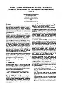
their students interact with videotaping and computer modeling software. Hence, to gain a deeper understanding of the ways learners approach the study of kinematics, it is recommended to involve student teachers in researching this topic for the following reason. Some researchers explain that by acting as students, student teachers have the opportunity to gain pedagogical insights, and by acting as teachers, they have the opportunity to gain content insights [9]. Therefore, by putting student teachers in the role of students, we may gain additional pedagogical insights. This additional benefit helps us achieve our research goals: as learners, the student teachers enable us to ‘model learning of a group of students given specific conditions...in a video based laboratory’ and as future teachers, they help us identify ways of improving student learning. Finally, this study is situated in social constructivism paradigm. We argue that the video-based laboratory can function as intellectual partners with student teachers in order to develop their conceptual understanding of acceleration [10]. Peer interaction present additional experiences that lead student teachers to complete learning tasks more efficiently. Thus, the following research questions were selected for this study: • How do student teachers as learners interact with specific kinematics software within the context of the teachinglearning sequence proposed? What aspects present difficulties for them? And what aspects do they find simple and straightforward? • From an analysis of their learning paths, and their ongoing comments and reflections about it, which teaching strategy/strategies, such as discussions, group work, demonstrations, etc., help student teachers develop conceptual understanding of acceleration? 2. CONCEPTION OF THE LEARNING SEQUENCE In the learning sequence proposed, the kinematic modeling activities have been designed to study the characteristics of the following models: uniformly accelerated motion and uniformly decelerated motion [4]. The experimental set-ups used by the student teachers to study the properties of motion consisted of a rectilinear track of two meters long, one stainless steel ball and three universal supports. Student teachers were asked to assemble each set-up by themselves following the instructions given in the learner’s guide. The ball can be made to roll along the track which can also be inclined (Fig. 1 and 2). As the experiments progressed, student teachers could capture the motion using a digital camera. The digital data were then copied to the computers using a USB connection. These computers contained programs called REGAVI and REGRESSI that are designed to conduct kinematics calculations using digital data of motion [11]. The student teachers were given specific tasks to complete with these programs, such as calculate the ball’s position, speed and acceleration. The researcher acted as a teacher-facilitator by helping the student teachers throughout the lesson, just as a high school teacher would do with his students during a high school physics lesson. To enable student teachers to work together in pairs, we designed an activity guide that was used to manage the student teachers’ lesson. The guide contained two cases for studying various aspects of acceleration concepts [12]. Each case included activities (questions, graphics to be completed, etc.) that guided the student teachers’ modeling process. The modeling process was structured as a POE task (Prediction> Observation> Explanation) [13].

26

SYSTEMICS, CYBERNETICS AND INFORMATICS

The first case of uniformly accelerated motion was presented to the student teachers in the guide as follows. The ball A is released from the top of the incline at rest. The position of the ball (A) after 1 second is preseted using figure 1. As part of the prediction task, the guide asks the student teachers to draw by hand on the figure 1, the positions he expected the ball (A) will be during the seconds following the release. They also had to answer the following questions. What happens to the motion of the ball? Does its motion remain the same all the way? What happens to the speed of the ball?

1 2 meters

Fig. 1. Motion of a ball rolling down an inclined track

The second case involved a uniformly decelerated motion. A ball is pushed up an inclined track. Student teachers were asked to predict its motion in a way similar to the first case. After predicting the motion of the balls for each of the cases, the guide asks student teachers set up and complete the experiments as explained above.

1 Fig. 2 A ball is pushed up an inclined track with an initial speed.

3. METHODS Description of the context of the study The research participants recruited for this study were two male teacher candidates at the university where the study was carried out. As students in the teacher training program, they held a previous bachelor degree in science or an equivalent diploma. They were volunteers and had been selected because of their availability for the scheduled dates of the study which consisted in completing two activities where they studied the properties of motion and discussed with each other the scientific and educational aspects of the process. The activities were held in a single 2.5 hour session scheduled during the session study week. Activities took place in a special laboratory room where four cameras covered most of the area where the future teachers completed the activities and two cameras recorded the student teachers’ interactions with their respective computer. One member of the research team acted as the teacher during the study. His role consisted of introducing the activities to student teachers, of assigning them roles during small group discussions, and completing in a plenary the analysis and

VOLUME 14 - NUMBER 3 - YEAR 2016

ISSN: 1690-4524

synthesis of their results at the end of each activity period. As such, the researcher was present during each activity. The researcher also played the role of lab monitor to help with difficulties that arose in the set-up, the software data collection or analysis obtained by the student teachers. He introduced them to the required computer programs features before student teachers had to use them for data collecting and analysis in each activity. He also led a discussion with student teachers at the end of each activity to summarize their results and discussed the difficulties encountered as well as their suggestions to improve the activities [14]. Data collecting and analysis methods This study implemented a qualitative case study approach for collecting and analyzing the data [15]. The researchers explored in depth the interaction of the two student teachers with computer modeling software program while they were studying the concepts of speed and acceleration. A time limit was placed on the learning activity during which the researcher collected detailed multimodal information using student teachers’ artifacts and videos developped during the learning sessions [16]. Additionally, we set out to use the participants’ artefacts to identify preconceptions that seemed most likely to affect their understanding of speed and acceleration. Specifically, we were trying to ascertain participants’ expectations of the graphical representations of object motion as well as their preconceived ideas about the concept of acceleration as observed in the experiments or from the graphs.

Fig. 3 Sketch drawn by ST1 of his predictions about the successive positions versus time of the ball rolling down an incline in case 1. Indeed, ST1 did not make a distinction between the graph of the position versus time and the graph of the speed versus time (Fig. 4 and 5). Hence, comparing these two graphs, one can conclude readily that their shape looks very similar (Fig. 4 and 5)

Fig. 4 Predicted Cartesian graph of position-time (left) by ST1 for case 1

To study the learning process of student teachers, we analyzed the content of the activity guides student teachers had to fill. Content reported by student teachers in these guides were expressed in different ways: text when answering questions, iconic in sketches of the moving ball, Cartesian graphs when predicting position-time and velocity-time aspects of motion. Qualitative data collected in these various forms of presentation received a categorization analysis [17].

4. PRESENTATION AND ANALYSIS OF RESULTS For clarity, we have classified the responses of student teachers according to the two phases of the POE task where they had to answer questions, namely the prediction and explanation, as well as some details about the experiment process (data collecting and analysis) when appropriate. We will present separately the results about the uniformly accelerated motion (case 1) and uniformly decelerated motion (case 2). Results of case 1: uniformly accelerated motion In the first case of uniformly accelerated motion, when asked what would happen to the ball when released from the top of the inclined track, the first student teacher (coded ST1) answered that the motion won’t be the same as it rolls down (fig. 3).

ISSN: 1690-4524

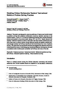
Fig. 5 Predicted Cartesian graph of speed-time by ST1 for case 1 When analyzing data using the computer software REGRESSI, ST1 encountered difficulties matching the formula of a parabola to graphed data of position versus speed. Observations from the video taken by one camera that monitored his interactions with the computer software showed that ST1 did not take into account in his modeling that the initial time shown in the position-time graph was not zero (Fig. 6). However when ST1 compared his predicted graphs of position-time or speed-time (Fig. 4 or 5) with the their respective graphs obtained through REGAVI and REGRESSI software (Fig. 6 or 7), he was quick to recognize that the positions predicted were in agreement with the data collected but that the speeds predicted were not. Hence, ST1 concluded the shape of the curve of the speed versus time is a straight line since the slope of the curve is a constant (Fig. 7).

SYSTEMICS, CYBERNETICS AND INFORMATICS

VOLUME 14 - NUMBER 3 - YEAR 2016

27

x (m)

prediction to his colleague, he drew the graph of position with respect to time as shown in Fig. 9.

0.8 0.7 0.6 0.5 0.4 0.3 0.2 0.1

0.5

1

1.5

2

2.5 t (s)

Fig. 6 Cartesian graph of position-time obtained by ST1 using REGAVI and REGRESSI software for case 1

Fig. 9 case 2

Predicted Cartesian graph of position-time by ST1 for

In predicting the changes in speed, he expressed verbally that the speed would decrease linearly with time while going uphill and that the speed would increase linearly while going downhill. Again, he drew at the same time his predicted speedtime graph (Fig. 10).

v (m/s)

0.8

0.6

0.4

0.2

0.5

1

1.5

2

2.5 t (s)

Fig. 7 Cartesian graph of speed-time (right) obtained by ST1 using REGAVI and REGRESSI software for case 1 Finally, when asked to compare the motion of the ball rolling down an incline with the motion of the ball traveling on a horizontal plane, ST1 stated that the speed of the ball on the horizontal track was constant while the speed of the ball on the inclined track increased linearly. The second student teacher (coded ST2) did not encounter the same difficulties since he predicted correctly the scientific model of motion. Indeed, he predicted that the position of the ball rolling down the incline would be a parabola and that the increase of speed versus time would be linear. So when he compared his predictions with the results of experimentation, he stated that they were in agreement.

Fig. 10 Predicted Cartesian graph of speed-time-time by ST1 for case 2 When questioned by the researcher about the speed of the ball at the summit, he answered that the ball would stay at rest for no more than a second. He added that he learned from the previous case that in both parts of the graph given in his prediction (upward motion and downward motion), the curve of the speed versus time would be a straight line. In the explanation phase, ST1 wrote that the results he obtained via computer were in agreement with his predictions (Fig. 11 and 12). However, he left unexplained the right part of the parabola where the position X does not come back to zero. Neither, did he explained, as ST2 did, that the values of speed are negative in the right part of the graph of the speed versus time obtained by computer (Fig. 12). x (m)

Results of case 2: Uniformly decelerated motion With respect to the second case about uniformly decelerated motion, the first teacher ST1 drew on the guide his prediction about the points occupied by the ball while rolling up the inclined track as shown in Fig. 8.

0.5

0.4

0.3

0.2

0.1

Fig. 8 Sketch drawn by ST1 of his predictions about the successive positions versus time of the ball rolling up an incline in case 2.

0.5

1

1.5

2

2.5

3 t (s)

Fig. 11 Cartesian graph of position-time obtained by ST1 using REGAVI and REGRESSI software for case 2

Justifying his predictions verbally, he stated that the distance travelled decreased more and more during identical time intervals during ascent. He added that in the descent the distance traveled in identical time intervals was growing more and more as the ball went downhill. While he was justifying his

28

SYSTEMICS, CYBERNETICS AND INFORMATICS

VOLUME 14 - NUMBER 3 - YEAR 2016

ISSN: 1690-4524

v (m/s)

ST1 in case 2 which is more complex than the case 1 since case 2 included a deceleration in the rise and acceleration in descent. Aside from the issue of the sign of the acceleration during descent (predicted by ST2 but not ST1), predictions by the two student teachers are both consistent with the results and graphs. How can we explain such a result that appeared in the answers of ST1?

0.6

0.4

0.2

0

-0.2

-0.4 0.5

1

1.5

2

2.5

3 t (s)

Fig. 12 Cartesian graph of speed-time obtained by ST1 using REGAVI and REGRESSI software for case 2 The second student teacher (ST2) provided more detailed predictions. Indeed, although his predicted position-time and speed-time graphs are similar to those of ST1, the second student teacher’s predicted sketch of position over time showed additional information that allows us to conclude that the he understood this type of motion (Fig. 13).

Fig. 13 Sketch drawn by ST2 of his predictions about the successive positions of the ball rolling up an incline for case 2 Indeed, in the Fig. 13, one can see that the student had drawn in the descent, the positions of the ball at the following times of 6, 7, 8 seconds which correspond to positions of the ball at 4, 3, 2 seconds in the ascent respectively, illustrating the perfect symmetry of the ascent and descent. Moreover, in the previous question, he replied (free translation): "The speed curve contains a center of symmetry. In both parts of the path, the slope of the speed is the same. In the ascent and descent phases, the ball has the same behavior (i.e. speed) if we do not take into account the direction". According to us, the point of view expressed by ST2 reveals a sophisticated understanding of this type of motion. 4. DISCUSSION We have seen that the first case of uniformly accelerated motion had uncovered misconceptions by the first student teacher (ST1). First, ST1 did not differentiate between position and speed while drawing his predicted graphs of position-time and speed-time. This confusion between position and speed was first reported by [18]. However, ST1 showed also difficulties in determining the initial and final values of position and speed at the extremities of the time intervals. In the case of ST2, his sophisticated understanding of motion, both conceptually and mathematically, showed in both cases. However, what is surprising in the second case is not that predictions of both student teachers were in agreement with the scientific model [4], but rather the absence of misconceptions of

ISSN: 1690-4524

Indeed, when we compare ST1 answers in case 2 to those he offered in case 1, we are compelled to note that the confusion between the predicted position-time graphs and velocity-time had disappeared. Moreover, the drawing of the predicted position-time graph could not be obtained by making a copy of his curve from the previous case since the curve in case 2 is an inverted parabola. Not only did ST1 know that the position varies according to the time as a parabola but he discusses in his dialogue with his colleague the symmetry of the ascent and descent. In case 2 for speed-time, ST1 predicted the correct behavior not taking into account the reversal of sign, if one compares the prediction graph (Fig.10) with the graph obtained by computer (Fig 12), . How could one explain such progression in ST1’s concept about speed versus time in such a short time? Suppose that ST1 took his responses from his colleague ST2, who demonstrated an accurate knowledge of acceleration and deceleration. However, the video of interactions between the student teachers showed that ST2 had turned over his documents so that his answers were not visible to ST1. We must then conclude that in whole or in part the teaching-learning sequence contributed in some way to ST1’s gain in understanding the speed behaviour. Moreover, apparent in the recorded video, ST1 made gestures to accompany his justification of his predicted position-time and velocity-time graphs in the second case. For example, he indicated by gestures the increase or decrease of speed while illustrating with a finger the instant when the speed was zero at the summit of the trajectory. Thus it appears that his gestures were in agreement with his drawings and graphs of positiontime and speed-time. Comparing other results in the literature about the link between gestures and other modes of communication, it was found that information expressed by gestures may be in contradiction with the information expressed in other forms of communication when students are in a transitional state of understanding. Since in our study demonstrates that ST1’s gestures and predicted graphs were in agreement, he may have already completed his transition toward better understanding of constant deceleration, at least for the functional relationship between position and time as well as speed and time. However, this transition to higher understanding within ST1 may have only been partial. The fact that he did not explained the right part of position-time and speed-time graphs obtained during experimentation for the second case, may indicate that he still has difficulties tackling the issue of initial and final values of positon/speed at the extremities of time intervals. 5. CONCLUSION From our results, it appears that multi-modality learning not only allow to document the traces of conceptual change but also may help to induce it. For example, in learning sequence used in the study, there were many tasks that included different modalities: manipulation to assemble the experimental set-up,

SYSTEMICS, CYBERNETICS AND INFORMATICS

VOLUME 14 - NUMBER 3 - YEAR 2016

29

peer discussion, answering questions in the guide (predictionexplanation) and adjusting data to the simulation curve. Since our results tend to show that conceptual change appears at least for the first student teacher (ST1), these elements may be supporting a better understanding of kinematical concepts. One must not forget the pivotal role of the computer that is not restricted to the ease of data collecting and analysis, but that also is a cognitive tool to help student teachers actively compare their mental representation with various multiple concrete representations [20]. Moreover, the computer can give the user the possibility to review at will and even stop the motion at some critical points, as well as give an idea of the relationship between various quantities (time, position, speed, acceleration) and test quickly and efficiently various hypothesis emitted by student teachers. This case study involving only two teacher students cannot claim the generalization of results or be transferred to the classroom [15]. This research may help to illustrate the opportunities that technology offers to inform us about the process and difficulties of students that conduct investigations in the science laboratory. In this way, we can learn about how to produce better computer-assisted science laboratories for students. Future research should involve multiple case studies both with a larger and more diversified sample of student teachers as well as a larger number of cases in various scientific disciplines. 6. REFERENCES [1] R.E. Anderson, "Reforming science teaching: What research says about inquiry", Journal of Science Teacher Education, vol. 13, no 1, 2002, pp. 1-12. [2] Aiello - Nicosia, M. L. & Sperandeo - Mineo, R. M., “Educational Reconstruction of Physics Content To Be Taught and of Pre-Service Teacher Training: A Case Study”, International Journal of Science Education, 2000, Vol.22(10), 2000, pp.1085-97. [3] R.D. Knight, Five Easy Lessons: Strategies for Successful Physics Teaching. San Francisco: Addison Wesley, 2004. [4] I.A. Halloun, Modeling theory in science education, Boston : Kluwer Academic Publishers, 2004. [5] A.B. Arons, A guide to introductory physics teaching, 2nd ed. Toronto: John Wiley & Sons, 1997. [6] G. De Vecchi, Enseigner l’expérimental en classe: Pour une véritable éducation scientifique, Paris : Hachette, 2006. [7] L.T. Escalada & D.A. Zollman, D.A., “An investigation on the effects of using interactive digital video in a physics classroom on student learning and attitudes”, Journal of Research in Science Teaching, Vol. 34, No. 5, 1997, pp.467-489. [8] L. Trudel & A. Métioui, “Effect of a video-based laboratory on the high school pupils’ understanding of constant speed motion”. International Journal of Advanced Computer Science and Applications, Vol. 3, No. 5, 2012, pp.71-76. [9] J. Bowers & H.M. Doerr. “An Analysis of Prospective Teachers' Dual Roles in Understanding the Mathematics of Change: Eliciting Growth with Technology”. Journal of Mathematics Teacher Education, Vol.4, No.2, 2001p.115-37. [10] D.W. Russell, K.B. Lucas and C.J. McRobbie, “Role of the Microcomputer-Based Laboratory Display in Supporting the Construction of New Understandings in Thermal

30

SYSTEMICS, CYBERNETICS AND INFORMATICS

Physics”, Journal of Research in Science Teaching, vol. 41, no 2, 2004, pp. 165-85. [11] G. Durliat & J.M. Millet, « L’informatisation des dosages phmétriques avec l’interface Orphy et le logiciel Regressi ». EPI, Vol. 64, 1991, pp. 163-172. [12] P. Yuk Ko & F. Marton, F (2004). Variation and the secret of virtuoso. In F. Marton & A.B.M. Tsui (Eds.), Classroom discourse and the space of learning, pp. 43-62, Mahwah (NJ): Lawrence Erlbaum Associates, 2004. [13] R.F. Gunstone & I.J. Mitchell, “Metacognition and conceptual change”, In J. Mintzes, J.H. Wandersee & J.D. Novak (Eds.), Teaching science for understanding: A human constructivist view, pp. 133-163. Toronto: Academic Press, 1998. [14] S. Rodrigues, J. Pearce & M. Livett, M., “Using video analysis or data loggers during practical work in first year physics”. Educational Studies, Vol. 27, No. 1, 2001, pp. 32-43. [15] T. Karsenti & S. Demers, “L’étude de cas”, In T. Kaesenti & L. Savoie.-Zjac (Eds.), La recherche en éducation: Étapes et approches, 3rd ed., pp. 229-252, St-Laurent (Québec): ERPI, 2011. [16] G. Kress, C.Jewitt, J. Ogborn & C.Tsatsarelis, Multimodal teaching and learning: The rhetorics of the science classroom, New York: Continuum, 2001. [17] M.B. Miles, A.M. Huberman & J. Saldaña. (2014). Qualitative data analysis: A methods sourcebook. Washington (DC): SAGE, 2014. [18] D.E. Trowbridge & L.C. McDermott, “Investigation of student understanding of the concept of velocity in one dimension”. American Journal of Physics, Vol. 48, No 12, 1980, pp. 1020-1028. [19] S. Goldin-Meadow, & M.W. Alibadi, “Looking at the hands through time: A microgenetic perspective on learning and instruction”. In N. Granott & J. Parziale (Eds.), Microdevelopment: Transition processes in development and learning, pp. 80-105, New York: Cambridge University Press, 2002. [20] W. Schnotz & A. Preuβ, “Task-dependent construction of mental models as a basis for conceptual change”. In G. Rickheit & C. Habel (Eds.), Mental models in discourse processing and reasoning, pp. 131-167, Toronto: Elsevier Science B.V, 1999.

VOLUME 14 - NUMBER 3 - YEAR 2016

ISSN: 1690-4524