Study of the Approximate Solution of Fuzzy Volterra ...

42567

Kirtiwant P Ghadle and Ahmed Abdullah Hamoud./ Elixir Appl. Math. 98 (2016) 42567-42573 Available online at www.elixirpublishers.com (Elixir International Journal)

Applied Mathematics Elixir Appl. Math. 98 (2016) 42567-42573

Study of the Approximate Solution of Fuzzy Volterra-Fredholm Integral Equations by using (ADM) Kirtiwant P Ghadle and Ahmed Abdullah Hamoud Dr.Babasaheb Ambedkar Marathwada University, Aurangabad, 431004, India. ARTICLE INFO

Ar t icl e hi s to r y: Received: 02August 2016; Received in revised form: 01 September 2016; Accepted: 7 September 2016; K ey w o rd s Ad o mia n De co mp o s it i o n Met ho d , F uzz y Vo lt erra - Fr ed ho l m I n te gra l Eq u at i o n, Ap p r o xi ma te So l ut i o n, S ys te m of Vo l ter r a Fr ed ho l m I n te g r al Equat io n.

AB S T RA C T A n u me ri cal me t ho d fo r so l v i n g fu zz y Vo lt erra -F red ho l m i n te gra l eq ua tio n o f t h e se co nd k i nd wi ll i s i n tro d uced . W e c o n ver t a no nl i near fuz z y Vo l ter r a - Fr ed ho l m i n te gra l eq ua t io n to a no n l in ear s ys te m o f Vo lt err a Fr ed ho l m i nte gr al eq ua t io n i n cr isp ca se . W e u s e Ad o mi a n De co mp o si ti o n Met ho d ( AD M) to fi nd t he ap p ro xi ma te so l u tio n o f t h is s ys t e m a nd he nc e o b tai n a n ap p ro x i ma tio n fo r fu zz y so l ut io n o f t he no n li ne ar fuz z y Vo lt erra Fr ed ho l m i n te gr al eq ua t io n . Al so , so me n u mer i cal e xa mp le s ar e i ncl ud ed to d e mo n str at e t h e va lid it y a nd ap p l ic ab i li t y o f t he p ro p o s ed t ec h ni q ue.

Introduction The topic of fuzzy integral equations which has attracted growing interest for some time, in particular in relation to fuzzy control, has been developed in recent years. Babolian et. al [1] proposed another numerical procedure for solving fuzzy linear Fredholm integral of the second kind using Adomian method. Moreover, Friedman et. al [7] and Seikkala in [2] defined the fuzzy derivative and then some generalizations of that have been investigated in [3, 4]. Consequently, the fuzzy integral which is the same as that of Dubois and Prade in [5]. However, there are several research papers about obtaining the numerical integration of fuzzy-valued functions and solving fuzzy Volterra and Fredholm integral equations [6, 7, 8, 10, 11, 12, 13, 14, 17]. As we know the fuzzy differential and integral equations are one of the important part of the fuzzy analysis theory that play major role in numerical analysis. The concept of fuzzy numbers and arithmetic operations on it was introduced by Bede [3] which was further enriched by Dubois and Prade [17]. Also they [16] was introduced the concept of integration of fuzzy functions. Chang and Zadeh [15] studied on fuzzy mapping and control. Dubois and Prade [16, 17] made a significant contribution by introducing the concept of fuzzy numbers and presented a computational formula for operations on fuzzy numbers. Shao and Zhang [21] chose to define the integral of fuzzy function, using the Lebesgue-type Tele: 00918087270373 E-mail address: [email protected] © 2016 Elixir all rights reserved

© 2016 Elixir All rights reserved.

concept for integration. One of the first applications of fuzzy integration was given by Wu and Ma who investigated the fuzzy Fredholm integral equation of the second kind. Recently, Ghadle and Ahmed [9] solved Volterra-Fredholm integral equations by using Legendre and Chebyshev collocation methods. The properties of Chebyshev or Legendre polynomials are used to reduce the system of Fredholm integral equations to a system of nonlinear algebraic equations, some mathematician have studied solution of fuzzy integral equation by numerical method [2, 21, 22]. Bildik and Inc studied the approximate solution by using modified decomposition method for nonlinear Volterra-Fredholm Integral Equations [11]. Wazwaz studied new algorithm for calculationg adomian polynomials for nonlinear operators [23]. Gohary found an approximate solution for a system of linear fuzzy Fredholm integral equation of the second kind with two variables which exploit hybrid Legendre and blockpulse functions, and Legendre wavelets. In present, we try to employ Adomian decomposition method for solving fuzzy nonlinear Volterra-Fredholm integral equation. The structure of this paper is organized as follows: In Section 2, the basic concepts of fuzzy number and fuzzy set are discussed. In Section 3, we convert a fuzzy nonlinear Volterra-Fredholm integral equation to a nonlinear system of Volterra-Fredholm integral equation of second kind in crisp case and approximate

42568

Kirtiwant P Ghadle and Ahmed Abdullah Hamoud./ Elixir Appl. Math. 98 (2016) 42567-42573

(FVFIE) with ADM. We present and describe the basic formulation of the ADM required for our subsequent development, in Section 4. Finally, in Section 5, we will give report on our numerical findings and demonstrate the accuracy of the proposed scheme by considering numerical examples, and a brief conclusion is given in Section 6. Basic Concepts Fuzzy numbers generalize classical real numbers and we can say that a fuzzy number is a fuzzy subset of the real line which has some additional properties. The concept of fuzzy number is vital for fuzzy analysis, fuzzy differential equations and fuzzy integral equations, and a very useful tool in several applications of fuzzy sets. Basic definition of fuzzy numbers is given in [6, 17]. Definition 2.1. A fuzzy number is a fuzzy set like ω: R → [0, 1] with the following properties: (i) ω is upper semi-continuous function, (ii) ω is fuzzy convex, i.e, 𝜔 (𝜆 𝑥 + (1 − 𝜆)𝑦) ≥ 𝑚𝑖𝑛{𝜔(𝑥), 𝜔(𝑦)} ∀ 𝑥, 𝑦 ∈ 𝑅 , 𝜆 ∈ [0,1], (iii) ω is normal, i. e, ∃ 𝑥 0 ∈ 𝑅 for which 𝜔(𝑥 0 ) = 1, (iv) Sup 𝜔 = {𝑥 ∈ 𝑅| 𝜔(𝑥) > 0} is the support of the ω, and its closure cl(sup ω) is compact.

distance between fuzzy numbers given by 𝑑 ∶ 𝐸 × 𝐸 → 𝑅+ ∪ {0}. 𝑑(𝜔, 𝑣) = sup max{|𝜔(𝛼) − 𝑣(𝛼)| , |𝜔(𝛼) − 𝑣(𝛼)|} 𝛼∈[0,1]

where 𝜔 = (𝜔(𝛼), 𝜔(𝛼)), 𝑣 = (𝑣(α), 𝑣(α)) ⊂ R are utilized in [15]. Then, it is easy to see that d is a metric in E and has the following properties (see [3]): (i) 𝑑(𝜔 + 𝜌, 𝜐 + 𝜌) = 𝑑(𝜔, 𝜐), ∀𝜔, 𝜐, 𝜌 ∈ 𝐸, (ii) 𝑑(𝑘𝜔, 𝑘𝜐) = |𝑘| 𝑑(𝜔, 𝜐), ∀ 𝑘 ∈ 𝑅; 𝜔, 𝜐 ∈ 𝐸, (iii) 𝑑(𝜔 + 𝜐, 𝜌 + 𝑒) ≤ 𝑑(𝜔, 𝜌) + 𝑑(𝜐, 𝑒), ∀ 𝜔, 𝜐, 𝜌, 𝑒 ∈ 𝐸, (iv) (𝑑, 𝐸) is a complete metric space. Definition 2.3 [8]. Let 𝑓 : R → E , be a fuzzy valued function. If for arbitrary fixed t0 ∈ R and 𝜖 ≥ 0, 𝛿 ≥ 0 such that |t − t0| < δ  is said to be continuous. Theorem 2.1 [17]. Let

f ( x) be a fuzzy valued function on

[𝑎, ∞) and it is represented by ( f ( x,  ), f ( x,  )) . For any fixed α ∈ [𝑎, 𝑏] assume

f ( x,  ) and f ( x,  ) are Riemann-

integrable on [𝑎, 𝑏] for every 𝑏 ≥ 𝑎, and assume there are two 𝑏

positive 𝑀(α) and 𝑀(α) such that ∫𝑎 |𝑓(𝑥, 𝛼)| 𝑑𝑥 ≤ 𝑀(𝛼) 𝑏

and ∫𝑎 |𝑓(𝑥, α)| 𝑑𝑥 ≤ 𝑀(α) for every 𝑏 ≥ 𝑎. Then

f ( x)

is

Let E be the set of all fuzzy numbers on R. The α-level set of a fuzzy number ω ∈ E, 0 ≤ α ≤1, denoted by [ω]α, is defined as

improper fuzzy Riemann integrable on [𝑎, ∞) and the improper fuzzy Riemann-integral is a fuzzy number. Furthermore, we have: ∞ ∞ ∞ ∫𝑎 𝑓(𝑥) 𝑑𝑥 = (∫𝑎 𝑓(𝑥, 𝛼) 𝑑𝑥, ∫𝑎 𝑓(𝑥, α) 𝑑𝑥)

It is clear that the α-level set of a fuzzy number is a closed and bounded interval [𝜔(𝛼), 𝜔(𝛼)], where 𝜔(𝛼) denotes the lefthand end point of [ω]α and 𝜔(𝛼) denotes the right hand end point of [ω]α . Since each 𝑢 ∈ 𝑅 can be regarded as a fuzzy number 𝑢̃ defined by:

Proposition 2.1 [18], If each of 𝑓(𝑥) and 𝑔(𝑥) is fuzzy-valued function and fuzzy Riemann integrable on Ω = [𝑎, ∞) then 𝑓(𝑥) + 𝑔(𝑥) is fuzzy Riemann integrable on Ω. Moreover, we have: ͏ ͏ ͏ ∫Ω(𝑓(𝑥) + 𝑔(𝑥))𝑑𝑥 = ∫Ω 𝑓(𝑥)𝑑𝑥 + ∫Ω 𝑔(𝑥)𝑑𝑥 Definition 2.4. The integral of a fuzzy function was define in [1] by using the Riemann integral concept. Let 𝑓 ∶ [𝑎, 𝑏] → 𝐸, for each partition 𝑃 = 𝑡 0, 𝑡 1, . . . , 𝑡 n of [𝑎, 𝑏] and for arbitrary 𝜉 i ∈ [𝑡i-1, 𝑡i], 1 ≤ 𝑖 ≤ 𝑛 , suppose

An equivalent parametric definition is also given in [6] as: Definition 2.2. A fuzzy number ω in parametric form is a pair (𝜔, 𝜔) of functions 𝜔(𝛼) 𝑎𝑛𝑑 𝜔(𝛼), 0 ≤ α ≤ 1, which satisfy the following requirements: i. 𝜔(𝛼) is a bounded non-decreasing left continuous function in (0,1], and right continuous at 0, ii. 𝜔(𝛼) is a bounded non-increasing left continuous function in (0,1], and right continuous at 0, iii. 𝜔(𝛼) ≤ 𝜔(𝛼), 0 ≤ α ≤ 1. A crisp number α is simply represented by 𝜔(𝛼) = 𝜔(𝛼) = α, 0 ≤ α ≤ 1. We recall that for a < b < c which a, b, c ∈ R, the triangular fuzzy number 𝜔 = (𝑎, 𝑏, 𝑐) determined by a, b, c are given such that 𝜔(𝛼) = a + (b − a)α and 𝜔(𝛼) = c − (c − b)α are the end points of the α-level sets, for all α ∈ [0,1]. The Hausdorff

the definite integral of 𝑓(𝑡) over [𝑎, 𝑏] is 𝑏

∫ 𝑓(𝑡)𝑑𝑡 = lim 𝑅𝑝 𝑎

∆→0

Provided that this limit exists in the metric 𝑑 . If the fuzzy function 𝑓(𝑡) is continuous in the metric d, its definite integral exists [7], and also

42569

Kirtiwant P Ghadle and Ahmed Abdullah Hamoud./ Elixir Appl. Math. 98 (2016) 42567-42573

It should be noted that the fuzzy integral can be also defined

for each 0 ≤ 𝑟 ≤ 1; 𝑎 ≤ 𝑥 ≤ 𝑏 and c ≤ y ≤ d. We solve Eqs. (1) and (2) by using Adomian method. The fuzzy FredholmVolterra integral equation of the second kind (2) is as follows: 𝑦

𝜔 ̃(𝑥) − λ1 ∫ 𝜑1 (𝑥, 𝑟)𝜉(𝑟, 𝜔 ̃(𝑟)) 𝑑𝑟 𝑐

using the Lebesgue-type approach [22]. However, if 𝑓(𝑡) is continuous, both approaches yield the same value. More details about the properties of the fuzzy integral are given in [16, 18].

𝑏

− λ2 ∫ 𝜑2 (𝑥, 𝑟)𝜇(𝑟, 𝜔 ̃(𝑟)) 𝑑𝑟 = 𝑓̃(𝑥) 𝑎

where 𝜆 1, 𝜆 2 ≥ 0, and

1 , 2

f is a fuzzy function of 𝑥 ∶ 𝑎 ≤ 𝑥 ≤ 𝑏,

are analytic functions on [𝑎, 𝑏]. For solving in

Fuzzy Volterra-Fredholm Integral Equation

parametric form of Eq. (2), consider ( f ( x, t ), f ( x, t )) and,

Integral equations which are used in this section are fuzzy Volterra-Fredholm integral equations. Consider the following types fuzzy Volterra-Fredholm integral equations:

(𝜔(𝑥, 𝑡), 𝜔(𝑥, 𝑡)),

0 ≤ 𝑡 ≤ 1 ; 𝑡 ∈ [𝑎, 𝑏] are parametric.

Then, the parametric of Eq. (2) are as follows: 𝑦

𝑦

𝑏

𝜔 ̃(𝑥, 𝑦) = 𝑓̃(𝑥, 𝑦) + ∫ ∫ 𝜑(𝑥, 𝑦, 𝑠, 𝑡)𝜔 ̃(𝑠, 𝑡) 𝑑𝑠𝑑𝑡 𝑐

(1)

𝜔(𝑥, 𝑡) − λ1 ∫ 𝜑1 (𝑥, 𝑟)𝜉(𝑟, 𝜔(𝑟, 𝑡)) 𝑑𝑟 𝑐

𝑎

𝑏

and

−λ2 ∫ 𝜑2 (𝑥, 𝑟)𝜇(𝑟, 𝜔(𝑟, 𝑡)) 𝑑𝑟 = 𝑓(𝑥, 𝑡)

𝑦

𝜔 ̃(𝑥) − λ1 ∫𝑐 𝜑1 (𝑥, 𝑟)𝜉(𝑟, 𝜔 ̃(𝑟)) 𝑑𝑟 − 𝑏 λ2 ∫ 𝜑2 (𝑥, 𝑟)𝜇(𝑟, 𝜔 ̃(𝑟)) 𝑑𝑟 = 𝑓̃(𝑥) 𝑎

where

 , 1 , 2

(5)

𝑎

(2)

and 𝑦

are a known functions and 𝜔 ̃, 𝜉, 𝜇 are

unknown and known fuzzy valued functions, respectively. Now, parametric form of a linear fuzzy Volterra-Fredholm integral equation can be written as the following:

𝜔(𝑥, 𝑡) − λ1 ∫ 𝜑1 (𝑥, 𝑟)𝜉(𝑟, 𝜔(𝑟, 𝑡)) 𝑑𝑟 𝑐 𝑏

−λ2 ∫ 𝜑2 (𝑥, 𝑟)𝜇(𝑟, 𝜔(𝑟, 𝑡)) 𝑑𝑟 = 𝑓(𝑥, 𝑡)

(6)

𝑎

Let for a ≤ t ≤ b, we have 𝐾1 (𝑟, 𝜔, 𝜔) = min 𝜑1 (𝑟, 𝜃) : 𝜔(𝑟, 𝑡) ≤ 𝜃 ≤ 𝜔(𝑟, 𝑡) 𝐾2 (𝑟, 𝜔, 𝜔) = min 𝜑2 (𝑟, 𝜃) : 𝜔(𝑟, 𝑡) ≤ 𝜃 ≤ 𝜔(𝑟, 𝑡) 𝐸1 (𝑟, 𝜔, 𝜔) = MAX 𝜑1 (𝑟, 𝜃) : 𝜔(𝑟, 𝑡) ≤ 𝜃 ≤ 𝜔(𝑟, 𝑡) 𝐸2 (𝑟, 𝜔, 𝜔) = MAX 𝜑2 (𝑟, 𝜃) : 𝜔(𝑟, 𝑡) ≤ 𝜃 ≤ 𝜔(𝑟, 𝑡)

(7) (8) (9) (10)

Then where 𝑓̃(𝑥, 𝑦) = (𝑓(𝑥, 𝑦, 𝑟), 𝑓(𝑥, 𝑦, 𝑟)) 𝜔 ̃(𝑥, 𝑦) = (𝜔(𝑥, 𝑦, 𝑟), 𝜔(𝑥, 𝑦, 𝑟))

(11)

and

(12)

(13)

42570

Kirtiwant P Ghadle and Ahmed Abdullah Hamoud./ Elixir Appl. Math. 98 (2016) 42567-42573 where the 𝐴̃𝑛 = [𝐴𝑛 , 𝐴𝑛 ], 𝐵̃𝑛 =[𝐵𝑛 , 𝐵𝑛 ] , n ≥ 0, are the so-called Adomian polynomial defined by: (17)

for each 0 ≤ r ≤ 1 and 𝑎 ≤ 𝑥 ≤ 𝑏. We can see that Eq. (2) convert to a system of nonlinear Volterra-Fredholm integral equations in crisp case for each 0 ≤ t ≤ 1 and 𝑎 ≤ 𝑟 ≤ 𝑏. Now, we explain Adomian method as a numerical algorithm for approximating solution of this system of nonlinear integral equations in crisp case. Then, we find approximate solutions for  ( x) , 𝑎 ≤ 𝑥 ≤ 𝑏.

(18) (19) (20) substituting Eqs. (15) and (16) into Eqs. (5) and (6), n ≥ 0 we get:

Adomian Decomposition Method The ADM has been applied to a wild class of functional equations [1, 10, 12, 19, 20, 22, 23] by scientists and engineers since the beginning of the 1980s. Adomian gives the solution as an infinite series usually converging to a solution consider the following fuzzy Fredholm-Volterra integral equation of the form:

0  f ( x, t )

1  1  1 ( x, r ) A0 dr  2  2 ( x, r ) B0 dr x

b

a

a

. .

𝑦

.

𝜔 ̃(𝑥) − λ1 ∫ 𝜑1 (𝑥, 𝑟)𝜉(𝑟, 𝜔 ̃(𝑟)) 𝑑𝑟 𝑐

n1  1  1 ( x, r ) An dr  2  2 ( x, r ) Bn dr

𝑏

− λ2 ∫ 𝜑2 (𝑥, 𝑟)𝜇(𝑟, 𝜔 ̃(𝑟)) 𝑑𝑟 = 𝑓̃(𝑥) 𝑎

x

b

a

a

(21)

and

we can write

0  f ( x, t )

𝑦

𝜔(𝑥, 𝑡) − λ1 ∫ 𝜑1 (𝑥, 𝑟)𝜉(𝑟, 𝜔(𝑟, 𝑡)) 𝑑𝑟 𝑐 𝑏

1  1  1 ( x, r ) A0 dr  2  2 ( x, r ) B0 dr

− λ2 ∫ 𝜑2 (𝑥, 𝑟)𝜇(𝑟, 𝜔(𝑟, 𝑡)) 𝑑𝑟 = 𝑓(𝑥, 𝑡) 𝑎

x

x

a

a

and 𝑦

.

𝜔(𝑥, 𝑡) − λ1 ∫ 𝜑1 (𝑥, 𝑟)𝜉(𝑟, 𝜔(𝑟, 𝑡)) 𝑑𝑟

.

𝑐 𝑏

.

− λ2 ∫ 𝜑2 (𝑥, 𝑟)𝜇(𝑟, 𝜔(𝑟, 𝑡)) 𝑑𝑟 = 𝑓(𝑥, 𝑡) 𝑎

The ADM assume an infinite series solution for the unknowns functions [𝜔, 𝜔], given by

𝜔(𝑥) =

∑∞ 𝑖=0 𝜔𝑖 (𝑥) ,

𝜔(𝑥) =

∑∞ 𝑖=0 𝜔𝑖 (𝑥)

(15)

The nonlinear operators 𝜉 (𝑟, 𝜔(𝑟, 𝑡)) , 𝜉(𝑟, 𝜔(𝑟, 𝑡)) and 𝜇 (𝑟, 𝜔(𝑟, 𝑡)) , 𝜇(𝑟, 𝜔(𝑟, 𝑡)) into

an

infinite

series

𝜉 (𝑟, 𝜔(𝑟, 𝑡)) = ∑ 𝐴𝑛 ,

(22)

we approximate 𝜔 ̃(𝑥, 𝑡) = [𝜔(𝑥, 𝑡), 𝜔(𝑥, 𝑡)], by: 𝑛−1 𝜂𝑛 = ∑𝑛−1 𝑖=0 𝜔𝑖 (𝑥, 𝑡) , 𝜂𝑛 = ∑𝑖=0 𝜔𝑖 (𝑥, 𝑡)

(23)

where

of n 

n 

Now, we explain the Adomian method of the following fuzzy Volterra-Fredholm integral equation of the form:

𝜉(𝑟, 𝜔(𝑟, 𝑡)) = ∑ 𝐴𝑛 𝑛=0

∞

∞

𝑛=0

x

a

∞

𝑛=0

𝜇 (𝑟, 𝜔(𝑟, 𝑡)) = ∑ 𝐵𝑛 ,

x

a

limn   ( x, t ), limn   ( x, t ).

polynomials given by: ∞

n1  1  1 ( x, r ) An dr  2  2 ( x, r ) Bn dr

𝜇(𝑟, 𝜔(𝑟, 𝑡)) = ∑ 𝐵𝑛 𝑛=0

(16)

 ( x, y)  f ( x, y)  

y

c

  ( x, y, s, t )(s, t )dsdt b

a

42571 and

Kirtiwant P Ghadle and Ahmed Abdullah Hamoud./ Elixir Appl. Math. 98 (2016) 42567-42573

 ( x, y, s, t )  [ij ( x, y, s, t )]

consider the

𝑖 th equation

, 𝑖 = 1, . . . , 𝑛 ; j = 1,...,n

of (1) as:





m0

y

c

b n

  ( x, y, s, t ) (s, t )dsdt a

ij

j 1

j

(24)

if

( x, y )  m  fi ( x, y) 

c



b n

   y

i ( x, y)  fi ( x, y)  

im

a

j 1

( x, y, s, t ) j ( s, t )(  im ( x, y)  )dsdt

(28)

m

ij

m0

equating powers of β on both sides of Eq. (28) gives:

Ti (1 , 2 ,..., n )( x, y)  

y

c

b n

  ( x, y, s, t ) (s, t )dsdt a

j 1

ij

𝜔𝑖𝑜 (𝑥, 𝑦) = 𝑓𝑖 (𝑥, 𝑦)𝜔𝑖,𝑘+1

𝑦 𝑏 𝑛

j

= ∫ ∫ ∑ 𝜑𝑖𝑗 (𝑥, 𝑦, 𝑠, 𝑡)𝜔𝑗𝑘 (𝑠, 𝑡)𝑑𝑠𝑑𝑡

then, we have:

𝑐 𝑎 𝑗=1

i ( x, y)  fi ( x, y)  Ti (1 , 2 ,..., n )( x, y)

(25)

to use the Adomian method, let n

i ( x, y)   ij ( x, y)

we practice, of course, the sum of the infinite series has to be truncated at some order k. The quantity, can thus be reasonable approximation of the exact solution, provided k is sufficiently large, as k → ∞, the series converge smoothly toward the exact solution for 0 ≤ t ≤ 1 [24].

j 1

Numerical Examples and

In this section, we used the ADM which is discussed of the previous section for solve two examples.

where Aij , 𝑖 = 0, . . . , 𝑛 are polynomials depending on

10 ,..., 1 j ,..., n 0 ,..., nj

and

then

has

been

Example 1. Consider the fuzzy Volterra-Fredholm integral equation as:

that called Adomian polynomials approximated

the

solution

by

k 1

ik ( x, y)   ij ( x, y)

, and by substituting in (24),

j 0

we have: 



j 0

j 0

By Eqs. (24), (28) and (29) for n = 3, 0 ≤ t ≤ 1 we obtain:

i ( x, y)  ij ( x, y)  fi ( x, y)   Aij (10 ,..., 1 j ,..., n0 ,..., nj ) to use Adomian method, let 

i ( x, y)   ij ( x, y) j

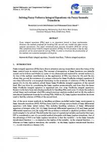
(26) The exact and approximate solution of Adomian method in this example at x = 0.5 and y = 0.5 for n = 3 are shown in figure 1.

j 0



Ti ( x, y)   Aij  j j 0

where β is a parameter introduced for convenience. By substituting (26) and (27) in (25), we have:

(27)

42572

Kirtiwant P Ghadle and Ahmed Abdullah Hamoud./ Elixir Appl. Math. 98 (2016) 42567-42573

Figure 1: Compares the exact and approximate solutions. Figure 2: Compares the exact and approximate solutions. Example 2. In this example, the method in this paper will be applied by the Mathematica 5.0 software package. Consider the fuzzy Fredholm-Volterra integral equation as follows:

where

Conclusion We solved fuzzy Volterra-Fredholm integral equations by using ADM was converted to a system of Volterra-Fredholm integral equations. In this paper, the ADM has been successfully employed to obtain the approximate solution of the fuzzy Volterra-Fredholm integral equation. For this purpose, in examples we used ADM to find the approximate solution of this system and hence obtain an approximation for fuzzy solution of the fuzzy Volterra-Fredholm integral equation, are used to solve the linear and nonlinear system. The iterative method conjugate gradient method and Homotopy analysis method are proposed to solving the fuzzy Volterra-Fredholm integral equation. References

by equations. (15 − 23) and (30 − 32) with

  102 , n  11, (t  0.3, 0  x  0.6). x

EXACT

APPROXIMATE (ADM)

0.1

0.2204663982

0.2203548375

0.2

0.3063488741

0.3062332542

0.3

0.4037996457

0.4035946723

0.4

0.5234862761

0.5233741235

0.6524855123

0.6523678927

0.6

Table 1: The exact and approximate solution of example 2.

[1] E. Babolian, H. Sadeghi Goghary, S. Abbasbandy: Numerical Solution of Linear Fredholm Fuzzy Integral Equations of the Second kind by Adomian Method, Appl. Math. Comput. 161 (2005), pp. 733-744. [2] S. Seikkala: On the Fuzzy Initial Value Problem, Fuzzy Sets and Systems, vol. 24, no. 3, (1987), pp. 319-330. [3] B. Bede, S. G. Gal: Generalizations of the Differentiability of Fuzzy Number-Valued Functions With Applications to Fuzzy Differential Equations, Fuzzy Sets and Systems, vol. 151, no. 3, (2005), pp. 581-599. [4] Y. Chalco-Cano, H. Roman-Flores: On New Solutions of Fuzzy Differential Equations, Chaos, Solitons and Fractals, vol. 38, no. 1, (2008), pp. 112-119. [5] D. Dubois, H. Prade: Towards fuzzy Differential Calculus. I: Integration of fuzzy Mappings, Fuzzy Sets and Systems, vol.8, no. 1, (1982), pp. 1-17.

42573

Kirtiwant P Ghadle and Ahmed Abdullah Hamoud./ Elixir Appl. Math. 98 (2016) 42567-42573

[6] C. X. Wu, M. Ma: Embedding problem of fuzzy number space. II, Fuzzy Sets and Systems, vol. 45, no. 2, (1992), pp. 189-202. [7] M. Friedman, M. Ming, A. Kandel: Numerical Solution of fuzzy Differential and Integral Equations, Fuzzy Sets and System, 106 (1999), pp. 35-48. [8] B. N. Mandal, S. Bhattacharya: Numerical solution of some classes of integral equations using Bernstein polynomials, Appl. Math. Comput, 190 (2007), pp. 17071716. [9] Kirtiwant P Ghadle , Ahmed Abdullah Hamoud: On the Numerical Solution of Volterra-Fredholm Integral Equations with Exponential Kernel using Chebyshev and Legendre Collocation Methods, Elixir International Journal, Appl. Math. 95 (2016), pp. 40742-40746. [10] G. Adomian: A Review of the Decomposition Method in Applied Mathematics, J. Math. Anal. Appl. 135 (1988), pp. 501-544. [11] N. Bildik, M. Inc: Modified Decomposition Method for Nonlinear Volterra-Fredholm Integral Equations, Chaos, Solitons and Fractals 33 (2007), pp. 308-313. [12] E. Babolian, J. Biazar, A. R. Vahidi: Solution of a System of Nonlinear Equations by Adomian Decomposition Method, Appl. Math. Comput. 150 (2004), pp. 847-854. [13] E. Babolian, A. Davari: Numerical Implementation of Adomian Decomposition Method, Appl. Math. Comput. 153 (2004), pp. 301-305. [14] S. Abbasbandy, T. Allahviranloo: Numerical Solution of Fuzzy Differential Equations by Taylor Method, Computational Methods in Applied Mathematics, 2 (2002), pp. 113-124.

[15] S. S. L. Chang, L. A. Zadeh: On Fuzzy Mapping and Control, IEEE Trans. Systems, Man cybernet, 2 (1972), pp. 30-34. [16] D. Dubois, H. Prade: Operations on Fuzzy Numbers, Int. J. systems Science, 9 (1978), pp. 613-626. [17] D. Dubois, H. Prade: Towards Fuzzy Differential Calculus, Fuzzy Sets and Systems, 8 (1982), pp. 1-7. [18] D. Dubois, H. Prade: Theory and Application, Fuzzy Sets and Systems. Academic Press, [1980]. [19] I. L. El-Kalaa: Convergence of the Adomian Method Applied to a Class of Nonlinear Integral Equations, App. Math. Comput. 21 (2008), PP. 327-376. [20] M. A. Fariborzi Araghi, Sh. S. Behzadi: Solving Nonlinear Volterra-Fredholm Integro-Differential Equations using the Modified Adomian Decomposition Method, Comput. Methods in Appl. Math. 9 (2009), PP. 1-11. [21] Yabin Shao, Huanhuan Zhang: Fuzzy Integral Equations and Strong Fuzzy Henstock Integrals, Hindawi Publishing Corporation Abstract and Applied Analysis, (2014), Article ID 932696, PP. 1-8. [22] T. Allahviranloo: the Adomian Decomposition Method for Fuzzy System of Linear Equations, Applied Mathematics and Computation. J, 163 (2005), pp. 553563. [23] A. M. Wazwaz: A New Algorithm for Calculating Adomian Polynomials for Nonlinear Operators, Appl. Math. Comput. 3 (2000), pp. 53-69. [24] K. Abbaoui, Y. Cherruault: Convergence of Adomians Method Applied to Nonlinear Equations, Math. Comput. Model, 20 (9) (1994), pp. 69-73.