Int J Adv Manuf Technol DOI 10.1007/s00170-017-0586-5
ORIGINAL ARTICLE
Study of the machine parameters effects on the case depths of 4340 spur gear heated by induction—2D model Noureddine Barka 1
Received: 14 March 2017 / Accepted: 24 May 2017 # Springer-Verlag London 2017
Abstract This paper presents the sensitivity study applied to spur gear heated by induction-heating process by exploring the effect of machine parameters on the hardness profile. The main process parameters, including the power (kW), the heating time (s), and the generator frequency (kHz) are the basic parameters that affect greatly the hardness and ultimately the mechanical performances. This research is made possible by simulation results obtained by coupling electromagnetic field and heat transfer. In order to complete the analysis, three stages are required; first, a Comsol 2D model was built considering the material properties and the machine parameters. Second, the surface temperatures and the case depths are deeply analyzed with the variation of the machine parameters. The relationship between the imposed current density in the coil and the power provided to the heated part is also determined. Finally, the sensitivity of hardness profile with the machine parameters variation was investigated using various statistical tools. Keywords Induction heating . Gear . Hardness profile . Sensitivity study
1 Introduction Industrial application of induction hardening is a potent and precise process that aims to enhance the mechanical and tribological properties of the steel parts [1, 2]. It consists in heating specific regions of a part above the austenitizing * Noureddine Barka
[email protected] 1
Département de mathématiques, d’informatique et de génie, Université du Québec à Rimouski, Rimouski, Québec G5L 3A1, Canada
temperature (Ac3) to allow martensite to be formed after quenching. The control of hardness profile is a must to improve wear resistance and increase contact fatigue life while keeping the part core unaffected [3, 4]. Induction hardening process is a result of electromagnetic, thermal, metallurgical, and mechanical phenomena that implies few physical fields. Thereby, achieving the desired result requires a lot of preexperiments and metallographic analyses which obliges the practitioners to use trial and error methods to develop their components. In this case, the simulation plays a crucial role since it helps to approach the process first qualitatively and second quantitatively using the appropriate tests. Further, the numerical methods aid to understand and optimize induction hardening and facilitate process development and reduce largely the lead-time [5]. From literature survey, induction technology in general covers a wide range of research whether in heating, melting or (and in) hardening fields [6, 7]. Focusing on the hardening process, the majority of relevant researches were about modeling the hardening process in order to study the hardness profile and the residual stresses distribution of the different parts [8–10]. Using actual induction machine, the important control parameters are the input power (PM) expressed in kilowatt, the heating time (s), and the generator frequency (kHz) [11, 12]. The same parameters are used in simulation except the initial current density (J0) expressed in ampere per square meters that replaces the machine power. Consequently, the relationship between J0 and PM is found during previous research and has permitted to determinate the power ratio [13, 14]. In fact, the ratio is calculating between consumed power obtained by simulation and real input power provided by machine basing on the same hardness profiles in simulation and experimental test and keeping on the same heating time and frequency. It remains to prove the effects of these parameters on the hardness profile using only simulation after verifying that the
Int J Adv Manuf Technol
simulation models are general in other operating condition. Then, without doing more experimental tests on the induction machine, the simulation models developed using Comsol are able to study the effect of parameter variation and finally the sensitivity of hardness profile under the effect of each one. The process of induction hardening has been carried out for many years and by many researchers whether by experimentation or simulation. However, its application for studying the hardness profile sensitivity on the material or as a function of machine parameters is still rather rare. In addition, the effect of machine parameters on the hardness profile has never before been thoroughly covered and documented [14–18]. The previous researches are done mainly without referring to nonequilibrium conditions and believe that the behavior in equilibrium remains valid even under conditions where the heating and cooling is fast. In addition, the vast majority of applications are made at slow average heating rate and this problem has not been considered. This research aims to study the sensitivity of hardness profile by the variation of machine parameters. Indeed, the effects of various factors enable a comprehensive analysis of the process and really understand his behavior before converging toward trend models applied to spur gear 3D numerical simulation. In this sense, the 2D simulation results obtained using Comsol software were optimized and calibrated using experimental data. Then, the effect of the machine parameters on the case depth is analyzed and the sensitivity of the hardness profile is studied around specific hardness profiles and using experience design (DOE).
2 Simulation 2.1 2D model The 2D model used during this study allows to solve the thermal-electromagnetic coupling in order to calculate the temperature distribution in a spur gear made from low-alloy steel (AISI-4340) with ϕ 105.2 mm external diameter and 6.5 mm thick and 48 teeth. The 2D model includes a gear tooth as represented in Fig. 1. In this case, the material is considered homogeneous and isotropic and the initial ambient temperature is set at 20 °C. Magnetic isolation is observed at limits (1, 10), (10, 11), and (1, 11). Thermal insulation is imposed at limits (1, 10) and (1, 11). An ambient temperature of 20 °C is taxed to the limit (10, 11). The inductor is represented by a solid section of 30-mm-thick copper. The model components are surrounded by an environment with a dielectric permeability (μr = 1) and a vacuum permittivity (εr = 1). The energy lost by convection is assumed equivalent to the energy lost by conduction through the air at the interface room/ambient environment. The energy lost by radiation is considered neglected due to the short time of treatment.
Fig. 1 Schematic representation of 2D model applied to spur gear
To optimize the meshing size, a convergence study was conducted using the 2D model developed early. This study was consisted to refine the mesh size to stabilize the obtained temperatures and induced current density in the inductor and part using the two frequencies (MF and HF). The mesh size is 0.1 mm at the core and are thinner (0.025 mm) at the tooth contour and the inside inductor circumference. The final mesh is showed in Fig. 2 and contains 545,000 elements and 1,132,700 degrees of freedom. The imposed current density (J0) is adjusted to have a specific temperature at the gear surface. The two frequencies used are the medium frequency (MF) adjusted at 10 kHz and high frequency (HF) in the range of 200 kHz. Simulation results demonstrate clearly that the imposed current density (J0) affect greatly the induced current density and the temperature distribution in the heated part. As presented in Figs. 3 and 4, MF heating affects more the root region and HF the tooth tip. Consequently, when MF is applied, the induced current is dispatched deeply. It is easy to remark that a majority of the tooth is heated above 700 °C. However, when the HF power is adjusted, the induced currents are distributed along the tooth contour, but they generate much more heat in the tip and pitch diameter regions. Consequently, the heat generated heats the tip at about 1000 °C and the pitch diameter to over 900 °C while the temperature at the root region does not exceed 600 °C. It is important to note that the heating time is fixed at 0.50 s and J0 is adjusted to 2.50 × 10⁹ A/m2 for MF and 8.10 × 10⁹ A/m2 in the HF case to reach a reference temperature of 1000 °C. 2.2 3D model The 3D model is developed by coupling Maxwell’s equations and heat transfer equation with adopting specific boundary conditions and considering only a quarter of the tooth. That
Fig. 2 Optimal mesh used in simulation
Int J Adv Manuf Technol Fig. 3 Induced currents density (A/m2) and temperature (°C) for medium frequency
approach helps greatly to reduce the computation time and furthermore increase the accuracy of simulation results. The efforts done by Barka et al. [19] have permitted to add two flux concentrators having the same geometry than the principal gear but with half thickness. The boundary conditions, mesh characteristics, and operational conditions are presented in Fig. 5. In this case, the model includes gear, flux concentrators, coil, and environment. The model uses symmetric conditions that are resumed by electric insulation and thermal insulation. These useful conditions help to reduce the gear, the coil, and the flux concentrators into the half geometries. Moreover, the periodic conditions are advantageously exploited in order to reduce the complete model to a simplified quarter one. This strategy has demonstrated the pertinences in terms of computation time and then the possibility to increase the mesh quality. The gap between the gear and the flux concentrator (Gapz) is varied during this study and demonstrated that it is possible to reduce completely the edge effect with a good tuning of this parameter. To be able to conduct a reasonable comparison between 2D and 3D, it is important to keep the same heating time (0.50 s) and vary the imposed current density (J0) in the coil in both MF and HF heating cases. In this case, J 0 is adjusted at Fig. 4 Induced currents density (A/m2) and temperature (°C) for high frequency
2.55 × 10¹⁰ A/m2 in MF case (10 kHz) and 9.50 × 10¹⁰ A/ m2 in HF case (200 kHz). This adjustment allows reaching a so-called reference temperature fixed at 1000 °C. The imposed current densities are more important when 3D model replaces the 2D model due to the flux concentrator addition since they are made in the same central component material. The 3D simulations are presented in Figs. 6 and 7 where there is no gap between the gear and flux concentrators for MF and HF respectively. The obtained results demonstrate that the temperature is uniformly distributed according to the gear thickness and then the edge effect is completely canceled. In this specific case, the temperature distributions are quite similar in MF and HF cases. The simulation results are useful to understand the induction-heating process and to help induction-heating developers to rapidly identify the adequate selection of parameters for the process and then achieve the desired hardness profile. These obtained results can justify the use of 2D model instead of 3D model since the equivalence between the so long gear (2D) and uniformity was provided by the use of flux concentrator principle (3D). It is demonstrated also that the powers consumed by the heated gear (derived from integration computation) are sensibly the same when 2D and 3D models are compared in both MF and HF cases. This strategy, favoring 2D
Int J Adv Manuf Technol Fig. 5 3D model with flux concentrator—meshing [19]
instead of 3D model, holds its legitimacy because the computing time can decrease greatly while increasing the quality of the mesh and subsequently the accuracy of the results.
The induction-heating machines have been developed according to the evolution of power generators and gear geometries. The advanced realized in terms of high-frequency power generators in the mid-1950s led to the development of double frequencies pulse heating (DFPH). Consequently, this heating mode consists to heat a component by two sequential steps using appropriate powers and two available frequencies as illustrated in Fig. 8. The preheating is usually performed at
medium frequency (MF) while the final heating is performed at high frequency (HF) to adequately distribute heat according to the contour of the teeth. Then, the austenitized regions are transformed into hard martensite upon quenching. Finally, an induction tempering can be used in order to relax the residual stresses field, to give a dimensional stability, and to slightly decrease the hardness by considerably increasing the toughness of the material. Experimental validation is performed on the induction machine located at the École de Technologie Supérieure (Montreal, Canada). This machine is equipped with medium and high frequency power generators. The first one uses audio-frequency technology with solid-state converters operating at 10 kHz and providing a maximum power of 550 kW. The second is a thyristor radio frequency generator operating at 200 kHz and providing a maximum power of 450 kW. Thus, the maximum power developed by the two combined generators is about 1 MW. This machine is capable of
Fig. 6 Temperature distribution (°C) for Gapz = 0 mm a edge and b middle plan using MF [19]
Fig. 7 Temperature distribution (°C) for Gapz = 0 mm a edge and b middle plan using MF [19]
3 Preliminary validation 3.1 Machine parameters
Int J Adv Manuf Technol Table 1 Test
1 2
Fig. 8 Sequential heating cycle using MF and HF frequencies
modulating both frequencies using the simultaneous double frequency heating concept and it is a numerically controlled machine tool with two numerical axes (vertical displacement and spindle rotation). The control of the machine parameters during the processing steps is ensured by a real time monitoring (RTM) module, which controls the quality of the processing by checking whether the actual parameters are identical to those requested by the operator. A typical heating procedure includes three different sequences. The first sequence consists to execute MF preheating using a specific power during a first time. The second sequence is in the form of dwell time without power application. The third and final sequence is HF heating that ensures to transform the gear contour into austenitic microstructure. In order to better characterize the surface hardness profile after quenching, the case depths are measured at the tip (dT), at the pitch diameter (dP), and at the root (dR) as showed in Fig. 9. 3.2 Validation results The preliminary tests are done in order to validate and calibrate the simulation model. Then, it is possible to establish practical ratios related to the relationship between the
Preliminary validation tests using MF and HF powers Frequency (kHz)
10 200
0.50 0.50
Power (kW)
220 83
Case depth (mm) Tip
Pitch
Root
0 1.5
0 0.3
1.1 0
consumed power determinate by simulation and the machine power. Since the model is based on 2D formulation, the case depth is measured at middle plan that divide the tooth in that radial direction. In fact, this virtual plan divides the gear into two equal parts along the radial direction. Table 1 presents MF and HF tests. The MF and HF tests have the same time of heating. It is significant to note that the MF power is three times more important than the HF case. This fact can be explained by the skin depth effect that stipulates that currents are more concentrated in the HF case. In both cases, the powers are adjusted to create a case depth about 1.1 mm in the MF case and between 1 and 1.5 mm in HF case. The results are concordant with the simulation efforts since MF hardens only the root and HF transforms the tip into martensite. After performing these tests, the simulation is explored to generate the same hardness profile using simulation parameters. The experimental results were compared using the simulation results that seems an interesting tool to distinguish the regions heated by induction. Using the assumption that any region heated up to the value Ac3 becomes austenite and transforms into martensite upon cooling, it is possible to predict the hardness profile. Thus, the simulation results show that only the root region and a small region around are transformed into hard martensite (Fig. 10a) when the medium frequency is applied (MF). However, if HF is employed, only the tip region and a small area close to the pitch diameter are hardened (Fig. 10b). At this point, the results confirm the validation tests. The bright region is hard martensite (above 60 HRC), and the dark region is the initial region composed of tempered martensite. Figure 11 confirms a significant correlation between the simulation results and the experiments in both MF and HF cases.
(a) Fig. 9 Measurement of case depths
Heating time (s)
(b)
Fig. 10 Hardness profiles obtained by simulation. a Test 1. b Test 2
Int J Adv Manuf Technol Table 3
Validation experiments—tests 3–6
Test Machine parameters
3
(a)
4
(b)
Fig. 11 Hardness profiles obtained by experiments. a Test 1. b Test 2
5 6
3.3 Model calibration The simulation results are consistent with the experimental validation for both tests. However, to validate quantitatively these results, it is necessary to find the relationship between the imposed current density in the inductor (J0) and power machine (PM). In fact, power ratios between the machine power (PM) and the power consumed by the gear (PS) are determined. Table 2 provides values of power ratio for tests 1 and 2. This ratio is more important for HF (67%) compared with MF cases (39%). Both ratios are much lower in comparison to the ratios determined in the case of the disc using the 2D axisymmetric model [20]. This difference can be explained by the fact that the 2D model underestimates the power ratios due to the complexity of gear geometry. In addition, a linear relationship is established between the imposed current in the coil and the consumed power using the simulation effort. Then, it is possible to assign an imposed current in the coil equivalent to the required power machine. Knowing the power ratio and given the linear relationship between J0 and PS, it is effortless to determine the current density imposed to adjust in the inductor during simulation process. The developed models must now be verified using new tests that the heating time is different from tests 1 and 2 and using MF and HF. Initially, four tests were used to test the robustness of the models and the results confirm that the errors between the developed models and experiments do not exceed 0.2 mm (Table 3). In a second step, it is interesting to see how the models behave if the MF and HF frequencies are sequentially combined in the same heating sequence. Consequently, two other tests were performed and are presented in Tables 4 and 5. Then, the same recipes were used in simulation using the same power, heating time, and frequency to find the case depths and then validate model robustness. The obtained results demonstrate that simulation combined to practical tests can be used
10 kHz, 0.25 s, and 380 kW 10 kHz, 1.00 s, and 140 kW 200 kHz, 0.25 s, and 152 kW 200 kHz, 1.00 s, and 52 kW
PM (kW)
PS (kW)
Ratio
1 (MF) 2 (HF)
220 83
85 56
0.39 0.67
Predicted case depth (mm)
dT
dP
dR
dT
dP
dR
0
0
0.95
0
0
0.85
0
0
1.20
0
0
1.30
1.50
0.50
0
1.50 0.70 0
1.80
0.40
0
2.00 0.35 0
advantageously for the development of recipes intended to develop mechanical components by induction. Thus, as shown in Table 6, the hardened depths obtained by simulation are quite comparable to those obtained in experimental tests. These results clearly demonstrate that the ratios are very useful for calibration and preliminary models that have developed a predictive capability with an error less than 0.20 mm for the gear and for the material used.
4 Sensitivity study Following the experimental validation, it is necessary to perform a sensitivity study of the hardness profile obtained (nominal profile with case depth at the tip of 2.50 mm (dT) and case depth at the root of 0.50 mm (dR)) using a sequential dualfrequency heating. The heating cycle is composed of a MF sequence followed by a dwell time (0.1 s) and finally a HF step will follow. This study is performed locally by varying the parameters around the nominal profile machine (level 2). MF power is varied from 20 to 40 kW, and HF power is varied between 150 and 170 kW. The MF heating time is varied between 0.9 and 1.1 s while the HF heating time is varied between 0.2 and 0.3 s. Finally, the dwell time is varied from 0 to 0.2 s. Table 7 summarizes the influence factors and their levels used in the design of the experiment. It is significant to remember that all data are obtained by simulation. An orthogonal matrix (MO) based on the Taguchi method and corresponding to 16 simulations is used for this purpose and allows Table 4
Validation experiments—test 7
Sequence
Frequency (kHz)
Heating time (s)
PM (kW)
PS (kW)
MF heating Dwell HF heating
10 – 200
1.20 0.20 0.20
20 – 210
10 – 168
Table 2 Power ratios Test
Measured case depth (mm)
Int J Adv Manuf Technol Table 5
Validation experiments—test 8
Sequence
Frequency (kHz)
Heating time (s)
PM (kW)
PS (kW)
MF heating
10
0.50
78
38
Dwell
–
0
–
–
HF heating
200
0.50
65.5
60
the grouping of machine parameters and hardened depth calculated by simulation. The design factor is the model most commonly used in experimentation. However, its use leads to excessive costs, especially when the number of factors is considered important. In addition, due to lack of rehearsal, the reliability of results produced by the factorial design is uncertain. Using an experimental design based on strategies such as orthogonal arrays (OA) generally leads to efficient and robust fractional designs to acquire information statistically significant with a minimum number of tests. Given that five parameters at three levels each are considered, a full factorial design of experiments would include 125 different simulations. Since the mesh is very refined in order to ensure a good precision of calculations, each simulation takes more than 2 days to converge toward the solution. However, by employing an orthogonal array (OA) based on the basic Taguchi, the design that meets this problem is a L16 corresponding to 16 simulations using different machine parameters and for each test, the case depths are measured. The simulation results were statistically analyzed using two statistical indices, derived from ANOVA, the percent contribution, and the average effects of each factor [21]. Simulation results are summarized in Table 8. Note that the case depth at the tip is much more sensitive to changes in machine parameters compared to that measured at the root. It is not surprising to observe that the maximum case depth can be achieved with experiment 3 and the case depths increase with machine parameters such as the power and heating time. According to the analytic methods described directly above, the RSM model corresponding to the simulated case depth (dR) was established. ANOVA was performed with a stepwise mode, which could eliminate the insignificant terms automatically. Table 9 presents the detailed contents of Table 6 Case depths (mm) for test 7 and test 8—experimentation and simulation Test
7 8
Experimentation
Scratching parameters and their levels
Table 7
Simulation
dT
dP
dR
dT
dP
dR
2.90 2.50
– –
0.50 0.45
2.75 2.40
– –
0.45 0.40
Parameters
Code
Level 1
Level 2
Level 3
MF power (kW)
A
20
30
40
HF power (kW)
B
150
160
170
MF heating time (s) Dwell time (s)
C D
0.9 0
1 0.1
1.1 0.2
HF heating time (s)
E
0.20
0.25
0.30
statistical analysis. In this case, the both MF and HF powers (A and B) and the HF heating time (E) are all significant model terms. Also, it is clear that final HF heating time has the largest effect on the response value. On the other hand, MF heating time and dwell time have the least effect. One can remark that the interaction terms affecting the case depth are neglected. The coefficient of determination (R2) is mainly used to measure the relationship between simulation data and predicted data. This result means that the process interesting responses are controlled by the all-important input parameters. In this case, R2 is equal to 95.37%, proving a high correlation between simulation and predicted results. The predicted R2 of 86.90% is in reasonable agreement with the adjusted R2 of 93.06%. The standard deviation related to dR prediction model is evaluated at 0.0300. The RSM model corresponding to the case depth at tip (dT) was also established. Table 10 presents the detailed statistical analysis for this case. At first sight, it is clear that MF power, HF power (A and B) and HF heating time have the majority influence on dT. Also, it is clear that final HF heating time has the largest effect on the response value. On the other hand, MF
Table 8
L16 orthogonal array and simulation results
Test
A
B
C
D
E
dT
dR
1 2 3 4 5 6 7 8
20 20 20 20 30 30 30 30
150 160 170 160 150 160 170 160
0.9 1 1.1 1 1 0.9 1 1.1
0 0.1 0.2 0.1 0.2 0.1 0 0.1
0.2 0.25 0.3 0.2 0.2 0.3 0.25 0.2
1.8 2.7 3.5 2.1 2.1 3.2 3 2.4
0.3 0.55 0.7 0.4 0.4 0.7 0.6 0.5
9 10 11 12 13 14 15 16
40 40 40 40 20 20 20 20
150 160 170 160 150 160 170 160
1.1 1 0.9 1 1 1.1 1 0.9
0.1 0.2 0.1 0 0.1 0 0.1 0.2
0.25 0.2 0.2 0.3 0.3 0.2 0.2 0.25
2.3 2.3 2.4 3.1 2.75 2.3 2.2 2.5
0.55 0.45 0.5 0.7 0.55 0.45 0.5 0.5
Int J Adv Manuf Technol Table 9
ANOVA for case depth at root (dR)
Table 11
Percent contributions of machine parameters
Characteristic
Code DoF Sum of Squares F value P value
Characteristic
A
B
C
D
E
Error
MF power (kW)
A
1
0.010355
11.48
0.007
HF power (kW)
B
1
0.031250
34.65
0.000
dR dT
5.31 0.48
16.04 17.97
2.57 1.40
0 0.16
71.45 73.88
4.63 6.11
MF heating time (s) C Dwell time (s) D
1 1
0.005000 0.000000
5.54 0.00
0.115 0.451
HF heating time (s) Error
1 10
0.139219 0.009020
154.35
0.000
15
0.194844
E
Total
heating time and dwell time have the least effect. It is very interesting to remark that the C and D terms affect less the case depth but are not neglected like in the first analysis related to dR. The coefficient R2 is equal to 93.89%, proving a high correlation between simulation and predicted results. The predicted R2 of 84.76% is in reasonable agreement with the adjusted R2 of 90.83%. Adequate precision measures the signal to noise ratio. The standard deviation related to dT prediction model is evaluated at 0.1048. The contributions of machine parameters are presented via the statistical analysis variance. According to the results obtained, relying on the contribution value of each parameter (Table 11), the case depths are mainly affected by heating time and power in the HF step while the effects of MF power and heating time are less important, with negligible effect of dwell time. In addition, each depth is affected differently by the parameters. Machine parameters in HF contribute to them alone for more than 90% of the variation of dT and over 87% of the variation of dR although the machine parameters in MF account for less than 2% of the variation of dT and less than 8% of the variation of dR. There is a significant difference in the contribution values of the power and the heating time in HF, wherein the heating time contributes more than four times than the power, knowing that the variation of heating time parameter was in small range of time with 0.05 s of step, contrary to the parameters of the power where its variation was in a wide range with a step of 10 kW. Not to mention that this difference in contribution between the HF machine parameters was noticed in both of dT and dR. Table 10
ANOVA for case depth at tip (dT)
Characteristic
Code DoF Sum of Squares F value P value
MF power (kW) HF power (kW) MF heating time (s) Dwell time (s) HF heating time (s) Error Total
A B C D E
1 1 1 1 1 10 15
0.01547 0.57781 0.04500 0.00500 2.37615 0.19666 3.21609
0.79 29.38 2.29 0.25 120.82
Average effect graph presented in Figs. 12 and 13 shows that case depths are affected by machine parameters at different degrees. These results illustrate the relative contribution of different factors in the variation of dT and dR depths and offer the nature of their relationship. It is important to note that the effects of four factors have the same trends. Generally, the two case depths are low under low heating conditions (MF power—20 kW, MF heating time—0.9 s, HF power—150 kW, HF heating time—0.2 s). However, these two depths are high at high conditions (MF power—20 kW, MF heating time—1.1 s, HF power—170 kW, HF heating time—0.3 s). Overall, the two case depths increase with the powers and with the heating times. An analysis of variance using ANOVA method was carried out in order to assess the significance of each machine parameter and consequently to determine the optimum one. Moreover, the results shown by the ANOVA method makes it possible to evaluate the sensitivity of case depths at root and at tip. In order to evaluate the contribution and give the statistical levels of significance of the process parameters, the variance ratio or F value of each considered parameter was compared with the values from standard F tables. Therefore, it was concluded that within the investigated processing window, HF power and HF heating time have a significant effects on the resulting case depths up to 100% of confidence level. However, the effect of the MF heating time on the resulting case depths is less than 90% and less than 85% for dR and dT respectively. The other parameters had no statistical significance on the achievable case depths. As mentioned above, the ANOVA method results were used to perform a local sensitivity analysis to study the effect variation of machine parameters locally. This study was based on an experimental design using the orthogonal arrays OA to achieve the high efficiency of the Taguchi method, and, it used only simulation results based on models developed and calibrated.
0.396 0.000 0.161 0.625 0.000
Fig. 12 Effect of simulation parameters on dR
Int J Adv Manuf Technol
3.
4. 5. Fig. 13 Effect of simulation parameters on dT
5 Conclusion The paper presented a sensitivity study permitting to determinate the global effect of machine parameters on the hardness profile using the simulation. First, 2D simulations are reviewed and a complete comparison between the MF and HF heating cases was conducted to emphasize the electromagnetic and thermal effects. The developed models have to be validated by experimental tests to verify the robustness of model and its power prediction. In the current situation, the experimental validation and calibration gave the power ratios between the input machine power and simulation power required to achieve quantitative prediction. Thereafter, a sensitivity study of the hardness profile calculated by simulation was related to machine parameters using statistical tools in order to analyze the effects of all factors known to affect the hardness profile. The sensitivity study exhibits the main machine parameters and theirs effects on the hardness profile. The case depth is supposed at the medium plan since 2D simulation model does not able to predict the edge effect. An analysis of this effect is under investigation using 3D model and will be the topic of future publications. The variation range in terms of machine parameters proposed in this study is equivalent to machine resolution. In fact, according the monitoring system related to the machine, the very short time of heating obligate the machine to provide high power rapidly and that affect the quality of response in terms of time and power. The results are also affected by the geometrical errors due principally to alignment between part and coil and design error of the coil itself.
6.
7.
8. 9.
10.
11.
12.
13.
14. 15.
16.
17.
18.
19.
References 1.
2.
Grum J, Mater J (2001) A review of the influence of grinding conditions on resulting residual stresses after induction surface hardening and grinding. Processing Technol Proc 114:212–226 Dietmar H, Qingzhe L, Jonathan M-U, Dawid N, Thomas P, Alfred S, Schulz A (2016) Simulation of multi-frequency-induction-
20.
21.
hardening including phase transitions and mechanical effects. Finite Elem Anal des 121:86–100 Grum J (2000) Measuring and analysis of residual stresses after induction hardening and grinding. Mater Sci Forum 347-349: 453–458 Semiatin SL, Stutz DE (1987) Induction heat treatment for steel, second edn. American society of metal, Ohio Kai G, Xunpeng Q, Wang Z, Hao C, Zhu S, Liu Y, Song Y (2014) Numerical and experimental analysis of 3D spot induction hardening of AISI 1045 steel. J Mater Process Technol 214(11):2425– 2433 Eunkyung L, Brajendra M, Bruce R, Palmer (2016) Effect of heat treatment on wear resistance of Fe–Cr–Mn–C–N high-interstitial stainless steel. Wear 368-369:70–74 Patrice, Gouin O’ Saughnessey,. Martine, Dubé,. Irene Fernandez, Villegas. (2016) Modeling and experimental investigation of induction welding of thermoplastic composites and comparison with other welding processes. J Compos Mater, 0(0) 1–16 Rudnev V, Loveless D, Cook R, Black M (2003) Handbook of induction heating. Marcell Dekker Inc., New York Vincent S, Hossein M, Florent B, Philippe B (2015) Measurement and correction of residual stress gradients in aeronautical gears after various induction surface hardening treatments. J Mater Process Technol 220:113–123 Smalcerz, A. (2015) The use of multifrequency induction heating for temperature distribution control. Archives of metallurgy and materials, Vol 60, Issue 2. Jürgen F, Dietmar H (1999) Numerical simulation of the surface hardening of steel. Int J Numer Methods Heat Fluid Flow 9(6):705– 724 Magnabosco I (2006) Induction heat treatment of a ISO C45 steel bar: experimental and numerical analysis. Comput Mater Sci 35: 98–106 Kawagushi H, Enokizono M, Todaka T (2005) Thermal and magnetic field analysis of induction heating problems. Mater Process Technol 161:193–198 Callister WD Jr, Rethwisch DG (2008) Fundamentals of materials science and engineering. John Wiley, New York Favennec Y, Labbe V, Bay F (2003) Induction heating processes optimization a general optimal control approach. J Comput Phys 187(1):68–94 Yuan J, Kang J, Rong Y, Sisson RD Jr (2003) FEM modeling of induction hardening process in steel. Worcester polytechnic institute, MA Sadeghipour K, Dopkin JA, Li K (1996) A computer aided finite element/experimental analysis of induction heating process of steel. Comput Ind 28(3):195–205 Barka N, Bocher P, Brousseau J, Galopin M, Sundararajan S (2007) Modeling and sensitivity study of the induction hardening process. Adv Mater res 15-17:525–530 Barka N, Chebak A, El Ouafi A, Jahazi M, Menou A (2014) A new approach in optimizing the induction heating process using flux concentrators: application to 4340 steel spur gear. J Mater Eng Perform 23(9):3092–3099 Barka N, Bocher P, Brousseau J (2013) Sensitivity study of hardness profile of 4340 specimen heated by induction process using axi-symmetric modeling. Int J Adv Manuf Technol. 69:2747–2756 Ross PJ (1988) Taguchi techniques for quality engineering. McGraw-Hill, New York