Study of Trend-Stuffing on Twitter through Text Classification Danesh Irani, Steve Webb, Calton Pu
Kang Li
College of Computing Georgia Institute of Technology 266 Ferst Drive, Atlanta, Georgia
Department of Computer Science University of Georgia 415 Boyd GSRC, Athens, Georgia
{danesh,
webb, calton}@cc.gatech.edu
ABSTRACT Twitter has become an important mechanism for users to keep up with friends as well as the latest popular topics, reaching over 20 million unique visitors monthly and generating over 1.2 billion tweets a month. To make popular topics easily accessible, Twitter lists the current most tweeted topics on its homepage as well as on most user pages. This provides a one-click shortcut to tweets related to the most popular or trending topics. Due to the increased visibility of tweets associated with a trending topic, miscreants and spammers have started exploiting them by posting unrelated tweets to such topics – a practice we call trend-stuffing. We study the use of text-classification over 600 trends consisting of 1.3 million tweets and their associated web pages to identify tweets that are closely-related to a trend as well as unrelated tweets. Using Information Gain, we reduce the original set of over 12,000 features for tweets and over 500,000 features for the associated web pages by over 91% and 99%, respectively, showing that any additional features would have a low Information Gain of less than 10−4 and 0.016 bits, respectively. We compare the use of na¨ıve Bayes, C4.5 decision trees, and Decision Stumps over the individual sets of features. Then, we combine classifier predictions for the tweet text and associated web page text. Although we find that the C4.5 decision tree classifier achieves the highest average F1-measure of 0.79 on the tweet text and 0.9 on the associated web page content, we recommend the use of the na¨ıve Bayes classifier. The na¨ıve Bayes classifier performs slightly worse with an average F1-measure of 0.77 on the tweet text and 0.74 on the associated web page content, but its required training time is significantly smaller.
1.
INTRODUCTION
Twitter is growing in popularity as a micro-blogging service for users to share a short message (called a tweet) that contains a maximum length of 140 characters with friends and others. It grew to over 7 million unique visitors [17] and 50 million tweets per day [29] in 2009. Estimates as of February 2010 [4] put Twitter at 20 million unique visitors monthly and over 1.2 billion tweets a month. Technically, Twitter is a multicast service where followers subscribe to postings from users and topics [23] of interest. Twitter’s
CEAS 2010 - Seventh annual Collaboration, Electronic messaging, AntiAbuse and Spam Conference July 13-14, 2010, Redmond, Washington, US
[email protected] homepage contains listings of trending topics, which are associated with news related to current events or upcoming events, under the headings of: “currently popular,” “popular this hour,” and “popular today.” An abbreviated list of these topics is also found alongside most user pages. Trending topics help users receive the tweets they are interested in and allow visitors to catch up with the latest topics. Unfortunately, the keywords found in trending topics are increasingly misused by spammers and other miscreants to promote their own interests in a practice we call trend stuffing. Such a practice can be classified under the Web Spam Taxonomy [9] as a form of boosting with dumping. Typical scenarios of misuse include tweets that are unrelated to a trending topic’s meaning but include the necessary keywords to be associated with the topic anyway. These deceptive associations can be achieved easily by adding the hashtag – a word or tag prefixed with a ‘#’ character to identify topics – for a currently popular topic to the content of a spammy tweet. When unsuspecting followers of a targeted trending topic receive spammy tweets, they unknowingly click on spammy links, exposing themselves to unwanted and potentially dangerous web content. The practice of trend stuffing is against the rules outlined in the “Spam and Abuse” section of Twitter’s fair use policy [3], and tools have been introduced to combat such tweets [2, 8]. However, despite these efforts, trend stuffing continues to occur frequently on Twitter. Automated identification of tweets that contain trendstuffing is a significant challenge due to the limited amount of information contained within their 140-character limit. The first contribution of this paper is an approach to automatically identify trend-stuffing in tweets. Our approach consists of three important components. First, for each trending topic, we build a model that describes its associated tweet content. The goal of these models is to distinguish trend-stuffing tweets from legitimate tweets based solely on the limited content information provided by a tweet. Second, when a tweet contains a URL, we use the URL to build a meta-model of its web page content. This meta-model is effective since most spammy tweets aim to promote a website. Finally, we combine the tweet content models with the web page content meta-models to increase their discriminating power. The second contribution of the paper is a quantitative evaluation of the performance of each model and their combination using a data set of over 1.3 million tweets (collected between November 2009 and February 2010). This evalua-
tion data set includes the collection of web pages pointed to by the tweets, which consists of 1.3 million web pages after following any redirect chains that may have been present. Additionally, we also verified the longevity of the accounts responsible for sending those tweets. If an account has been suspended, we assume that it has been classified as a spammer or miscreant by Twitter. This information is used to sharpen our evaluation (e.g., to verify if tweets classified as “not belonging to a trend” are actually trend-stuffed tweets). When using individual single-trend classifiers, the C4.5 decision tree classifier achieves the highest average F1-measure of 0.79 on the tweet text and 0.9 on the associated web page content. After combining the classification predictions from the tweet text and the associated web page content, we find that the C4.5 decision trees perform the best when combined with the ‘OR’ operator, displaying a 0.9 F1-measure for combined classification. Combining the classifiers using simple ‘OR’ and ‘AND’ operators allows us to take advantage of the performance of the respective classifiers while “short-circuiting” the combined classification with a positive or negative prediction respectively.
2.
PROBLEM DESCRIPTION
Before we discuss the problem we are trying to solve, we briefly provide an overview of tweets and trending topics. Readers familiar with this subject matter can skip to Section 2.2.
2.1 Overview of Tweets and Trending Topics Tweets (or statuses) are short, 140-character messages that are posted by users in response to the question “What are you doing?”. A user’s tweets are delivered to all the friends following the user, and the tweets are also available on the user’s account. As the evolution of Twitter into an avenue for content-creation has steadily progressed, Twitter has changed the question posed to users (when posting a message) to “What’s happening?” [23]. Trending topics on Twitter are popular topics that are being tweeted about the most frequently at a particular point in time. As the question being posed to users is now “What’s happening?”, popular topics are usually associated with current events. In fact, some trending topics have played a significant role in providing news for breaking stories and allowing users to provide opinions on current events (e.g., Haiti disaster relief). Trending topics can be associated with global trends or local trends (based on local geographic events), but since global trending topics are more frequently targeted by spammers, we focus on them in this work. One final observation about trending topics is that they are often identified by hashtags – word or tags prefixed with a ‘#’ character.
2.2 Trend Stuffing Currently, trending topics are listed on the Twitter homepage as well as alongside most other pages on Twitter. Due to their high visibility, trending topics attract tweets that may not be directly related to the topic – a practice we call trend stuffing. These deceptive tweets may arise from spammers, marketers, or users who want to promote a particular message (e.g., “Happy Birthday Tim #worldcup”). Twitter’s Rules [3] forbid this behavior, stating permanent suspension will result from “post[ing] multiple unrelated updates to a trending or popular topic.”
Twitter has taken steps to reduce the amount of noise in trending topics [2, 8], and even though such measures have had an effect on the amount of obvious spam in the trending topics, it has not eliminated noise or spam completely. The exact details behind these measures have not been released, but when details have been released, spammers have found a way around them. For example, to avoid the detection mechanisms that take into account the history of a user’s tweets, spammers delete historic tweets (having only a few “non-deleted” tweets at a particular time). We further discuss some details of known measures used by Twitter in Section 6.
3. OUR APPROACH Our approach to trend stuffing can be split into three main steps. First, we study the use of text-classification based only on the 140 characters (or less) of the tweets. This analysis helps determine how useful the text of the tweets themselves is for building a classification model for a trend. Additionally, as we will discuss in Section 4, using over 12,000 features for the classification model is not feasible and requires an intermediary step to reduce the number of features considered for each trend. Second, we investigate text-classification based on web pages associated with tweets. The intuition is that the content of the web pages associated with tweets can also be used to determine if a tweet belongs to a trend or not. Further, this approach would likely be effective because spammers often promote websites by including URLs in their tweets. Once again, the number of website content features is too large (over 500,000) to be feasible for classification, and as a result, we employ an intermediary step of feature selection (discussed in Section 4) to reduce the number of features considered for each trend. The third step involves combining the text-classification results from the tweet text and the associated web page content. In particular, we compare the performance of using the ‘AND’ and ‘OR’ operators for combining the predictions from the tweet text classifier and the associated web page content classifier to determine whether the tweet (and associated web page) belong to a given trend. Before discussing the statistical methods used in our study, we describe the data set used for our experiments.
3.1 Dataset collection We gathered more than 1.3 million tweets that were related to 2,067 trends over a 3 month period between November 22, 2009 and February 21, 2010. The top 10 most popular trending topics were queried every hour using the Twitter API [1], followed by subsequently fetching tweets associated with the top 10 trends every minute. We also crawled all web pages linked by a tweet because tweets may contain little to no text with only a link promoting a site. In fact, since we are particularly interested in finding spammers or users who try to promote sites unrelated to a particular trend, we focus on tweets that contain links. We follow the link and its corresponding redirection chain to fetch the final web page belonging to the link. This collection process generated over 1.3 million web pages, not including intermediate web pages responsible for redirection. Further details on how we handle redirect chains as well as JavaScript redirection can be found in our previous work [25, 26].
The average size of a tweet in our data set is 105 characters, with a standard deviation of 9 characters. The average size of a web page linked to by a tweet is 55kB, with a standard deviation of 41kB. Although there are a number of other characteristics to explore, previous papers have already focused on characterizing Twitter [11, 13, 14, 15]. In this paper, we focus on the features used in classification and the actual classification itself. We perform text-classification on both the tweet text and the content of the final web page pointed to by the tweet. In both cases, we tokenize the text and use each word as a feature after performing Porter’s stemming [18], removing stopwords, and removing tokens with less than 50 occurrences throughout the dataset. The tweet text also undergoes additional pre-processing to remove any text that is directly associated with the trending topic (e.g., trend hashtags or words found to be part of the topic). Finally, we count the number of occurrences of the token and use this count as a numeric feature. After performing these steps, the tweet text generated over 12,000 features, and the web page content generated over 520,000 features.
3.2 Statistical Methods used in our Study We use a standard set of statistical classification methods in our study. We outline some important basic information about each statistical classification method as well as differences between the methods. Then, we detail the manner in which the classifiers are run along with our evaluation criteria. Readers familiar with standard classifiers can skip to Section 3.2.2.
3.2.1 Statistical Classification Methods We use a standard implementation of supervised machine learning algorithms from Weka 3.6.1 [30]. Table 1 lists the Weka classifiers used as well as the standard name of the algorithm implemented by the Weka classifier. We briefly discuss the classifiers below: 1. Na¨ıve Bayes is a standard classifier used with textclassification. Due to its strong assumption of independence between features, the classifier is fairly robust, even with a large set of features because it can independently assess each feature with respect to the class label. Further, the na¨ıve Bayes classifier can be easily trained as a passive or active learning classifier. 2. C4.5 decision tree is a standard decision tree classifier. The algorithm uses a small set of features, which most effectively split the class labels at each branch of the decision tree. The model created by a decision tree is easily readable and provides useful insight when analyzing results. 3. Decision Stump is a weak learner and can be thought of as a single-level “binary” decision tree. We use this to see how easily the class can be partitioned using a single feature. All classifiers are used with their default settings and are run with 10-fold cross-validation to avoid over-fitting. We provide a more thorough discussion of the benefits and drawbacks to using particular classifiers along with the results in Section 5. We use supervised learning because our initial experiments with an unsupervised learning algorithm (clustering
Classifier Na¨ıve Bayes J48 DecisionStump
Algorithm Type Na¨ıve Bayes C4.5 Decision Tree Decision Stump
Table 1: List of classifiers used with categorical features. using k-means) generated unsatisfactory results. Specifically, we found that the large number of features and sometimes irrelevant features caused the clustering algorithm to perform poorly. On the other hand, the supervised learning algorithms were able to quickly and accurately identify tweets not belonging to a given trend, even in the presence of noisy labels.
3.2.2 Statistical Classification Setup We build a classifier model for each of the 670 trends with over 200 tweets, using one-to-many classification with all the tweets belonging to the trend in one class and a stratified sampling of tweets in the other trends (with at minimum one tweet per trend). As an example, if a particular trend has 500 tweets, we pick 669 tweets from the other trends resulting in classification for 1169 tweets. We do not build one single multi-class classifier for multiple reasons: 1) retraining would be required for new classes (trends) and over time, as topic drift occurs; 2) smaller classifiers would be quicker and more robust; 3) more aggressive feature selection can be performed to reduce the feature set to only those terms relevant to the particular trend. As we are using supervised learning, we need to provide labels for training the classifier (or building the model). We use a label associated with each unique trend text (e.g., “welcome 2010” or “tiger woods”) as assigned by Twitter. When assigning labels, we do not remove tweets from suspended accounts from the data set because in practice, these algorithms will be trained on somewhat noisy data as tweets are only identified as “bad” after a certain time-lag. The classifiers will need to rely on the confidence bounds as well as cross-validation to only learn features of tweets related to the trend and ignore the noise. Although this decision might result in trends containing a large number of noisy labels such that the noise is included in the model of tweets belonging to the trend, this methodology represents a realistic scenario that we wish to analyze.
3.2.3 Evaluation Criteria of Statistical Methods on Data Sets We use F1-measure to evaluate and compare the results of the classifiers. The F-measure is a weighted harmonic mean between the precision and recall. To define this metric, we first need to review the possible outcomes of a single classification using a confusion matrix: Actual Label Trend Other
Predicted Label Trend Other True-Positive (TP) False-Negative (FN) False-Positive (FP) True-Negative (TN)
In our one-to-many experimental setup, positive tweets are tweets that belong to a given trend, and negative tweets are tweets that belong to other trends for the particular experiment. In our evaluation, we take into account the
Percentage of tweets from suspended accounts
(a) Average lowest Information Gain
100 90
Feature category
80
Tweet Text Web Page Content
70 60
(b) Average total feature set’s Information Gain
50 40
Feature category
30
Tweet Text Web Page Content
20 10
Number of features 100 1000 5000 2.1 2.5 14.6 46.9 70.9
0
10
10
10
0 00
0 00
00
0
Number of tweets
Figure 1: Percentage of suspended tweets vs number of tweets in a trend number of suspended tweets classified as positive. These tweets are incorrectly classified because as mentioned earlier, suspended tweets are likely to not belong to any trend. Precision is a measure of the fraction of actual positive tweets found by the classifier in relation to all positive tweets found by the classifier, given by TPTP . Recall is a measure + FP of the fraction of positive tweets found by the classifier in relation to all actual positive tweets, given by TP TP . + FN (1+β2)∗T P . The F1Finally the F-measure is given by β2∗T P +F P +F N measure is the F-measure with the value of β set to 1. As when calculating precision and recall, we take into account the number of suspended tweets and adjust the F1-measure accordingly.
3.2.4 Data Set Label Refinement To identify tweets associated with trend stuffing, we requeried the Twitter accounts of users who had tweets in our data set to check if their Twitter account had been suspended. We found over 26,000 Twitter accounts associated with tweets that had been suspended (or approximately 3.5% of all accounts collected), which were responsible for over 130,000 tweets (or approximately 10% of all tweets collected). We do submit that a very small percentage of these accounts may have been suspended for purposes other than spam, and in-addition, there are Twitter accounts that have been used for spam that have not yet been suspended by Twitter. Figure 1 shows the number of tweets in a trend on the x-axis, as well as the percentage of tweets in a trend which come from suspended accounts on the y-axis. Each point represents a unique trend.
4.
Number of features 100 1000 5000 0.004 < 10−4 0.096 0.016 0.002
REDUCTION OF FEATURE SETS
Classification with over 12,000 features for the tweet text and over 520,000 features for web page content is not practical. Most classifiers will perform poorly either due to the curse of dimensionality [6] or due to the computational burden of trying to analyze patterns associated with all the features (e.g., in Neural Networks learning weights for thousands of input nodes). We chose Information Gain to reduce the number of features to a tractable size. Information Gain, from an information theoretical perspective, is a measure of the amount of expected reduction in entropy if one were to use the fea-
Table 2: Comparison of the number of features considered, when using Information Gain to reduce the feature set size.
ture to partition tweets belonging to a trend from tweets not belonging in a trend. After calculating the amount of Information Gain for each feature, we pick the strongest features. Previous work on a study of feature selection in text categorization [31] found that Information Gain was effective in drastically reducing (by up to 98%) the number of features used for classification while not losing categorization accuracy. As we plan to do the feature selection for each trend when performing one-to-many classification, we believe an even more drastic reduction can be preformed. We decided to evaluate our classification with a more tractable set of 100 and 1000 features for the tweet text – 0.8% and 8% of the total number of tweet text features, respectively – and a set of 100, 1000, and 5000 features for the web page content – 0.02%, 0.2% and 1% of the total number of web page content features, respectively. Table 2 shows the average lowest Information Gain and the average total Information Gain. The average lowest Information Gain is the average Information Gain of the weakest feature in the feature set, and it indicates that any features not added into the set will have an Information Gain value lower than it. The average total Information Gain can intuitively be thought of as the average total discriminative power of all the features used to distinguish the trend from others. For the tweet text from the Table 2(a), we see that after 100 features, the average Information Gain of the weakest feature drops to 0.004, which is indicative of most of the discriminative power being captured in the first 100 features. This is further shown in Table 2(b) where the average total Information Gain increases by only 0.4 when considering an additional 900 tweet text features. In fact, we find that on average, after 317 features, the Information Gain drops to zero. For evaluation purposes, we still consider tweet text classification both using 100 and 1000 features. For the web page content from Table 2(a), the average Information Gain of the weakest feature when considering 100, 1000, and 5000 features is 0.096, 0.016, and 0.002, respectively. Considering the average total Information Gain shown in Table 2(b), we see a 300% increase from 100 to 1000 features and a further 50% increase from 1000 to 5000 features. The large increase in entropy when considering web page content features (especially when going from 100 to 1000 features) makes it likely that using 100 features for classification for web page content may not be enough. We will evaluate web page content classification using 100, 1000, and 5000 features.
1 0.9 0.8 F1−measure
0.7 0.6 100 1000
0.5 0.4 0.3 0.2
Tweet text Training Time (ms) Na¨ıve Bayes C4.5 Decision Tree DecisionStump Test Time (ms) Na¨ıve Bayes C4.5 Decision Tree DecisionStump
Number of features 100 1000 0.21 0.79 0.77 7.80 0.22 0.86 100 1000 0.26 1.12 0.08 0.11 0.07 0.11
0.1 0
Naive_Bayes
Table 3: Average time in ms, to train and test the classifiers over the tweet text.
C4.5_Decision_Trees Decision_Stump Classifiers
Figure 2: Results of classification on tweet text using different number of features. Error-bars represent one standard-deviation of the F1-measure. 1
F1-Measure
0.8
0.6
0.4
0.2
0
0 00
0 10
00
0 10
0
0 10 Number of Tweets
Figure 3: F-measure of na¨ıve Bayes classifier using 100 tweet text features.
5.
EXPERIMENTAL CLASSIFICATION RESULTS
We separately evaluate the effectiveness of classification on the tweet text and the web page content. Then, we evaluate combining the predictions of both classifiers. As previously mentioned, we use tweets from suspended accounts to validate the false-negatives. Validating the true-positives requires a larger manual effort, and we explore this approach for a subset of tweets in Section 5.4. As a baseline for our classification results, we use the majority classifier, which classifies all profiles into the larger class. The class representing a sample of all tweets except tweets na¨ıvely classified into the trend has the same size as the opposing class so both classes have an equal size. The majority classifier would have a 50% accuracy with a F1measure of 0.66 (assuming the positive class is assigned the majority class) or 0 (assuming all tweets are majority classified into the negative class) – for our purposes, we use a baseline F1-measure of 0.66. All experiments were run on Redhat Enterprise Linux using a 3 Ghz Intel Core 2 Quad CPU (Q9650) with 8 GB RAM.
5.1 Classification using Tweet Text We first look at the results of the classifiers that use only features based on tokens in the tweet text. The results of
classification using these features is shown in Figure 2. Each set of bars represents a different classifier, and each bar within the set represents the average performance in terms of F1-measure on a different number of features. We see that na¨ıve Bayes and C4.5 decision trees perform well, with C4.5 decision trees performing the best by a small margin. Decision Stumps, on the other hand, perform even worse than the baseline majority classifier. C4.5 decision trees and na¨ıve Bayes have the highest F1measure as they have a lower number of false-negatives (tweets classified as not being in the trend). Decision Stumps are only able to use a single feature to decide if a tweet is in the trend or not, and in the absence of a “hashtag,” it is not able to perform very well. The poor performance of Decision Stumps was due to the low expressive power of a single Decision Stump and lack of a single feature that could, without noise, capture the essence of a trend. Compared to a sample of C4.5 decision trees, we found the root node to be the same, but the C4.5 decision tree had a number of branches under the root to filter out false-positives and false-negatives. Figure 3 shows the F1-measure results of na¨ıve Bayes classification using 100 features. The number of tweets belonging to the trend being classified (the positive class) is shown on the x-axis with the F1-measure on the y-axis. We see that as the number of tweets in the positive class increases, the amount of variation in the F1-measure reduces significantly with the scores tending to be higher. The reason for this is that some of the positive classes may contain a large percentage of noise (suspended tweets); this is especially true for smaller trends. If this is the case, the classifier learns the noise as part of the trend. In calculating the F1-measure, since we consider suspended tweets not part of the trend, this can reduce the resulting F1-measure. As the number of tweets in the positive class increases, the likelihood of noisy tweets being classified as part of the trend decreases, resulting in fewer false-positives (i.e., tweets that were suspended and thus not part of the trend, being classified as positive). The reason for the small difference between the classification using 100 features and 1000 features of tweet text is likely due to the Information Gain per feature being very low after selecting the strongest 100 features (in some cases even zero). One of the other important factors in the performance of a classifier is the amount of time it takes to build the model and the time it takes to classify a tweet. Table 3 shows the result of the average model build time (training time) and average classification time (test time) for a single tweet for both 100 and 1000 features using different classifiers. We
1
F1−measure
0.8 0.6
100 1000 5000
0.4 0.2 0
Naive_Bayes
Number of features 100 1000 5000 0.17 1.19 7.06 0.62 9.46 781.90 0.17 1.25 7.53 100 1000 5000 0.17 0.90 5.96 0.05 0.11 0.19 0.05 0.13 0.39
Table 4: Average time in ms, to train and test the classifiers over the web page content.
C4.5_Decision_Trees Decision_Stump Classifiers
Figure 4: Results of classification on web page content using different number of features. Error-bars represent one standard-deviation of the F1-measure. 1
0.8
F1-Measure
Web page content Training Time (ms) Na¨ıve Bayes C4.5 Decision Tree DecisionStump Test Time (ms) Na¨ıve Bayes C4.5 Decision Tree DecisionStump
0.6
0.4
0.2
0
0
0 00
10
0 00
10
00
10 Number of Tweets
Figure 5: F-measure of C4.5 decision tree classifier using 100 web page content features. see that Decision Stumps take the least time for both building the model and to classify a tweet, but this is due to the very simplistic single branch model. Na¨ıve Bayes is faster at building a model than C4.5 Decision Trees because in na¨ıve Bayes, each feature is treated independently and thus can be looked at once. On the other hand, when building a C4.5 decision tree, at every node an attribute is picked based on the highest Information Gain of available features, followed by a recursion on the smaller subtrees. C4.5 decisions trees are much faster than na¨ıve Bayes on classifying a tweet once the model is built because a relatively small decision tree needs to be traversed to determine a label for the tweet. Conversely, na¨ıve Bayes needs to calculate the combined sum of probabilities for all the features. This requirement is the reason there is an over 400% increase in time taken when using na¨ıve Bayes to classify a tweet with 100 features versus 1000 features.
5.2 Classification using Web Page Content We now explore the classification of tweets based on the text features from the web page content associated with the tweets. Web page content associated with tweets should also be related to the trend or be separable in such a way. The results of classification using these features is shown in Figure 4. Similar to Figure 2, each set of bars represents a different classifier, and each bar within a set represents
the average performance in terms of F1-measure using a different number of features. The C4.5 decision trees perform the best, followed closely by Decision Stumps. Na¨ıve Bayes performs the worst but better than a baseline classifier. C4.5 decision trees perform the best as they have the smallest number of false-negatives, followed by the Decision Stump classifier. The tree-based classifiers (C4.5 decision trees and Decision Stump) perform well in this case as there are a few strong features, which distinguish the trends. The explanation for this is that web pages related to the trend contained words strongly related to the topic. For example, the strongest features for the hashtag “#helphaiti” were “haiti”, “earthquake”, “donate”, “disaster”, and “relief”. The Decision Stump, due to the single level tree, cannot reduce the number of false-positives using further decisions. Figure 5 shows the F1-measure results of using the C4.5 decision tree classifier with 100 features on the web page content. The number of web pages belonging to the trend being classified (the positive class) is shown on the x-axis with the F1-measure on the y-axis. Similar to classification using tweet text, we find that the variance is lower and the F1-measure higher as the number of positive web pages increases. The reason for this is that as the trend size increases, the percentage of suspended tweets that make up a trend decreases, causing the classifier to be less likely to learn the suspended tweets as part of the trend. We also look at the time (ms) taken to build the classification models and to classify individual web pages. Table 4 shows the average time to build the model (training time) and time to classify (test time) a single web page using different classifiers and number of features. We see that the training time for na¨ıve Bayes and Decision Stumps are the lowest, and C4.5 decision trees take the most time. In terms of classifying a web page once a model is built, both C4.5 decision trees and Decision Stumps are the fastest, while the na¨ıve Bayes is relatively slow. The time the na¨ıve Bayes takes to classify a single web page associated with a tweet increases by over 600% when increasing the number of features from 1000 to 5000 features.
5.3 Classification using Tweet Text and Web Page Content Combined After studying the performance of the classifiers on the individual sets of features, a natural next step is to combine the predictions from the classifiers of the tweets and associated web pages to a combined prediction. There are two main reasons for doing so: 1. Tweets might not contain enough text to make an accurate classification all the time. Some tweets might
1
1
0.8
Naive_Bayes C4.5_Decision_Trees Decision_Stump
0.4 0.2 0
0.6 Value
F1−measure
0.8
0.6
0.4
Naive_Bayes
C4.5_Decision_Trees Decision_Stump
0.2
OR combined predictions using 100 features
0.8 F1−measure
00 00 10
0 00 10 Number of Tweets
Figure 8: F-measure of combined classifier using na¨ıve Bayes with 100 features on the tweet-text and C4.5 with 100 web page content features.
1
0.6
Naive_Bayes C4.5_Decision_Trees Decision_Stump
0.4 0.2 0
0
00 10
Figure 6: Results of F1-measure based on prediction from tweet text and web page content classifier combined using the ‘OR’ operator.
Naive_Bayes
C4.5_Decision_Trees Decision_Stump
AND combined classifiers using 100 features
Figure 7: Results of F1-measure based on prediction from tweet text and web page content classifier combined using the ‘AND’ operator. only contain a URL and a hashtag associating it with a trend. In this case, classifying the web page content associated with the tweet might help make an accurate classification on whether or not the tweet actually does belong to the trend. 2. It might be easy for a spammer to camouflage a tweet to look like it belongs to a trend, but it would take more effort (on the part of the spammer) to also camouflage the web page linked in the tweet to look like it belonged to the trend. Even if the spammer were to do so, they would have to customize their web page for each trend that they wish to spam, and this would likely be prohibitive. We compare two methods of combining the classification results from tweets and from the associated web pages, outlining possible improvements to this method in Section 5.5. The ‘AND’ and ‘OR’ operator are commonly used to check if results from two statements agree or disagree, and in the case of combining classification results, we will use these to check if the prediction over a tweet matches the prediction over the associated web page content. In the case of the ‘AND’ operator, we will mark a tweet as belonging to a trend, if the prediction for the tweet ‘AND’ the prediction for the web page associated with the tweet both predict that the tweet belongs to the trend. In the case of the ‘OR’ operator, we will mark a tweet as belonging to a trend, if either prediction for the tweet ‘OR’ prediction for the web page associated with the tweet predict that the tweet belongs to the
trend. Intuitively, by using the ‘AND’ operator, we ensure that both predictions on text and associated web page agree to classify it in the trend, causing an increase in the number of false-negatives and true-negatives. On the other hand, the ‘OR’ operator, will cause an increase in the number of true-positives and false-positives. Figure 6 and Figure 7 show the results based on combined classification using the ‘OR’ operator and ‘AND’ operator, respectively. The x-axis displays the classifier used for the tweet text, whereas each bar within a cluster denotes a classifier used to predict the label for the associated trend. All classifiers were trained and tested using 100 features. The y-axis shows the value of the F1-measure achieved by a combined tweet text and web page content classifier. We find that the combined classifier using the ‘OR’ operator performs better on average than the combined classifier using the ‘AND’ operator. As previously mentioned, this result is due to the ‘OR’ operator leading to more truepositives and perhaps even a few more false-positives and performing better than the best individual 100 feature classifier used. One of the possible reasons for not achieving results closer to 1 is likely due to trends which are largely made up of suspended tweets. We are currently investigating this further. In the case of combining classifiers using the “AND” and “OR” operator, both classifiers would have to be trained on the trend, and at least one of them would have to be probed at the time of making the determination of whether the tweet and associated web page belong to the trend. This is similar to the common practice of short-circuiting boolean expressions. In the case of an “AND” operator, a single negative prediction will result in the final label being negative, whereas in the case of the “OR” operator, a single positive prediction will result in the final label being positive. In respect to the tweets, the tweet text would be easier to get a classification label for, especially since obtaining a classification for the web page would involve fetching the destination web page followed by tokenizing and feature reduction of all the web page content. Thus, the minimum required time to classify a tweet using the combined approach is the time taken to classify the tweet text plus an estimated 21 of the time taken to classify the web page content (not taking into
account time to fetch, tokenize, and reduce features).
5.4 Manual Verification of a Subset of Results In our manual vetting of the results we reviewed a few hundred tweets and associated web pages. We make a number of interesting observations based on what we found: 1. Some spammy tweets had legitimate looking tweet text (they were “camouflage tweets”), but the link pointed to a web page that was unrelated to a trend. An example of this is the tweet “NFL Sunday Night Betting Preview - Brett Favre vs. Kurt Warner (maybe) [URL removed]” that was related to the trend “NFL” while linking to web page content for the dating site “Friend Jungle.” 2. Many of the false-negatives were tweets properly classified as not belonging to the trend. The reason they were counted as false-negatives is that they belonged to Twitter accounts not yet suspended. For example, the tweet “My Top 3 Weekly - Play Free Online Games [URL removed]” and associated web page were both classified as not belonging to the “My Top 3 Weekly” trend, but the Twitter account associated with this tweet had not been suspended yet. 3. Some false-positives belonged to a trend but were posted by suspended accounts. These were actually tweets and web pages to legitimate content related to a topic that used inappropriate or obscene language. An example is the tweet “Check this - Nicole Parker-Best of Britney Spears Part 2 [URL removed] Plz ReTweet! #musicmonday” related to the trend “#musicmonday” that links to a parody video of Britney Spears. It is likely that the account posting this tweet got suspended for the sexually suggestive content of the parody.
5.5 Overall Discussion C4.5 decision trees perform the best and would likely be resilient to a certain amount of adversarial interference, but the time taken to build a model for a C4.5 decision tree is a hindering factor in using such classifiers. The Decision Stump classifier performs quite well and can be trained very quickly, but it can be easily defeated by adversaries. Na¨ıve Bayes is the most robust, but it takes the longest when classifying each tweet. An advantage of the na¨ıve Bayes classifier is its suitability for online-learning; namely, it can be updated based on user feedback without a large re-training time. Therefore, we believe that using na¨ıve Bayes with a 100 features (or perhaps fewer, depending on the maturity of the trend) would be ideal in classifying tweets and their associated web pages. We plan on studying the applicability of using varying feature set sizes based on the number of tweets belonging to a trend as well as the effect of classifying recurring or multi-day trends. Working with 140 characters of text or less has been both beneficial and challenging in that we find that for a particular trend, a small selection of features are adequate in being able to accurately capture tweets belonging to a trend. On the flip side, the challenge is that as tweets contain pointers to allow gathering of further information, it is very easy for a spammer or a miscreant to camouflage the tweet (i.e., make the tweet text look legitimate while making the link
point to a spammy web page). It is due to this possibility that we also crawl web pages associated with tweets and use such content in our classification.
6. RELATED WORK Twitter has largely been studied for its network characteristics and structure. The largest such measure to date has been done by Kwak et al. [15] who study over 106 million tweets and 41.7 million user profiles. They investigate network characteristics ranging from a basic follower/following relationships to homophily (tendency for similar people to associate with one-another) to pagerank. They also study trends in relation to the similarity to topics on CNN and Google Trends, further characterizing most trends as being active. Huberman et al. [11] and Krishnamurthy et al. [14] also study the characteristics of Twitter, with the latter identifying users, their behaviors as well as geographic growth patterns. Java et al. [13] did an earlier study on the Twitter network a year after its growth and used the network structure to categorize users into three main categories: information source; friends; and, information seeker. Information sources they note, were “found to be automated tools posting news and other useful information on Twitter”. In terms of spam detection on Twitter, Yardi et al. [32] looked at the life-cycle and evolution of a trend, with focus on spam. Although they do identify some behavioral characteristics that can be used to identify spammers, they do concede that such behavioral patterns do come with their falsepositives. We plan to investigate if we could combine such techniques to come up with a robust technique to keep spam messages out of trending topics. Other attempts at spam detection on Twitter include, Spamdetector [24], which is a tool to apply “some heuristics to detect spam accounts”. Details on this project are unavailable, but their effort is continuing based on users’ feedback to bots on Twitter. Twitter themselves have taken a proactive approach to detecting spam on their network. In as early as July 2008 [21] and August 2008 [22], Twitter acknowledged an online battle with spammers and seemed to respond with placing limits on followers and delete spam accounts by using the “number of users who blocked a user” as feedback. Further steps were taken in November 2009 [8] and in March 2010 [10], first in relation to reducing the amount of clutter posted to trends (although details on their approach are limited), and second in relation to introducing a URL filter for protecting against phishing scams. There has been a lot of related work [20] on using textbased classification on e-mails to classify them as spam and non-spam. Such techniques could be directly applied to Twitter, but due to the short messages and camouflage to get users to click links in such posts, we believe that such techniques would have limited success. Our previous work [12] on classification of Social Profiles in MySpace is a precursor to this work, as that looks at zero-minute classification of social profiles using static profile information (features such as Age, Interests, and Relationship Status were used). As Twitter gathers very little information from a user during account creation, the previous technique would likely need to be applied in conjunction with other techniques, such as the one being proposed in this paper, to increase accuracy. Finally, over the past few years, we have performed an extensive amount of research on the general security challenges facing the social Web. We began by enumerating the various
threats and attacks facing social networking environments and their users [28]. Then, we turned our attention to one of the most pressing threats against the social Web: deceptive profiles. In [27], we presented a novel technique for collecting deceptive profiles (social honeypots), and we performed a first-of-its-kind characterization of deceptive profile features and behaviors. Next, using the profiles we collected with our honeypots, we extended our analysis and incorporated automated classification techniques to distinguish between legitimate and deceptive profiles [12, 16]. In this paper, we have complemented these previous efforts and helped to improve the quality of information in another important social environment.
7.
CONCLUSION
In this paper, we study the non-trivial problem of text classification in a restricted environment of only 140 characters, such as that presented by trend stuffing on Twitter. Our approach to the problem included first modeling tweets that belong to a trend using text-classification on the text of the tweet itself. We followed this with building a metamodel for web pages linked in tweets that belong to a trend. Finally, we combined both the tweet text model and the web page content model to increase the performance in classifying tweets that belong to trends. In each of the steps, we use additional information about suspended tweets to validate our results. To make text-classification on the tweet text and the web page content feasible, we first used Information Gain to reduce the number of features from over 12,000 and over 500,000, to less than 1,000 features and less than 5,000 features, respectively. For tweet text features and the web page content features, this accounted for a reduction of over 91% and 99%, respectively. We found that even with reductions this large, the Information Gain of additional features to be on the order of a thousandth of a bit. C4.5 decision trees achieve the highest F1-measure on both the classification of tweet text and associated web page content, resulting in an F1-measure of 0.79 and 0.9, respectively. Na¨ıve Bayes performs well on the tweet text with a result of 0.77 and not very well on the web page content. On the other hand, Decision Stumps perform well on the web page content with an F1-measure of 0.81 and not very well on the tweet text. We find by combining predictions from classifiers on the two sets of features, we perform well on most combinations of classifiers in the case of the ‘OR’ operator. In most cases, we do not find a significant difference between classification using 100 features and over a 1000 features. In addition we also compare the time taken to build a classification model and to test tweets or web pages against each classifier. We find that C4.5 decision trees take the longest to build a classification model but are very quick at testing an instance. Na¨ıve Bayes takes a much shorter time to build a classification model but takes longer at testing each instance.
8.
FUTURE WORK
Current performance of the combined classifiers could be improved by using classifier combination similar to the Bayesian combination technique used in our previous work [7]. The idea essentially being to adjust the weight of the classifier by the confidence of the classifier, or the amount of information (text or content) that is available to it. The root of
the combination technique is represented by the formula: X P (ω|x) = P (ω|Zi , x)P (Zi |x) i
Here ω is the probability of a trend given a tweet x, which results in the summation of the tweet text and web page classifiers, distinguished by the subscript i. P (Zi |x) is the classifier’s confidence given tweet x, which can be a simple measure of how much text is provided to the classifier or used to ignore the classifier in case the set of features it uses becomes unavailable. For example, certain tweets might only contain a link and no text, this would result in P (Ztweet−text |x) being zero or close to zero, whereas if the web page contained a lot of text, P (Zwebpage−content |x) would be close to 1. P (ω|Zi , x) is the posterior probability of ω given a single classifier and x. Further details of this method of combination and applying it to a disjoint set of features can be read in Section 4.2 of the previous work. In terms of scalability, one of the issues already addressed has been the training/testing times of the classifiers. Due to the large volume of Tweets and possible large number of models which will need to be stored, the question of further enhancements to the performance of classifiers does arise. In regards to the amount of space required for such classifiers, using “Mini”-filters [19] could be investigated as well as discarding models after a set period of time. The hashing trick [5] alternatively might useful in reducing the number of features considered by hashing features onto a fixed size hash (possibly eliminating the need for using InformationGain for attribute selection). Currently we use all the tweets belonging to a trend for training followed by classification, allowing cross-validation to partition the data. Further study is required to determine a threshold for the number of tweets required to build a classification model, followed by a time-interval for updating the model due to topic-drift. To validate our experiments further, as previously mentioned, we would like to manually label a large set of the tweets in a one-to-many setting, with each tweet and web page receiving labels from at least 2 human verifiers. We plan on using Amazon’s Mechanical Turk to provide human labels to the tweets and the web pages, followed by checking these labels against the list of tweets from suspended Twitter accounts. Lastly combining all this information, we would like to run our classification against the manual labels to validate our classification performance.
9. REFERENCES [1] Twitter data API. http://apiwiki.twitter.com/ Twitter-API-Documentation. [2] Twitter help – keeping search relevant. http: //help.twitter.com/forums/10713/entries/42646. [3] Twitter help – Twitter rules. http: //help.twitter.com/forums/26257/entries/18311. [4] Twitter: Now more than 1 billion tweets per month. http://royal.pingdom.com/2010/02/10/ twitter-now-more-than-1-billion-tweets-per-month/. [5] J. Attenberg, K. Weinberger, A. Dasgupta, A. Smola, and M. Zinkevich. Collaborative Email-Spam Filtering with the Hashing-Trick. In Proceedings of the Sixth Conference on Email and Anti-Spam (CEAS 2009), 2009.
[6] R. Bellman. Adaptive control processes: a guided tour. 1961. [7] B. Byun, C.-H. Lee, S. Webb, D. Irani, and C. Pu. An anti-spam filter combination framework for text-and-image emails through incremental learning. In Proceedings of the Sixth Conference on Email and Anti-Spam (CEAS 2009), 2009. [8] J. Dawn. Twitter blog – Get to the point: Twitter trends. http://blog.twitter.com/2009/11/ get-to-point-twitter-trends.html. [9] Z. Gy ”ongyi and H. Garcia-Molina. Web spam taxonomy. Adversarial Information Retrieval on the Web, 2005. [10] D. Harvey. Twitter blog – Trust and safety. http:// blog.twitter.com/2010/03/trust-and-safety.html. [11] B. Huberman, D. Romero, and F. Wu. Social networks that matter: Twitter under the microscope. First Monday, 14(1-5), 2009. [12] D. Irani, S. Webb, and C. Pu. Study of static classification of social spam profiles in MySpace. In International Conference on Weblogs & Social Media, 2010. [13] A. Java, X. Song, T. Finin, and B. Tseng. Why we twitter: understanding microblogging usage and communities. In Proceedings of the 9th WebKDD and 1st SNA-KDD 2007 workshop on Web mining and social network analysis, pages 56–65, New York, NY, USA, 2007. ACM. [14] B. Krishnamurthy, P. Gill, and M. Arlitt. A few chirps about twitter. In Proceedings of the first workshop on Online social networks, pages 19–24. ACM, 2008. [15] H. Kwak, C. Lee, H. Park, and S. Moon. What is Twitter, a social network or a news media? In Proceedings of the 19th International Conference on World Wide Web, 2010. [16] K. Lee, J. Caverlee, and S. Webb. Uncovering Social Spammers: Social Honeypots + Machine Learning. In Proceedings of the 33rd Annual ACM SIGIR Conference (SIGIR 2010), 2010. [17] M. McGiboney. Twitter’s tweet smell of success. http://blog.nielsen.com/nielsenwire/online_ mobile/twitters-tweet-smell-of-success/. [18] M. Porter. An algorithm for suffix stripping. Program, 14(3):130–137, 1980. [19] D. Sculley and G. Cormack. Going Mini: Extreme Lightweight Spam Filters. In Proceedings of the Sixth Conference on Email and Anti-Spam (CEAS 2009), 2009. [20] F. Sebastiani. Machine learning in automated text categorization. ACM Computing Survey, 34(1):1–47, 2002. [21] B. Stone. Twitter blog – An ongoing battle. http: //blog.twitter.com/2008/07/ongoing-battle.html. [22] B. Stone. Twitter blog – Making progress on spam. http://blog.twitter.com/2008/08/ making-progress-on-spam.html. [23] B. Stone. Twitter blog – What’s happening. http:// blog.twitter.com/2009/11/whats-happening.html. [24] G. Stringhini. Spamdetector. http: //www.cs.ucsb.edu/~ gianluca/spamdetector.html. [25] S. Webb, J. Caverlee, and C. Pu. Introducing the
[26]
[27]
[28]
[29] [30]
[31]
[32]
Webb Spam Corpus: Using email spam to identify web spam automatically. In Proceedings of the Third Conference on Email and Anti-Spam (CEAS 2006), 2006. S. Webb, J. Caverlee, and C. Pu. Characterizing Web Spam Using Content and HTTP Session Analysis. In Proceedings of the Fourth Conference on Email and Anti-Spam (CEAS 2007), 2007. S. Webb, J. Caverlee, and C. Pu. Social Honeypots: Making Friends with a Spammer Near You. In Proceedings of the Fifth Conference on Email and Anti-Spam (CEAS 2008), 2008. S. Webb, J. Caverlee, and C. Pu. Granular Computing System Vulnerabilities: Exploring the Dark Side of Social Networking Communities. In Encyclopedia of Complexity and Systems Science, 2009. K. Weil. Twitter blog – Measuring tweets. http:// blog.twitter.com/2010/02/measuring-tweets.html. I. Witten, E. Frank, L. Trigg, M. Hall, G. Holmes, and S. Cunningham. Weka: Practical machine learning tools and techniques with Java implementations. In ICONIP/ANZIIS/ANNES, volume 99, pages 192–196, 1999. Y. Yang and J. Pedersen. A comparative study on feature selection in text categorization. In Proceedings of the Fourteenth International Conference on Machine Learning, pages 412–420. Morgan Kaufmann Publishers Inc. San Francisco, CA, USA, 1997. S. Yardi, D. Romero, G. Schoenebeck, and d. boyd. Detecting spam in a twitter network. First Monday, 15(1), 2010.