identified antipodal points, called Poincaré's sphere, i.e. PR2 = S2/f,. 1A.Azamov, Sh.Suvanov, A.Tilavov. Studying of behavior at infinity of vector fields.
Theory of differential equations and dynamical systems
1
MSC: 34A26, 34A34
Studying of behavior at infinity of vector fields on Poincar´ e’s sphere: revisited.1 Abstract. Commonly used Poincar´e’s method to study of qualitative behavior of polynomial systems at infinity is revisited. An effect called "loss of projectivity" in dynamical systems of even degree is highlighted. It is given an interpretation of Lefschetz’s equation in terms of Pfaff forms and suggested modified Lefschetz’s equation that allows to get projective extension for dynamical systems of both odd and even degrees. The constructions imply that every polynomial vector field in Rd can be extended onto projective space PRd (d = 2, 3, 4, ...) saving polynomiality.
1. Introduction. Consider a vector field on Euclidian plane R2 , given by a system x˙ = P (x, y) , y˙ = Q (x, y) (1) where P and Q are polynomials of a degree n and m respectively, n ≥ m > 0. Consider a trajectory (x(t), y(t)) of (1) defined on the maximal interval £ ¤1/2 (α, ω) of existence such that lim max x2 (t) + y 2 (t) = ∞ where l = α t→l
or l = ω (α and ω may be finite real numbers or the symbol −∞ and +∞ respectively). Such kind of trajectories may go to infinity in different ways. And a task of complete construction of the phase portrait demands to study of behavior of them at infinity. With this purpose H.Poincar´e suggested ([1], Introduction to 1st Memoir) to extend a differential equation Q(x, y)dx − P (x, y)dy = 0
(2)
from R2 to projective plane PR2 usually taken in the form of the unit sphere S2 with identified antipodal points. (Notice that solutions of the equation (2) will be integrals for (1).) Since Poincar´e’s approach has been used commonly [1-6]. It is amusingly that constructions on the projective plane may bring to a nonprojective phase portrait loosing projectivity on the way. Let us illuminate the cause in details. Poincar´e’s approach consists of passing from Euclidian coordinates (x, y) to projective ones [X : Y : Z] by formulas x = X/Z, y = Y /Z. It is convenient to illustrate a phase portrait of dynamical systems taking as a projective plane the unit sphere S2 with identified antipodal points, called Poincar´e’s sphere, i.e. PR2 = S2 /f , 1 A.Azamov, Sh.Suvanov, A.Tilavov. Studying of behavior at infinity of vector fields on Poincar´ e’s sphere: revisited. Qualitative Theory of Dynamical Systems 2015, Vol. 14, No. 1, pp. 2–11.
2
˙ Selected Works of A. A.Azamov
where f : S2 → S2 , f (X, Y, Z) → (−X, −Y, −Z). Moreover if one restricts himself considering only "the North halfsphere"Z ≥ 0 and project it to the plane Z = 0 then the unit disk x2 + y 2 ≤ 1 with identified ends of every diameter (called Poincar´e’s disk as well) will be serve as another model of PR2 . Then behavior of the system (1) at infinity will be brought to a problem of studying it in a neighborhood of the Equator of Poincar´e’s sphere or an inner neighborhood of the boundary of the Poincar´e’s disk. In according to constructions if a vector field (1) is carried to Poincar´e sphere (i.e. to be extended from R2 to PR2 ) the obtained vector field should posses the property v (−X, −Y, −Z) = −v (X, Y, Z) (and appropriate property for Poincar´e’s disc). But if n is even the obtained by this way vector field wouldn’t be projective one. For example for the system x˙ = x2 + y 2 − 1,
y˙ = 5(xy − 1)
that became a text-book sample, the phase portrait of the corresponding field is given in Pic. 1. ([3], chap.9, pic. 16;).
Pic.1 As one may note trajectories passing through D and D0 as initial points don’t coincide though D and D0 represent the same point of PR2 that is contradicts to projectivity. (If a phase point moves clockwise along boundary then its antipodal should move clockwise as well. Note also that vectors of the field in the boundary of Poincar´e’s disc don’t satisfy the condition of projectivity v(−X, −Y ) = −v(X, Y )). This phenomena we call
Theory of differential equations and dynamical systems
3
’loss of projectivity’. Of course it used to be known. All samples given in monographs show that when n is even projectivity losses while when n is odd it holds. In [2] and [6] such an event was explained as a consequence of the replacement of the time parameter dt/z n = dτ ([2], §13). But it is difficult to recognize mathematically correct replacements depending on trajectories and vanishing for z = 0. (Replacements should be given by diffeomorphisms of a phase space or more commonly of an extended phase space including the coordinate for time; [7], §5). In [3] the phenomena was described (sec. 3.10, Theorem 1) but was left unexplained. Moreover below it will be shown that ’loss of projectivity’ depends on a way of extending. It must be noted that H.Poincar´e himself had deal with an equation (2) instead of (1) or in other words with integral curves instead of trajectories. In this situation ’loss of projectivity’ doesn’t occur (Pic. 2). Below all such moments will be explained on the base of interpreting Lefschetz’s equation in terms of Pfaffians. By the way it will be obtained the next result.
Pic.2 Theorem Rd . Every polynomial vector field in Rd may be continued to respective projective space PRd in such a way that the corresponding vector fields in maps of the standard atlas of PRd will be polynomial as well. 2. Lefschetz’s equation. H.Poincar´e described a general scheme for extension of a differential equation (1) from Euclidian plane to the projective one, demonstrating the method by 5 samples. The scheme was presented
4
˙ Selected Works of A. A.Azamov
analytically by S.Lefschetz ([L], chapter IV, §5). He suggested the equation ¯ ¯ ¯dX dY dZ ¯ ¯ ¯ ¯X ¯ (3) ¯ ∗ Y∗ Z ¯ = 0 ¯P Q 0¯ to consider as a demanded extension (here P ∗ = Z n P (X/Z, Y /Z), Q∗ = Z n Q (X/Z, Y /Z) are homogenous polynomials of the degree n, predeterminated continuously for equatorial points (X, Y, 0)). Genetically (3) follows the equation (2) under the substitution x = X/Z, y = Y /Z ([4], sec. 3.10). Trajectories of the field (1)) as it was noted above go along integral curves of the equation (3). Obviously if Z = 1 (3) turns into (2) and that is why (3) can be received as an extension for (2) and (1) as well. S.Lefschetz himself and others after seemingly looked at the equation (3) as an auxiliary tool to obtain its restrictions to the coordinate maps X = 1 and Y = 1 of PR2 in order to lighten behavior of the system (1) at infinity. (In [2] respective equations on the maps X = 1 and Z = 1 were written directly going round an equation of the type of Lefschetz’s, §13, sec. 2). Obviously (3) can be considered an equation as in R3 so in PR2 because of its invariance with respect to homotheties (X, Y, Z) → (kX, kY, kZ), k 6= 0. Here we first study (3) as Pfaff equation in R3 with Euclidian coordinates (X, Y, Z). From this point of view (3) expresses orthogonality of a tangent vector (dX, dY, dZ) to the vector V = (−ZQ∗ , ZP ∗ , XQ∗ − Y P ∗ ) and defines a field of tangent planes (with normals V ; [7]). Such an equation is called completely integrable in a given region G if there exists oneparameter family of surfaces such that through any point of G a unique member of this family passes being tangent to the plane of the field. Proposition 1. The equation (3) is completely integrable. We are to check a condition of Frobenius theorem ([5], §6.3). Indeed let ω denote the differential 1-form in the left side of the equation (3). Its outer differential is equal to ¯ ¯ ¯ dX dY dZ ¯¯ ¯ X Y Z ¯¯ . dω = ¯¯ ¯Py∗ dY + Pz∗ dZ Q∗x dX + Q∗z dZ 0 ¯ Direct calculations show that ¡ ¢ ¡ ¢ ω ∧ dω = ZP ∗ XQ∗x + Y Q∗y + ZQ∗z − ZQ∗ XPx∗ + Y Py∗ + ZPz∗ . But polynomials P ∗ (X, Y, Z) and Q∗ (X, Y, Z) are homogeneous of the degree n, therefore due to Euler’s formula expressions inside brackets equal to nQ∗ and nP ∗ respectively. Hence ω ∧ dω = 0. Q.E.D. Homogeneity implies that integral surfaces of (3) are conic. Their intersections with the unit sphere S2 give the family of curves on S2 those
Theory of differential equations and dynamical systems
5
are just integral curves of the field of directions on S2 given by intersection of planes of the field (3) and tangent bundle of S2 . This field of directions will be described as Pfaff system ω = 0, XdX + Y dY + ZdZ = 0.
(4)
Rewriting this system in the symmetric form (see below sec. 5) one may easily write a vector field on S2 whose trajectories go along integral curves of the field (4), namely ¡ ¢ X˙ = ¡ Y 2 + Z 2 ¢ P ∗ − XY Q∗ Y˙ = X 2 + Z 2 Q∗ − XY P ∗ ˙ Z = −XZP ∗ − Y ZQ∗
(5)
The following properties are obvious. Proposition 2. 1◦ . The system (5) defines a vector field on S2 . 2◦ . If n is odd then the field (5) is also odd in the sense ω(−X, −Y, −Z) = −ω(X, Y, Z) and generates a vector field on the projective plane PS2 . 3◦ . If n is even then (5) has the other property: ω(−X, −Y, −Z) = ω(X, Y, Z) (in both cases ω denotes any of polynomials in the right side of (5)). The property formulated in the statement 2◦ (respectively 3◦ ) will be called projectivity (respectively coprojectivity). Appropriate samples for odd n were given in [4] for (n = 1, 3), in [8] for (n = 7) and for even n in [2] and [4]. Thus when n is even a vector field on S2 generating by Lefschetz equation will be coprojective but not projective. Therefore in this case interpreting disk D as projective plane is not correct and should be simply consider as a disk of Euclidian space. At the same time it is useful to notice that coprojectivity is dual in some sense with projectivity. Namely coprojective vector fields are invariant under the conversion (X, Y, Z, t) → (−X, −Y, −Z, −t) of the extended phase space. This property allows to restrict considerations to the halfsphere Z ≥ 0 (or Z ≤ 0) to the Poincar´e’s disk after projecting. Of course in this case the obtained vector field wouldn’t be projective but coprojective again that means that vectors in ends of any diameter are equal. That is an explanation of the phenomena ’loss of projectivity’ for even n. It may be better to say that in this case projectivity isn’t loosed but is replaced by coprojectivity.
6
˙ Selected Works of A. A.Azamov
3. Modified Lefschetz equation. The equation (3) can be modified in many ways keeping the rule that on the proper plane Z = 1 one returns to the given equation (2). For example if A, B and C are homogenous polynomials of the coordinates X, Y , Z of the equal order such that C (X, Y, 1) 6= 0 then the following equation ¯ ¯ ¯dX dY dZ ¯ ¯ ¯ B C ¯¯ = 0, ω = ¯¯ A (6) ¯ P ∗ Q∗ 0 ¯ may serve as a projective extension. Below besides Lefschetz equation two new particular cases will be considered in more details. The first one that will be called a simplified Lefschetz equation has the following form ¯ ¯ ¯dX dY dZ ¯ ¯ ¯ 1 1 ¯¯ = 0. (7) ω = ¯¯ 1 ¯ P ∗ Q∗ 0 ¯ Now the condition of complete integrability is not always true. Notwithstanding the restriction of the field (7) to the sphere S2 generates a field of directions (tangent straights) −Q∗ dX + P ∗ dY + (Q∗ − P ∗ ) dZ = 0, XdX + Y dY + ZdZ = 0.
(8)
This system can be locally brought to the form (2) and so is always integrable. Obviously the field (8) is projective. Now it is natural the next question: Is it possible to built a vector field on PS2 whose trajectories run along integral curves of (8). Proposition 3. For the system X˙ = ZP ∗ + Y P ∗ − Y Q∗ (9) Y˙ = ZQ∗ − XP ∗ + XQ∗ ˙ ∗ ∗ Z = −XP − Y Q the following properties are hold : 1◦ . (9) defines a vector field on S2 . 2◦ . Trajectories of (9) satisfy equations (8). 3◦ . If n is even the system (8) possesses projectivity and generates a vector field on projective plane PS2 while if n is odd it is coprojective. It is clear that the degree of the polynomial system (9) is less than the degree of (4) but as distinct from (7), equator Z = 0 is not invariant for (9). The last property may have interest from the view of studying of behavior of the system (1) at infinity. If one extends the system (1) to Poincar´e disk by
Theory of differential equations and dynamical systems
7
means of Lefschetz equation then all trajectories tending to infinity should approach to the equator as it is invariant in the considering case. That in the extension of (1) by the modified Lefschetz equation such kind of trajectories may run to the infinity in any direction and intersect the equator because now it is not invariant. The systems (7) and (8) imply together the particular case of Theorem Rd . Theorem R2 . Every polynomial vector field can be continued from Euclidian plane onto projective plane such that its representation in every maps of standard atlas of the projective plane will be polynomial. In pic. 3 the phase portrait for Poincar´e’s sample is shown and one can see its projectivity.
Pic.3 One can notice that the Equator is not invariant and trajectories intersect it. There is a stable closed trajectory (a cycle) that corresponds to trajectory of Poincar´e’s sample passing through (0, 0) (рic.4). As every vector field on PR2 should have all least one singular point, here it lays on the circle y = 0, that is focus. This reflects the phase portrait of the Poincar´e’s sample. The last will be obtained if the vector-field on PR2 is projected to the plane y = −1 from the point (0, 1/2, 0)
8
˙ Selected Works of A. A.Azamov
Pic.4 4. Generalization for high dimensions. Poincar´e method was used brought for planar vector fields because of convenience to portray but it can be spread for high order systems as well. Thus in [4] the technique of Lefschetz´s equation was expounded for three dimensional case. Particularly respective equations in standard hyperplanes were written down ([4], Theorem 5, p.211). It should be noted that in [4] the effect of ’loss of projectivity’ taking place also in these cases as well is left without explaining, and signs to define directions of the time parameter are not concretized: "The direction of the flow, i.e. the arrows on the trajectories representing the flow, is not determined by Theorem 3. It follows from the origin system". It should be noted in the case d = 2 direction of ’arrows’ depends on not only from the given system but on a way of extension as well. Here the general case will be considered from of view of Pfaff equations. Thus let a polynomial dynamical system x˙ k = fk (x),
k = 1, 2, . . . , d,
(10)
be given in Rd , d ≥ 2. Denote n the greatest among degrees of fk and put Fk (X0 , X) = X0n fk (X/X0 ), X ∈ Rd . In the first step we pass from the vector field (10) to the field of directions on Rd leaving time parameter out of consideration: dx1 dx2 dxd = = ... = f1 (x) f2 (x) fd (x)
(11)
Theory of differential equations and dynamical systems
9
In the second step we choose k ∈ {0; 1} and correlate a field of 2-planes Rd with (11) by means of Pfaff’s system ¡ ¢ ωl = X0k Fl dX1 − X0k F1 dXl + Xlk F1 − X1k Fl dX0 = 0, l = 2, 3, ..., d. (12) consisting of Lefschetz type equations. (12) is invariant under homotheties and therefore is a projective object. Obviously (12) coincides with (11) on the proper part of d-dimensional projective space PRd (i.e. when X0 = 1). As we have seen for d = 2, the field of 2-planes (12) may not be completely integrable. In the third step we add to the system (12) one more Pfaff equation d P ω1 = Xi dXi = 0. expressing tangency of directions of the field to Sd . i=0
This operation in geometrical language means that we pass from a field of 2-planes (12) to a field of directions obtained 2-planes and ½ d by intersection ¾ P tangent hyperspaces of the sphere Sd = Xi2 = 1 . As a result we get a field of directions on the sphere
i=0
dX2 dXd dX0 dX1 = = ... = =− k , k k k F1 Ψ − X 1 Φ F2 Ψ − X 2 Φ Fd Ψ − Xd Φ X0 Φ where Φ =
d P s=1
Xsk Fs , Ψ =
d P s=0
(13)
Xsk+1 . (13) is projective too but now will be
integrable. Now we have come up to the final step to construct a vector field on Sd whose trajectories will go along integral curves of the field (13). Proposition 4. The vector field dX1 dX2 dXd dX0 = = ... = = − k = dt F1 Ψ − X1k Φ F2 Ψ − X2k Φ Fd Ψ − Xdk Φ X0 Φ
(14)
possesses the following properties: 1◦ . Vectors of the field (14) tangent to Sd ⊂ Rd+1 . 2◦ . Trajectories of (14) go along integral curves of Pfaff system (13). 3◦ . Let k = 0. If n is odd then (14) is projective and generates a vector field in projective space PRd while if n is even than it is coprojective. 4◦ . Let k = 1. If n is odd then (14) is coprojective while if n is even it is projective and generates a vector field on PRd . Now Theorem Rd follows from the Proposition 4. Notice that the system (14) would be simpler when k = 1 because of the equation of the sphere d P Xs2 = 1. s=0
5. In the end one more scheme of extension of polynomial systems from Rd to PRd will be described. It is not so convenient to study of behavior of
10
˙ Selected Works of A. A.Azamov
trajectories at infinity but represents simple proof for Theorem Rd . For that consider the following field of 2 planes in Rd+1 with Cartesian coordinates X1 , X2 , ..., Xd , X0 X0k Fs dX1 = X0k F1 dXs ,
s = 2, 3, ..., d,
(15)
(a nonnegative integer k is fixed). As above we add to the system (15) the equation d X Xs dXs = 0 (16) s=0 d+1
to get a field of straits in R , that can be considered as a field on Sd as well. One may easily construct a dynamical system corresponding to (15), (16), namely X˙ s = X0k+1 Fs , s = 1, 2, ..., d d P (17) X˙ 0 = −X0k Xs Fs s=1
If k = d then (17) would be projective independently of oddness of n. References 1. Poincar´ e H. Sur les courbes defines par une systems. Springer-Verlag. N.Y., 1982. 2. Andronov A. A. and oth. Qualitative theory of second order dynamical systems. John Wiley and Sons, N.Y., 1973. 3. Lefschetz S. Differential equations. Geometric theory. Interscience, N.Y., 1962. 4. Perko L. Differential equations and dynamical systems. Springer-Verlag, N.Y., 2001. 5. Hartman Ph. Ordinary differential equations. John Wiley and Sons, N.Y., 1964. 6. Bautin N. N., Leontovich E.,A. Methods and techniques of qualitative investigation of dynamical systems on plane. Moscow, Nauka, 1990 (In Russian). 7. Arnold V. I. Ordinary differential equations (In Russian). Moscow, Nauka, 1984. 8. Bogoyavlenskii O. I. Applications of Methods of the Qualitative Theory of Dynamical Systems to Problems of Astrophysics and Gas Dynamics. Moscow, Nauka, 1980 (in Russian).