Studying the Variation of the Fine Structure Constant Using Emission ...

Studying the Variation of the Fine Structure Constant Using Emission Line Multiplets 1

arXiv:astro-ph/0504027v1 1 Apr 2005

Dirk Grupe2 , Anil K. Pradhan and Stephan Frank Department of Astronomy, The Ohio State University, 140 W. 18th Ave., Columbus, OH-43210, U.S.A. dgrupe, pradhan, [email protected]

ABSTRACT As an extension of the method by Bahcall et al. (2004) to investigate the time dependence of the fine structure constant, we describe an approach based on new observations of forbidden line multiplets from different ionic species. We obtain optical spectra of fine structure transitions in [Ne III], [Ne V], [O III], [OI], and [SII] multiplets from a sample of 14 Seyfert 1.5 galaxies in the low-z range 0.035 < z < 0.281. Each source and each multiplet is independently analyzed to ascertain possible errors. Averaging over our sample, we obtain a conservative value α2 (t)/α2 (0) = 1.0030±0.0014. However, our sample is limited in size and our fitting technique simplistic as we primarily intend to illustrate the scope and strengths of emission line studies of the time variation of the fine structure constant. The approach can be further extended and generalized to a ”many-multiplet emission line method” analogous in principle to the corresponding method using absorption lines. With that aim, we note that the theoretical limits on emission line ratios of selected ions are precisely known, and provide well constrained selection criteria. We also discuss several other forbidden and allowed lines that may constitute the basis for a more rigorous study using high-resolution instruments on the next generation of 8 m class telescopes. Subject headings: galaxies: active - Atomic data

1.

Introduction

measurements of high-redshift Lyα forest metal absorption lines. Among the first ones was the “alkali-doublet method” (e.g. Bahcall et al. 1967) with transitions from the singlet ground level to the two fine structure doublets in alkali-like systems, such as the recent study of C IV and Si IV systems using a QSO spectra from UVES (Martinez Fiorenzano et al. 2003). The most extensive body of work in recent years is described by Murphy et al. (2003) (and references therein), who have considerably extended absorption line studies to a relatively large number of multiplets in heavy atomic systems, including the iron group elements. Their “many multiplet method” represents ‘an order of magnitude increase in precision’ over the alkali doublet method and uses Lymanα forests of Quasars (Dzuba et a. 1999a,b; Webb et al. 1999, 2002; Murphy et al. 2001a,b, e.g.). Recently, as an alternative Bahcall et al. (2004) described an extensive analysis of forbid-

The variation of the fine structure constant α =e2 /4πǫ0 hc is of fundamental interest in cosmology. However, if there is a variation of the fundamental constants by time, the effect will be very small. Recent laboratory measurements using 171 Yb+ by Peik et al. (2004) give an upper limit of 2×10−15 yr−1 resulting in a change of α of the order of 10−5 in 10 Gyrs. In order to measure this effect using astronomical observations, they have to be performed with highredshift objects. Therefore the lines to be studied need to manifest themselves as strong features in the spectrum. The most common methods are 2 Current address: Astronomy Department, Pennsylvania State University, 525 Davey Lab, University Park, PA 16802; email: [email protected] 1 Based on observations obtained at MDM Observatory, Arizona

1

den fine structure lines of the well known nebular [O III] doublet at 5006.84 and 4958.91 ˚ A. These lines have the great advantage that they are extremely bright and nearly ubiquitous in the optical spectra of H II regions in most sources. The approach by Bahcall et al. (2004) involved the study of archived spectra of 3,814 quasars from the large database of the Sloan Digital Sky Survey (SDSS York et al. 2000). They devised elaborate algorithms based on stringent selection criteria to search for and obtain a standard spectral sample of 42 quasars, as well as alternate samples based on variants of the selection criteria. Among these criteria are fits to the line profiles and line ratios. Since both lines originate within the same upper level, their line profiles must be similar and their line ratios depend only on intrinsic atomic properties, the energy differences between the fine structure levels and corresponding spontaneous decay Einstein A-coefficients, i.e. independent of external physical conditions such as the density, temperature, and velocities. Bahcall et al. (2004) also noted that other similar forbidden multiplets of [Ne V] and [Ne III] could be exploited for emission line studies, but they are likely to be weaker than the [O III] by an order an magnitude in typical quasar spectra. The quasar absorption line many-multiplet method has clear advantages: because it measures the Lyα forest of high-redshift systems at observed optical wavelengths its look-back time into the Universe’s history is long. It also uses many line pairs to measure any time dependence of α and provides good statistics to minimize systematic errors of the measurements of an individual line pair. However, the method has some disadvantages: It is observationally expensive, requiring very high resolution, like λ/∆λ ≥50000 using high-resolution Echelle spectrographs and long exposure times on large telescopes (e.g. Murphy et al. (2003)). Also the line pairs measured by this method are from different atomic stages suggesting that they are not necessarily formed in the same regions. Another disadvantage is that the large number of absorption lines in Lyα forest systems make it difficult for the correct identification of the lines; many lines are blended requiring multi-Gaussian fits to the line blends in order to determine the wavelengths. Based on high-resolution Keck spectra of several differ-

ent samples of quasars, Murphy et al. (2003) report a ’highly significant’ value of ∆α/α0 = −0.57 ± 0.10 × 10−5 . In contrast the statistically invariant result by Bahcall et al. (2004) yields a value of 0.7 ± 1.4 × 10−4 . An extensive discussion of relative problems and advantages of various methods is given, among others, by Bahcall et al. (2004) and Levshakov (2003). The optical [O III] forbidden emission lines λλ4959, 5007˚ A studied by Bahcall et al. (2004) are relatively easy to measure in most AGN, (except in Narrow-Line Seyfert 1 galaxies (NLS1s) in which these lines can be very weak and contaminated by strong FeII emission (e.g. Boroson & Green 1992; Grupe 2004; Sigut & Pradhan 2003, 2004). The observations can be performed with lower resolution Spectrographs and smaller telescopes. Bahcall et al. (2004) presented a sample of 44 AGN carefully selected from the SDSS and measured the wavelength shifts between the [OIII]λλ4959,5007˚ A lines. The disadvantage of this method is that it only uses one line pair and it can only be used in the optical wavelength range for objects with redshifts z6000˚ A. For the flat field correction the CCDS spectrograph only allows internal flats. To perform a flat field correction we used an average of 10 flats. We used standard stars BD+28-4211, Feige 110, G191 B2B, and Hiltner 600 for the flux calibration. The data reduction was performed with the ESO MIDAS data reduction and analysis package version 01FEBpl1.4. The wavelength measurements were performed by fitting a Gaussian at 80% of the line peak in order to avoid possible line asymmetries that can occur at lower parts of an emission line. Line fluxes were measured by integrating over the whole line using the MIDAS command integrate/line. In order to estimate the error of the data reduction, the data were reduced and analyzed independently by

4.

Results

Figure 2 displays the optical spectra of the [NeV0, NeIII], and [OIII] line regions of the objects sorted by RA as given in Table. 3. As shown in Figure 2 in most of the sources the lines are clearly present and have enough S/N that their wavelengths and fluxes can be measured. The spectra of the [OI] and [SII] lines taken in October 2004 are shown in Figure 3. In most cases the [SII] lines are clearly present. However, the [OI]λ6363 line in most cases is too noisy to allow accurate measurements of the wavelength. Table 4 lists the line flux of the [OIII]λ5007˚ A line and the line ratios. In general, the [NeV]λ3426 and [NeIII]λ3869 line are about 1/10th of the [OIII]λ5007 line. Table 5 lists the observed wavelengths of the [NeV], [NeIII], [OIII], [OI], and [SII] lines. For the low-redshift AGN in our sample with a maximum look-back time of about 2 Gyrs we would expect a maximum change of α of 4×10−6 regarding the the laboratory measurements of Peik et al. (2004). Therefore the expected ratio α2 (t)/α2 (t) maximum is 1.000008. Every deviation from this value gives us a handle on the quality of our measurements. Table 6 lists the ratios of α2 (t)/α2 (0) which are equal to the R(t)/R(0) ratio, with R(t) = (λ2(t) − λ1(t))/(λ1(t) + λ2(t) and R(0) are given by the laboratory wavelengths as R(0)([NeV])=1.1814, R(0)([NeIII])=12.597, R(0)([OIII])=4.80967, R(0)([OI])=5.011971, and R(0)([SII])=1.0690657 ×10−3 (for all lines). Table 6 also summarizes the mean values of α2 (t)/α2 (0) for each object as well the sample averaged value. In general, we find results with the lowest error estimates from the [NeIII] lines owing to their wide wavelength separation, whereas the values obtained from the [SII] lines suffer in precision from their small splitting. Clearly, the lines with the highest SNR offer the best possibilities to constrain their centers, making the original approach based upon the [OIII] doublet so effective. Even though we are not attempting to measure a redshift dependence of the fine structure constant α by redshift due to the low redshift of the AGN in our sample, Figure 4 displays the redshift vs. α2 (t)/α2 (0) diagram. As expected we do not

5

see any significant deviation from 1.0000. 5.

Measuring the center of the lines depends on a variety of factors: the spectral resolution and dispersion of the instrument, the pixel sampling, the signal-to-noise ratio in the line and the line shape that often deviates substantially from a simple Gaussian. With the setup used for our observations, the resolution is λ/∆λ=2000 and the dispersion yields 0.79 ˚ A per pixel. A low S/N also introduces an error in the wavelength measurement, because noise changes the shape of the line and causes the estimate of the line center to shift. Clearly, lines with high SNR will provide the best results regarding this aspect. An important aspect of performing a high-precision analysis study is the sample selection. Bahcall et al. (2004) had to be very critical about the shape of the [OIII] lines of the sources in his sample reducing the number of good targets from about 1000 to about 40. This was necessary for the SDSS sources which were reduced and analyzed automatically. For our small sample, we could work on each source manually and had hoped to obtain reasonably good lines from prior knowledge. Our sources were selected to be X-ray hard which tend to have stronger [OIII] emission than soft X-ray selected AGN (Grupe et al. 2004). For many of the sources optical spectra were available from the ROSAT Bright Source Catalogue (www.aip.de/∼aschopwe/rbscat/rbscat.html) which gave us some indication of the expected line shapes. Furthermore, by only fitting a Gaussian line to the narrow part of the emission lines, we tried to minimize the effect of asymmetric line shapes as much as possible. The identification and analysis of lines is greatly facilitated by the fact that the emission line multiplets chosen in our study have well constrained line ratios. Therefore observed line pairs with ratios outside the theoretical limits can be safely ruled out if they are blended or suffer from instrumental effects. However, it is essential that the relevant Einstein A-coefficients be accurately calculated, particularly taking account of all relativistic effects. Whereas such data are available for the ions and transitions considered in this work, high precision atomic calculations are needed before expending the study to more complicated atomic species. If these calculations are carried out then emission line studies of other ions should be possible. Taking these factors into account individually for

Discussion

As mentioned before, it is beyond the scope of this paper to measure the time dependence of the fine structure constant α with adequate precision. The redshifts of the objects in our sample only cover a range between 0.034-0.281. The look-back time of an object of z=0.28 is of the order of ≈ 3 Gyrs. With the upper limit of a possible change of α measured by Peik et al. (2004) of ∆α = 2 × 10−15 yr−1 we would expect an upper limit of ∆α = 6 × 10−6, which implies that a two orders of magnitude improvement is needed over what we can achieve from our current data set. For measuring any redshift dependence of the fine structure constant α , estimates of the accuracy in determining the wavelengths of the line doublets are absolutely crucial. Evaluating α2 (t)/α2 (0) we do not need to rely on absolute wavelength calibrations, but relative wavelengths ratios. However, the issues that are important are: First, the stability of the wavelength calibration between two lines in a line pair, which can be separated up to ≈100˚ A in the case of [NeIII], and second, the ability to determine the line centroids. While the first issue is relatively safe for the [OIII], [OI] and [SII] lines, because their separation is rather small and the wavelength calibration is very secure due to the large number of calibration lamp lines, the situation is more difficult for the [NeIII] and [NeV] lines. Not only that the separation between the two lines in the [NeIII] and [NeV] line pairs are about 100˚ A, also the wavelength calibration in the blue using the CCDS spectrographs suffers from a lack of enough calibration lamp lines. The CCDS spectrograph only has a Hg lamp providing just 5 calibration lines throughout the blue/UV wavelength range. Certainly, a Th/Ar lamp could improve our ability to provide for a more stable calibration in this regime. The situation for these line pairs would also improve for objects of higher redshift as the observed features shift into the longer wavelength regime where the calibration is better. Furthermore, we indicate that the abundant night-sky lines upwards from 6500 ˚ A could be used as additional calibrators to measure small-scale flexures as already indicated by (Bahcall et al. 2004).

6

each line pair, we have estimated an error budget for each line centroid measurement which is listed in table 5. On average, we thus believe to be able to constrain an individual line center to about 0.6˚ A, a value substantially higher than (Bahcall et al. 2004) who estimate their precision to 0.05 pixels or about 0.06 ˚ A at 5000 ˚ A. The effect on the 2 2 error budget of α(t) /α(0) ∼ R(t)/R(0) depends on the actual wavelength splitting of the line pairs, and is most pronounced for the lines with small separations. We achieve the best values for the [NeIII] lines, but even in that case the error on an individual measurement of R(t)/R(0) is never below 1.0 × 10−3 and usually of the order 7× 10−3. For the time being the primary aim of this study is to lay the groundwork for future studies based on the many emission-line method with 810 m telescopes to explore the high-z regime of faint objects. For example, the Large Binocular Telescope (LBT) is slated to have two spectrographs, the Multi-Object Double Spectrograph (MODS2 Osmer et al. 2000) in the optical 0.3-1.0 µm range, and the other LUCIFER3 in the J,H,K bands. Present observations were divided into two parts, one focusing on ions in the blue side ([NeV], [NeIII], and the other on ions in the red side of the optical spectrum ([OI] and [SII]), with [OIII] in the middle. As the higher-z objects become accessible with, say, the LBT, pairs of lines from these ions would move into the range from MODS into the J,H,K bands covered by LUCIFER. This would enable a natural and logical extension of the present studies with LBT. With the predicted capabilities of LUCIFER, MODS at the LBT, we estimate the error budget of an individual line measurement of [NeIII] at a redshift of z∼2.5 to be ∼0.2 ˚ A which allows 2 2 us to constrain α(t) /α(0) to 8 × 10−4 even with our much simpler fitting approach than (Bahcall et al. 2004) used for their sample. Implementing their detailed analysis for the determination of the line centroid and carefully choosing a reasonably sized sample with prior line-shape knowledge, we will be able to push the error limit for an averaged 2 2 α(t) /α(0) to ∼ 10−5..6 , comparable to the limit reached in recent absorption line studies and thus providing an interesting alternative.

In summary, the emission line multi-multiplet method has certain advantages: it combines the multi-multiplet absorption line method, having many line pairs and getting good statistics of the measurements of α2 (t)/α2 (0), with the ease of identifying lines and measuring the wavelengths of the emission line pairs. It is observationally relatively inexpensive to get good spectra of the [OIII] and [NeIII] line pairs. However, our experience with the current data set shows that by using a 2m class telescope in order to archive better S/N of the [NeIII] and [NeV] lines more than the typical 1-2 hours of observing time that we spent have to be invested. Is this project still suitable or 2-3m class telescopes? In principle, yes. However it becomes more and more challenging for objects with higher redshifts which are fainter and therefore require much longer integration times. Because a possible time dependence of the fine structure constant α can only be measured from quasars with redshifts of z=3 or higher this type of high-precision measurements is limited to large telescopes with medium- or high-resolution NIR spectrographs only. However, because the resolution does not have to be as high as for the absorption line method, the exposure time per object will be in the order of an hour only. Nevertheless smaller telescopes can build up the fundamentals which can be extended by larger telescopes. With a number of 8-10 m class telescopes available in the future it should be feasible to request allocation for such a project. 6.

2 http://www.astronomy.ohio-state.edu/LBT/MODS/ 3 http://www.lsw.uni-heidelberg.de/projects/Lucifer/index.html

7

Conclusion

We have demonstrated the application of a method for studying time variation of the fine structure constant based on the analysis of many emission line multiplets, with the following salient features: • Extension of the [O III] multiplet method by Bahcall et al. (2004) to a ‘many multiplet method’ of well known forbidden line multiplets in the optical rest frame. • Our best measurements archive errors in α2 (t)/α2 (0) in the order of 10−3 . • In contrast to Bahcall et al. (2004) whose work based on a search of the SDSS database, the present work involved new observations of selected Seyfert 1 galaxies specifically targeted to obtain

several emission line multiplets. Two separate observation runs were made, focused on the blue and the red sides of the optical spectrum. • Best suited are sources with strong very narrow NLR lines. However, this requirement becomes more challenging for high-redshift AGN. High redshift AGN tend to have central black holes with masses in the order of 109 to 1010 M⊙ (e.g., Dietrich & Hamann 2004; Vestergaard 2004). Due to the well-known relation between the black hole mass and the bulge stellar velocity distribution, the MBH −σ relation (e.g., Ferrarese Merritt 2000; Gebhardt et al. 2000), high-redshift quasars will tend to have broader NLR emission lines than lowredshift AGN which tend to have smaller black hole masses. Counteracting this problem is the growing wavelength separation for increasing redshifts. • If a Thorium calibration lamp is not available to observe at wavelength λ 0.24 to observe the [NeV] lines with appropriate wavelength calibration. • Analysis of observed pairs of lines showed the necessity of high accuracy theoretical atomic calculations in order to obtain line ratios which, in principle, can be ascertained a priori. • The next generation of 8-10m class of telescopes should be able to achieve the required precision of ∆α(t) ∼ 10−5..−6 to make a more definitive prediction.

Boroson, T.A., & Green, R.F., 1992, ApJS, 80, 109 Dietrich, M., & Hamann, F., 2004, ApJ, 611, 761 Drake, G.W.F., 1971, Phys. Rev. A, 3, 908 Drake, G.W.F., 1996, in Atomic, Molecular, & Optical Physics Handbook, Ed. G.W.F. Drake, American Institute of Physics Publications Dzuba, V.A., Flambaum, V.V., & Webb, J.K., 1999a, Phys. Rev. A., 59, 230 Dzuba, V.A., Flambaum, V.V., & Webb, J.K., 1999b, Phys. Rev. Lett., 82, 888 Eissner, W., & Zeippen, C.J., 1981, J. Phys. B, 14, 2125 (1981) Ferrarese, L., & Merritt, D., 2000, apj, 539, L9 Frose-Fisher, C., 1996, in Atomic, Molecular, & Optical Physics Handbook, Ed. G.W.F. Drake, American Institute of Physics Publications Galavis, M.E., Mendoza, C., & Zeippen, C.J., 1997, A&AS, 123, 159 Gebhardt, K., Kormendy, J., Ho., L.C., et al., 2000, ApJ, 543, L5 Grant, I.P., 1996, in Atomic, Molecular, & Optical Physics Handbook, Ed. G.W.F. Drake, American Institute of Physics Publications Grupe, D., 2004, AJ, 127, 1799

We would like to thank Axel Schwope (AIP) for making his ROSAT Bright Source Catalog available to us. We would also like to thank Bob Barr and his crew at MDM observatory for their technical support. This work was supported in part by a grant from the astronomy division of the National Science Foundation.

Grupe, D., Wills, B.J., Leighly, K.M., & Meusinger, H., 2004, AJ, 127, 156 Levshakov, S.A., 2003, Proc. of the 302 WEHeraeus-Seminar on Astrophysics, Clocks and Fundamental Constants, astro-ph/0309817 Martinez Fiorenzano, A.F., Vladilo, G., Bonifacio, P., 2003, Memorie della Societa’ Astronomica Italiana, Suppl., 3, p252

REFERENCES Bahcall, J.N., Sargent, W.L., & Schmidt, M., ApJ, 149, L11

Mendoza, C. & Zeippen, C., 1982, MNRAS, 198, 127

Bahcall, J.N., Steinhardt, C.L., & Schlegel, D., 2004, ApJ, 600, 520

Murphy, M.T., Webb, J.K., Flambaum, V.V., Churchill, C.W., & Prochaska, J.X., 2001a, MNRAS, 327, 1223

Bethe, H.A., & Salpeter, E.E. Quantum Mechanics of One- and Two-Electron Atoms, Plenum, 1977 8

Murphy, M.T., Webb, J.K., Flambaum, V.V., Dzuba, V.A., Churchill, C.W., Prochaska, J.X., Barrow, J.D., & Wolfe, A.M., 2001b, MNRAS, 327, 1208 Murphy, M.T., Webb, J.K., Flambaum, V.V., 2003, MNRAS, 345, 609 Osmer, P.S., Atwood, B., Byard, P.L., DePoy, D.L., O’Brien, T.P, Pogge, R.W., & Weinberg, D., 2000, SPIE, 4008, 40 Osterbrock, D.E., 1989, Astrophysics of Gaseous Nebulae and Active Galactic Nuclei, University Science Books, CA (ISBN 0-935702-22-9) Pradhan, A.K., 1976, MNRAS, 177, 31 Peik, E., Lipphardt, B., Schnatz, H., Schneider, T., Tamm, C., & Karshenboim, S.C., 2004, Phys. Rev. Lett., 93, 170801 Schwope, A.D., Hasinger, G., Lehmann, I., et al., 2000, AN, 321, 1 Sigut, T.A.A., & Pradhan, A.K., ApJS, 145, 15 (2003) Sigut, T.A.A., Pradhan, A.K., & Nahar, S.N., ApJ, 611, 81 (2004) Storey, P.J., & Zeippen, C.J., 2000, MNRAS, 312, 813 Vestergaard, M., 2004, ApJ, 601, 676 Webb, J.K., Flambaum, V.V., Churchill, C.W., Drinkwater, M.J., & Barrow, J.D., 1999, Phys. Rev. Lett, 82, 884 Webb, J.K., Murphy, M.T., Flambaum, V.V., Dzuba, V.A., Barrow, J.D., Churchill, C.W., Prochaska, J.K., & Wolfe, A.M., 2002, Phys. Rev. Lett, 87, 091301 York, D.G., et al., 2000, AJ, 120, 1579 Wang, W., Liu, X.-W., Zhang, Y., & Barlow, M.J., 2004, A&A, 427, 873 Zeippen, C., 1987, A&A, 173, 410

This 2-column preprint was prepared with the AAS LATEX macros v5.2.

9

Table 1 Rest-frame wavelength and atomic transitions of the line doublets Line

λ [˚ A]

[NeV] [NeV] [NeIII] [NeIII] [OIII] [OIII] [OI] [OI] [SII] [SII]

3345.86 3425.86 3868.75 3967.46 4958.91 5006.84 6300.304 6363.776 6716.440 6730.816

Atomic transition 1

D2 −3 P1 D2 −3 P2 1 D2 −3 P2 1 D2 −3 P1 1 D2 −3 P1 1 D2 −3 P2 1 D2 −3 P2 1 D2 −3 P1 2 o D5/2 −4 So3/2 2 o D3/2 −4 So3/2 1

Table 2 Line Ratios For [O III], [Ne V] And [Ne III] Using Different Atomic Data. Ion

∆E(1 D2 −3 P2 )

∆E(1 D2 −3 P1 )

A(1 D2 −3 P2 )

A(1 D2 −3 P1 )

LR

O III

0.18195 ” ” ” 0.26592 ” ” ” 0.23548 ” ” ”

0.18371 ” ” ” 0.27228 ” ” ” 0.22962 ” ” ”

1.8105(-2) 1.96(-2) 2.041(-2) 2.042(-2) 3.82(-1) 3.65(-1) 3.499(-1) 3.501(-1) 1.703(-1) 1.71(-1) 1.73(-1) 1.708(-1)

6.212 (-3) 6.74 (-3) 6.995 (-3) 6.785 (-3) 1.38(-1) 1.31(-1) 1.252(-1) 1.221(-1) 5.24(-2) 5.42(-2) 5.344(-2) 5.413(-2)

2.89a 2.88b 2.89c 2.98d 2.70a 2.72b 2.73c 2.80d 3.33a 3.24b 3.32c 3.24d

Ne V

Ne III

Notes: a - NIST Compilation, b - Pradhan and Peng Compilation (1995), c - Galavis et al. (1997), d Storey and Zeippen (2000).

10

Table 3 Observation log, observing times are given in minutes #

Object

1 2 3 4 5 6 7 8 9 10 11 12 13 14

PG 0026+129 PG 0052+251 RX J0334.4−1513 RX J0337.0−0950 RX J0354.1+0249 RX J0751.0+0320 MS 0754+393 RX J0836.9+4426 MS 2128.3+0349 PKS 2135−147 RX J2256.6+0525 PG 2304+042 RX J2325.9+2153 PG 2349−014

RA-2000

DEC-2000

B-mag

00 00 03 03 03 07 07 08 21 21 22 23 23 23

+13 +25 −15 −09 +02 +03 +39 +44 +04 −14 +05 +04 +21 −01

15.41 15.42 15.43 17.0 16.3 15.2 14.36 15.6 16.34 15.91 16.2 15.44 15.9 15.7

29 54 34 37 54 51 58 36 30 37 56 07 25 51

14 52 24 03 09 00 00 59 53 45 37 03 54 56

16 25 13 50 49 20 20 26 02 32 25 32 53 09

04 39 40 02 30 41 49 02 30 55 16 57 16 13

z 0.14537 0.15439 0.03478 0.28074 0.03536 0.09914 0.09533 0.25427 0.08600 0.20048 0.06529 0.04265 0.12033 0.17404

[NeV], [NeIII] 60 60, 80 90 110 80 30 60, 60 90 120 80, 60 120 60 80 60, 80

Tobs [OIII] 30 30 40 60 60 25 20 30 60 40 40 45 60 50

[OI], [SII] — 60 120 120 120 90 120 + 40 75 120 90 60 80 120 75

11

Table 4 Line fluxes (observer’s frame). #

Object

1 2 3 4 5 6 7 8 9 10 11 12 13 14

PG 0026 PG 0052 RXJ0334 RXJ0337 RXJ0354 RXJ0751 MS 0754 RXJ0836 MS 2128 PKS2135 RXJ2256 PG 2304 RXJ2325 PG 2349

1

F[OIII]4959 1

F[OIII]5007

F[NeV]3346

F[NeV]3426

F[NeIII]3869

F[NeIII]3967

F[OI]6300

F[OI]6364

F[SII]6716

F[SII]6730

304±30 320± 30 174± 30 126± 20 130± 6 540± 20 980± 40 390± 50 140± 15 360± 10 250± 10 175± 25 146± 15 60± 20

1014±40 1290± 60 490± 30 400± 20 413± 15 1800± 100 3790± 100 1200± 60 480± 20 1190± 40 670± 30 640± 30 520± 20 207± 30

20± 10 10± 5 — 10± 5 6± 4 16± 5 34± 10 54± 10 10± 5 9± 3 — — — —

83± 20 44± 10 — 50± 10 26± 10 80± 10 250± 50 125± 10 40± 10 50± 7 70± 10 15± 10 24± 8 —

90± 20 190± 30 80± 5 64± 8 55± 10 120 ±20 380± 30 240± 20 50± 10 55± 10 117± 20 53± 10 42.5 ±5.0 17.5± 7.0

30± 10 45± 20 20± 10 28± 5 18± 4 50 ±30 500± 30 110± 20 24± 4 20± 7 75± 50 — 19± 7 3.5± 2.5

— — 68± 8 45± 10 8.7± 2.0 7 ±4 — 25± 10 21± 12 — 3.5± 1.5 26± 6 25± 5 10.5± 3.0

— — 20± 10 — 0.75± 0.7 — — 2± 2 1.5± 1.0 — — 1.5 ±1.0 — 2.6± 1.5

— 16± 8 90± 15 — 10.9± 1.0 — 110± 30 — — — 9± 2 7.5± 3.0 — —

— 25± 10 20± 5 — 8.4± 1.2 — 96± 4 — — — 5± 3 11.2± 4.0 — —

In units of 10−19 W m−2 .

12

Table 5 Observed wavelengths of the [NeV], [NeIII], and [OIII] lines in units of ˚ A #

Object

λ[NeV]3346

λ[NeV]3426

λ[NeIII]3869

λ[NeIII]3968

λ[OIII]4959

λ[OIII]5007

λ[OI]6300

λ[OI]6363

λ[SII]6716

λ[SII]6734

1 2 3 4 5 6 7 8 9 10 11 12 13 14

PG 0026 PG 0052 RXJ0334 RXJ0337 RXJ0354 RXJ0751 MS 0754 RXJ0836 MS 2128 PKS2135 RXJ2256 PG 2304 RXJ2325 PG 2349

3833.8±0.4 3860.4±0.6 3460.9±0.4 4284.7±0.5 3461.7±0.6 3673.2±1.0 3665.7±0.4 4194.8±0.6 3631.8±1.0 4015.9±1.0 3563.7±1.0 — 3748.6±0.7 —

3923.5±0.4 3954.7±0.5 3544.1±0.3 4387.5±1.0 3545.9±0.6 3762.8±1.0 3753.2±0.3 4295.9±0.5 3720.6±0.7 4112.7±.3 3649.2±0.4 3572.2±1.0 3837.1±0.4 —

4431.4±0.4 4465.9±0.4 4003.5±0.4 4954.6±0.4 4005.8±0.5 4252.0±0.5 4236.8±0.5 4852.1±0.5 4201.4±0.6 4644.5±0.4 4121.6±0.4 4033.9±0.5 4334.2±0.4 4541.8±1.3

4545.6±0.3 4579.9±0.5 4105.9±0.6 5082.0±1.0 4108.1±0.5 4361.1±0.4 4345.6±0.5 4976.8±0.5 4309.4±0.9 4763.4±0.5 4227.3±0.5 — 4445.8±0.5 4660.5±1.1

5679.7±0.3 5724.6±0.3 5131.4±0.3 6351.3±0.8 5134.2±0.2 5450.3±0.6 5431.6±0.5 6219.8±0.4 5385.4±0.4 5953.0±0.4 5282.8±0.6 5170.5±0.3 5555.5±0.4 5822.3±0.4

5734.7±0.3 5779.9±0.1 5180.9±0.3 6412.5±1.5 5183.9±0.3 5503.2±0.7 5484.2±0.3 6279.9±0.5 5437.5±0.5 6010.6±0.4 5333.8±0.5 5220.5±0.3 5609.3±0.4 5878.4±0.3

— 7269.5±2.0 6517.9±0.4 8071.7±1.0 6522.1±0.4 6925.6±0.5 — 7904.8±1.5 6842.4±0.4 7363.6±1.0 6712.0±0.7 6567.5±0.6 7058.7±0.7 7394.6±1.5

— 7350.4±1.5 6583.4±0.5 — 6586.9±0.4 6993.8±2.0 — 7989.2±1.5 6911.3±0.4 — 6779.9±1.0 6633.8±0.7 7130.9±2.0 7470.1±1.5

— 7753.7±0.5 6949.3±0.4 — 6952.7±0.0.5 7382.0±2.0 7356.9±0.7 8424.8±1.0 7294.2±0.5 — 7154.8±0.4 7001.0±0.9 — 7884.9±0.8

— 7768.6±0.5 6964.0±0.4 — 6967.7±0.5 7395.1±2.0 7372.8±0.8 8443.5±0.8 7309.1±0.8 — 7169.8±0.4 7017.3±0.8 — 7903.5±0.8

13

Table 6 Redshift-ordered Ratios of α2 (t)/α2 (0) measured from the [NeV], [NeIII], [OIII], [OI], and [SII] lines, and the weighted average of all line pairs. #

Object

z

α2 (t) ([NeV]) α2 (0)

α2 (t) ([NeIII]) α2 (0)

3 5 12 11 9 7 6 13 1 2 14 10 8 4

RXJ0334 RXJ0354 PG 2304 RXJ2256 MS 2128 MS 0754 RXJ0751 RXJ2325 PG 0026 PG 0052 PG 2349 PKS2135 RXJ0836 RXJ0337

0.03478 0.03536 0.04265 0.06529 0.08600 0.09533 0.09914 0.12033 0.14537 0.15439 0.17404 0.20048 0.25427 0.28074

1.0054 ± 0.0069 1.0171 ± 0.0085 — 1.0034 ± 0.0126 1.0223 ± 0.0141 0.9983 ± 0.0057 1.0199 ± 0.0161 0.9875 ± 0.0090 0.9788 ± 0.0062 1.0214 ± 0.0095 — 1.0080 ± 0.0109 1.0079 ± 0.0077 1.0034 ± 0.0109

1.0024 ± 0.0071 1.0009 ± 0.0069 — 1.0051 ± 0.0061 1.0074 ± 0.0101 1.0064 ± 0.0065 1.0056 ± 0.0059 1.0009 ± 0.0057 1.0099 ± 0.0044 1.0005 ± 0.0056 1.0240 ± 0.0147 1.0033 ± 0.0054 1.0072 ± 0.0057 1.0077 ± 0.0085

Sample average

α2 (t) ([OIII]) α2 (0)

0.9980 1.0015 1.0005 0.9988 1.0009 1.0019 1.0042 1.0019 1.0019 0.9945 0.9969 1.0011 0.9997 0.9970

± ± ± ± ± ± ± ± ± ± ± ± ± ±

0.0086 0.0073 0.0085 0.0153 0.0123 0.0111 0.0175 0.0105 0.0077 0.0057 0.0089 0.0983 0.0107 0.0277

α2 (t) ([OI]) α2 (0)

0.9975 0.9863 1.0020 1.0041 1.0000

± 0.0097 ± 0.0087 ± 0.0139 ± 0.0181 ± 0.0082 — 0.9776 ± 0.0302 1.0152 ± 0.0298 — 1.1041 ± 0.0341 1.0134 ± 0.0285 — 1.0595 ± 0.0266 —

α2 (t) ([SII]) α2 (0)

0.9883 ± 0.0380 1.0079 ± 0.0475 1.0876 ± 0.0755 0.953 ± 0.0369 0.9544 ± 0.0604 1.0097 ± 0.0675 0.8292 ± 0.1790 — — 0.897 ± 0.0426 1.1020 ± 0.0713 — 1.0370 ± 0.0710 —

Average

α2 (t) α2 (0)

1.0007 1.0018 1.0067 0.9999 1.0042 1.0023 1.0023 0.9987 0.9982 1.0040 1.0139 1.0038 1.0111 1.0045

0.0040 0.0042 0.0085 0.0057 0.0057 0.0046 0.0068 0.0048 0.0033 0.0044 0.0087 0.0046 0.0050 0.0071

± ± ± ± ± ± ± ± ± ± ± ± ± ±

1.0030 ± 0.0014

14

1

[NeIII]

1

[OII]

[OIII], [NeV] and [OI]

S0

3/2 5/2

2

D

D2

[SII] 5/2 3/2 4958.91, 3345.86

2

D

5006.84, 3425.86

3726.0

6300.30

3967.46

3728.8

6363.78 3868.75

2p4 (3 p)

0 1 2

6716.4

2 1 2p2 ( 3 p) 0

3/2

4

S

6730.8

3/2

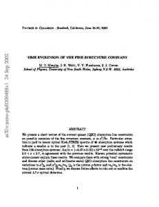
Fig. 1.— Schematic diagram of the [OIII], [NeIII], and [NeV] (left panel), and the [OII] and [SII] (right panel) line doublets

15

Fig. 2.— Optical spectra of the [NeV], [NeIII], and [OIII] regions

16

17

18

Fig. 3.— Optical spectra of the [OI] and [SII] line regions

19

Fig. 4.— Redshift vs. α2 (t)/α2 (0)

20