Sub-Domain Finite Element Method for Efficiently Considering Strong Skin and Proximity Effects Patrick Dular1, Ruth V. Sabariego1, Johan Gyselinck2, Laurent Krähenbühl3 1 University of Liège - Dept. of Electrical Engineering and Computer Science – Montefiore Inst. B28 – B-4000 Liège - Belgium 2 Université Libre de Bruxelles (ULB) – Dept. of Electrical Engineering – CP165/52 – B-1050 Brussel – Belgium 3 Université de Lyon – École Centrale de Lyon – Ampère (UMR CNRS 5005) – F-69134 Écully Cedex – France
e-mail:
[email protected]
Purpose − To develop a sub-domain perturbation technique to efficiently calculate strong skin and proximity effects in conductors within frequency and time domain finite element (FE) analyses. Design/methodology/approach − A reference eddy current FE problem is first solved by considering perfect conductors. This is done via appropriate boundary conditions on the conductors. Next the solution of the reference problem gives the source for eddy current FE perturbation sub-problems in each conductor then considered with a finite conductivity. Each of these problems requires an appropriate volume mesh of the associated conductor and its surrounding region. Findings − The skin and proximity effects in both active and passive conductors can be accurately determined in a wide frequency range, allowing for precise losses calculations in inductors as well as in external conducting pieces. Originality/value − The developed method allows to accurately determine the current density distributions and ensuing losses in conductors of any shape, not only in the frequency domain but also in the time domain. Therefore it extends the domain of validity and applicability of impedance-type boundary condition techniques. It also offers an original way to uncouple FE regions; what allows the solution process to be lightened, as well as efficient parameterized analyses on the signal form and the conductor characteristics. Keywords − Impedance boundary condition, Perturbation technique, Sub-domain finite element method, Skin and proximity effects
alternative to avoid meshing their interior. Such conditions are nevertheless generally based on analytical solutions of ideal problems and are therefore only valid in practice far from any geometrical discontinuities, e.g., edges and corners. They are also generally limited to frequency domain and linear analyses. In this contribution, a method is developed to overcome the limitations of impedance-type BCs, allowing conductors of any shape to be considered not only in the frequency domain but also in the time domain. The magnetic vector potential FE magnetodynamic formulation is used. A reference eddy current FE problem is first solved by considering perfect conductors. This can be done via appropriate conditions on the conductor boundaries, which can serve as well for expressing the circuit relations of the conductors linking their voltages and currents. Next the solution of the reference problem gives the source for eddy current FE perturbation sub-problems in each conductor considered, at this point, with a finite conductivity. Each of these problems requires an appropriate volume mesh of the associated conductor and its surrounding region. The developed technique will be validated on an application example and its domain of validity will be determined. Its main advantages versus the impedance-type boundary technique will be pointed out.
Paper type − Research paper
I. INTRODUCTION A precise consideration of the skin and proximity effects in conductors is usually important for the sources themselves as well as for their surrounding area. On the one hand, an accurate calculation of the ensuing Joule losses in the conductors themselves is possible. On the other hand, this allows to accurately locate the current density distributions with respect to the influenced regions. The skin and proximity effects are particularly significant for high frequency excitations in highly conducting materials. When such eddy current problems are solved with the classical finite element (FE) method, the ensuing small skin depth asks for a fine mesh through the conductor thickness. Impedance-type boundary conditions (BCs) (Krähenbühl and Muller, 1993) defined on the conductor boundaries are an This work was supported in part by the Belgian Science Policy (IAP P6/21) and the Belgian French Community (Research Concerted Action ARC 03/08298). P. Dular is a Research Associate with the Belgian National Fund for Scientific Research (F.N.R.S.).
II. FROM PERFECT TO NON-PERFECT CONDUCTORS – THE STRONG EDDY CURRENT FORMULATIONS A. The eddy current problem Maxwell equations are to be solved in a bounded domain Ω, with boundary ∂Ω (possibly at infinity), of the 2-D or 3-D Euclidean space. The eddy current conducting part of Ω is denoted Ωc and the non-conducting one ΩcC, with Ω = Ωc ∪ ΩcC. Massive conductors belong to Ωc. The equations and relations governing the magnetodynamic (eddy current) problem in Ω are curl h = j , curl e = – ∂t b , div b = 0 , b=μh, j=σe,
(1a-b-c) (2a-b)
where h is the magnetic field, b is the magnetic flux density, e is the electric field, j is the electric current density (including source and eddy currents), μ is the magnetic permeability and σ is the electric conductivity. In the following, the subscripts
u and p will refer to reference and perturbed quantities, respectively. B. The reference problem: some conductors are first considered as perfect Instead of directly solving the eddy current problem with the actual conductivity of some conductors, a so-called reference problem is first defined in Ω by considering some conductors Ωc, i (i is the conductor index) as being perfect, i.e. of infinite conductivity. This results in a zero skin depth and thus in surface currents. The interior of the conductor regions Ωc, i can thus be extracted from the studied domain Ω in (1) and treated via a BC fixing a zero normal magnetic flux density on their boundaries ∂Ωc, i, n ⋅ bu ∂Ω
c ,i
=0.
(3)
C. The perturbation problem: the conductors retrieve their actual conductivity The consideration of the actual conductivity of the concerned conductors, these defining the perturbing region Ωc, i ⊂ Ωc, will further lead to field perturbations. The perturbed eddy current problem focuses thus on Ωc, i and its neighborhood, their union Ωp being adequately defined and meshed will serve as the studied domain. The perturbation generated by the change of conductivity of the conducting region Ωc, i alters the distribution of the eddy current density and magnetic field. The fields in these conductors are not surface fields anymore but penetrate them. Problems with volume fields are first considered and will be further particularized for the actual reference solution with surface fields in the next section. Particularizing (1) and (2) for both the reference and perturbed quantities, and subtracting the reference equations from the perturbed ones, a perturbation problem (defined as the difference between perturbed and reference problems) is obtained in Ωp (initially in Ω) (Badics et al., 1997; Sabariego and Dular, 2005). Figs. 1 to 4 help in illustrating the involved problems. Keeping the equations in terms of the perturbations h = hp – hu and e = ep – eu, one gets in Ωp curl h = j , curl e = – ∂t b ,
(4a-b)
j = σp e + js , b = μp h + bs ,
(5a-b)
The perturbation problem (4)-(8) is rigorously defined in the whole studied domain Ω, taking account of the geometrical and material details of the reference problem. The conditions (6a) or (6b) neglect the perturbation at a certain distance from Ωc, i, which is actually only correct at infinity (for Ωp extended to the whole space). For convenience, an approximation neglecting some of these initial details will be made. The so-modified studied domain Ωp can be a portion or not of Ω, with or without inclusion of initial materials, these being possibly simplified. At the discrete level, the meshes of both reference and perturbed problems can then be significantly simplified, each problem asking for mesh refinement of different regions. D. Sources of the perturbation problem The sources js (7) and bs (8) act as sources reduced to Ωc, i. This is a consequence of the use of the perturbations h and e as unknowns instead of the perturbed fields hp and ep directly. Another implication is the homogeneous nature of the boundary conditions (6a) or (6b). The perturbed problem, with the unknown fields hp and ep, would require non-homogeneous conditions such as n × hp
∂Ω p
= n × hu
∂Ω p
or n × e p
∂Ω p
p
(6a-b)
p
where the so-defined volume sources js and bs are obtained from the reference solution as js = (σp – σu) eu in Ωc, p ,
(7)
bs = (μp – μu) hu in Ωc, p .
(8)
∂Ω p
. (9a-b)
The reference fields would thus serve as surface sources, to be projected on the mesh boundary ∂Ωp of the perturbation problem. However, such BCs can only be applied if the domain Ωp is bounded. Indeed a boundary at infinity would support a zero source, with consequently no information at all for the perturbed problem. The reference field hu could alternatively be used as a volume source field in the whole Ωp, but with the disadvantage of necessitating its evaluation and projection on the whole domain. These drawbacks justify the use of the sources js (7) and bs (8), the reduced support of which noticeably limits the evaluation and projection operations. The source bs (8), determined from the known field hu, is itself also zero in Ωc, i. The source current density js (7) is to be obtained from the reference electric field eu, with σu → ∞ and σp finite in Ωc, i. The quantities involved in (7) are, on the one hand, σu eu to be considered at the limit as a surface current density ju on ∂Ωc, i, and, on the other hand, σp eu actually being null in Ωc, i and ∂Ωc, i because eu is zero and σp is finite there. Consequently, the source current density js associated with ju has a surface nature as well js = − ju on ∂Ωc, i .
n × h ∂Ω = 0 or n × e ∂Ω = 0 ,
= n × eu
(10)
The problem (4)-(8) particularized to such a surface source can remain on its form on condition that it is written in Ωp \ ∂Ωc, i with additional relations for BCs on both sides of ∂Ωc, i (∂Ωc, i is extracted from the studied domain). This will be considered when writing its weak formulation.
III. WEAK MAGNETIC VECTOR POTENTIAL EDDY CURRENT FORMULATIONS A. b-conform weak magnetodynamic formulation The eddy current problem is defined in Ω with the magnetic vector potential formulation (Dular et al., 2000), expressing the electric field e in Ωc via a magnetic vector potential a together with the gradient of an electric scalar potential v, and the magnetic flux density b in Ω as the curl of a. The resulting a-v magnetodynamic formulation is obtained from the weak form of the Ampere equation (1a), i.e. (Dular et al., 2000), ( μ −1 curl a,curl a ')Ω + (σ ∂ t a, a ')Ωc + (σ grad v, a ')Ωc 1
+ < n × hs , a ' > Γh = 0 , ∀ a ' ∈ F (Ω) ,
(11)
B. Reference problem with perfect conductors The zero normal magnetic flux density BC on the boundaries ∂Ωc, i of the so-considered perfect conductors leads to an essential condition on the primary unknown au that can be expressed via the definition of a surface scalar potential uu (in general single valued, if no net magnetic flux flows in Ωc, i) (Dular et al., 2005), i.e., c ,i
= 0 ⇔ n × au ∂Ω
c ,i
= n × grad uu ∂Ω . c ,i
C. Perturbation eddy current problem The skin and proximity effects in each conductor Ωc, i have now to be corrected for their real conducting nature. This is done via the weak formulation of the perturbation problem (4)-(8), i.e. ( μ p −1 curl a, curl a ')Ω p + (σ p ∂ t a, a ')Ωc \Ωc ,i + (σ p grad v, a ')Ωc \Ωc ,i + (σ p ∂ t a, a ')Ωc ,i + (σ p grad v, a ')Ωc ,i
where F1(Ω) is a gauged curl-conform function space defined on Ω and containing the basis functions for a as well as for the test function a' (at the discrete level, this space is defined by edge finite elements); ( · , · )Ω and < · , · >Γ respectively denote a volume integral in Ω and a surface integral on Γ of the product of their vector field arguments. The surface integral term in (11) accounts for the natural boundary or interface conditions. It will be shown to be of key importance in our further developments.
n ⋅ curl au ∂Ω
∂Ωc, i). This way, the circuit relation can be expressed for each conductor Ωc, i and the coupling with electrical circuits is possible. The other surface integral on Γh is used for classical natural BCs.
(12)
In a 2D model, with perpendicular currents, condition (12) amounts to define a floating (constant) value for the perpendicular component of au for each conductor. The reference formulation is of the form (11) with all the quantities with the subscript u, i.e. ( μu −1 curl au , curl a ')Ω + (σ u ∂t au , a ')Ωc \ Ωc ,i + (σ u grad vu , a ')Ωc \ Ωc ,i + < n × hu , a ' >∂Ωc ,i + < n × hs ,u , a ' >Γ h = 0, ∀ a ' ∈ Fu1 (Ω). (13)
The conductors considered as perfect are separated from the other classical conductors (Ωc \ Ωc, i) and are only involved through their boundaries ∂Ωc, i in (13) with the condition (12). The surface integral term on ∂Ωc, i is non-zero only for the function grad ui' (from (12) for conductor i), the value of which is then the total current I i flowing through ∂Ωc, i (this can be demonstrated from the general procedure developed in Dular et al. (2000)). It is zero for all the other local test functions (at the discrete level, for any edge not belonging to
+ < n × hu , a ' >∂Ωc ,i = 0, ∀ a ' ∈ F 1 (Ω).
(14)
Note that the perturbation eddy current density in Ωc \ Ωc, i (in which σp = σu) can be neglected, in which case the second and third terms in (14) can be omitted. The surface integral term related to ∂Ωc, i in the perturbation formulation (14) is actually known from the reference solution. The surface ∂Ωc, i is now considered as a part of the studied domain with contributions on both sides, i.e. in Ωc, i and Ωp \ Ωc, i. This surface term is determined as follows. The quantity n × hu in (14), directly linked to the tangential reference magnetic field, acts as the surface current density ju involved in (10). It is not known in a strong sense on ∂Ωc, i, but rather in a weak sense via the surface term in (13); this is a consequence of the b-conform formulation used. This same surface term is also implied in (14) and will thus be expressed via the reference solution fixed in (13), i.e. < n × hu , a ' >∂Ωc ,i = − ( μu −1 curl au , curl a ')Ω ,
(15)
in case no part of Ωc \ Ωc, i is in contact with Ωc, i (otherwise the second and third terms of (13) have to be considered as well). This way, the surface source current density js to be used in the perturbation weak formulation is then calculated from a volume integral coming from the reference problem. Its consideration via a volume integral, limited at the discrete level to one single layer of FEs touching the boundary, is the natural way to average it as a weak quantity. At the discrete level, the source quantity js initially given in the mesh of the reference problem has to be expressed in the mesh of the perturbation problem. This can be done through a projection method (Geuzaine et al., 1999) with target quantity js defined in adequate function spaces. From (4a) and (5a), the projected js should have the same conformity as curl h. The source quantity js can then be used in (14), the solution of which gives the eddy current density in Ωc, i and the ensuing field perturbations in and outside Ωc, i. IV. APPLICATION A core-inductor system is considered as a test problem (Fig. 1). The three copper stranded inductor portions (conductivity σCu = 5.9 107 Ω–1m–1) have a square section (width
12.5 mm) and are connected in series. The core is made of aluminium (conductivity σAl = 2.7 107 Ω–1m–1). A 2D model with a vertical symmetry axis is considered. For a direct comparison with the technique using impedance-type BCs, a frequency domain analysis is done. However, the sub-domain perturbation technique can be directly applied to time domain analyses without any change. The working frequency is 5 kHz (skin depth δAl in aluminium of 1.37 mm). The core has a half-width of 12.5 mm (9.1 δAl) and a length of 50 mm (36.5 δAl). The results focus on the aluminium core. Holes in the core are considered in order to point out the effect of several corners. These holes are non-uniformly distributed to allow for different lengths of plane portions between them (small lengths should penalize the impedance BC technique). The different meshes used, the magnetic flux lines and the magnetic flux density distributions (zoomed or not) are shown respectively in Figs. 1 to 4 for the different calculations performed, i.e. the conventional FE approach (used as a reference), the reference problem and the perturbation problem. Figs. 5 to 7 concern the eddy current and Joule power density distributions in the core. It can be seen that the perturbation method determines the perturbation fields with a very good accuracy, as well for the magnetic flux density as for the eddy current density. In particular, the correction of the magnetic flux density in the vicinity of the corners (Figs. 3 and 4, right) leads to its actual distribution in the core (along the skin depth) and to the reduction of the over-evaluated reference value in the exterior region (Fig. 4, see the opposite direction of the magnetic flux density ). Fig. 7 highlights the relative error on the current density (from Fig. 6) and the associated Joule power density made by the impedance BC technique versus the sub-domain FE approach (the results of which have been checked to be very similar to those given by the conventional FE approach). The error significantly increases in the vicinity of the conductor corners: it exceeds 50% for the Joule power density and 30% for the current density in the smallest plane portions. This affects the total losses accuracy when the size of the conductor portions decreases. The error with the impedance BC technique is shown to be significant up to a distance of about 3 δAl from each corner, whereas a good accuracy is only obtained beyond this distance. V. CONCLUSIONS The developed sub-domain perturbation method offers a way to uncouple FE regions in eddy current frequency and time domain analyses with high frequency excitations, allowing the solution process to be lightened. The skin and proximity effects in both active and passive conductors can be accurately determined in a wide frequency range, allowing precise losses calculations in inductors as well as in external conducting pieces, in particular in inductively heated pieces. Once calculated, the source reference solution can be used in each sub-problem not only for a single high frequency signal but for several signals. This allows efficient parameterized analyses on the signal form and the electric and magnetic characteristics of the conductors in a wide range, i.e. on all
the parameters affecting the skin depth. Nonlinear analyses, e.g. with temperature dependent conductivities, could then clearly benefit from this.
Fig. 1. Meshes for the conventional FE approach (left), the reference problem (middle) and the perturbation problem (right).
Fig. 2. Magnetic flux lines for the conventional FE solution (left), the reference solution (middle) and the perturbation solution (right).
Fig. 3. Magnetic flux density for the conventional FE solution (left), the reference solution (middle) and the perturbation solution (right).
Relative error with impedance BC (%)
60
50
40
30
20
10
0 -25
Fig. 4. Magnetic flux density (zoom in the upper corner of the core) for the classical FE solution (left), the reference solution (middle) and the perturbation solution (right).
Joule power density Current density
-20
-15
-10 -5 0 5 10 Position along core surface (mm)
15
20
25
Fig. 7. Relative error on the current density and the associated Joule power density along the core surface made by the impedance BC technique versus the sub-domain FE approach.
REFERENCES
Fig. 5. Eddy current density distribution for the perturbation solution (left: phase 180°, right: modulus). 0.55
Conventional FEM Perturbation technique (finite ext. region) Perturbation technique (infinite ext. region) Impedance BC
2
Current density (A/mm )
0.5 0.45 0.4 0.35 0.3 0.25 0.2 -25
-20
-15
-10 -5 0 5 10 Position along core surface (mm)
15
20
25
Fig. 6. Eddy current density along the core surface for the conventional FE solution, the perturbation technique and the impedance BC technique.
Badics, Z. et al. (1997), “An effective 3-D finite element scheme for computing electromagnetic field distortions due to defects in eddycurrent nondestructive evaluation”, IEEE Trans. Magn., Vol. 33 No. 2, pp. 1012-20. Dular, P., Gyselinck, J., Henneron, T. and Piriou, F. (2005), “Dual finite element formulations for lumped reluctances coupling”, IEEE Trans. Magn., Vol. 41 No. 5, pp. 1396-9. Dular, P., Kuo-Peng, P. , Geuzaine, C., Sadowski, N. and Bastos, J.P.A. (2000), “Dual magnetodynamic formulations and their source fields associated with massive and stranded inductors”, IEEE Trans. Magn., Vol. 36 No. 4, pp. 3078-81. Geuzaine, C., Meys, B., Henrotte, F., Dular, P. and Legros, W. (1999), “A Galerkin projection method for mixed finite elements”, IEEE Trans. Magn., Vol. 35 No. 3, pp. 1438-41. Krähenbühl, L. and Muller, D. (1993), “Thin layers in electrical engineering. Example of shell models in analyzing eddy-currents by boundary and finite element methods”, IEEE Trans. Magn., Vol. 29, No. 2, pp. 14501455. Sabariego, R. V. and Dular, P. (2005), “A perturbation technique for the finite element modelling of nondestructive eddy current testing”, in Proc. International Symposium on Electromagnetic Fields in Mechatronics, Electrical and Electronic Engineering (ISEF), Sept. 1517, CD-ROM, paper CE-2.5, 7 pages.


![[hal-00612473, v1] A mixed finite element method for ...](https://m.moam.info/img/260x300/hal-00612473-v1-a-mixed-finite-element-method-for-_5ba02924097c47277e8b45c9.jpg)