Subband Encoding of High Dynamic Range Imagery - CiteSeerX

Subband Encoding of High Dynamic Range Imagery Greg Ward Sunnybrook Technologies

Abstract The transition from traditional 24-bit RGB to high dynamic range (HDR) images is hindered by excessively large file formats with no backwards compatibility. In this paper, we propose a simple approach to HDR encoding that parallels the evolution of color television from its grayscale beginnings. A tone-mapped version of each HDR original is accompanied by restorative information carried in a subband of a standard 24-bit RGB format. This subband contains a compressed ratio image, which when multiplied by the tone-mapped foreground, recovers the HDR original. The tone-mapped image data may be compressed, permitting the composite to be delivered in a standard JPEG wrapper. To naïve software, the image looks like any other, and displays as a tone-mapped version of the original. To HDRenabled software, the foreground image is merely a tone-mapping suggestion, as the original pixel data are available by decoding the information in the subband. We present specifics of the method and the results of encoding a series of synthetic and natural HDR images, using various published global and local tone-mapping operators to generate the foreground images. Errors are visible in only a very small percentage of the pixels after decoding, and the technique requires only a modest amount of additional space for the subband data, independent of image size. CR Categories: I.3.3 [Computer Graphics]: Picture/Image generation – Display Algorithms I.4 [Image Processing and Computer Vision]: I.4.10 Image Representation Keywords: high dynamic range image formats, lossy compression, image processing

1. Introduction Visible light in the real world covers a vast dynamic range. Humans are capable of simultaneously perceiving over 4 orders of magnitude (1:10000 contrast ratio), and can adapt their sensitivity up and down another 6 orders. Conventional digital images, such as 24-bit sRGB [Stokes et al. 1996], hold less than 2 useful orders of magnitude. Such formats are called “output-referred” standards because they are tailored to what can be displayed on a common CRT monitor – colors outside this limited gamut are not represented. A “scene-referred” standard is designed instead to represent colors and intensities that are visible in the real world, and though they may not be rendered faithfully on today’s output devices, they will be visible on displays in the near future [Seetzen et al. 2003]. Such image representations are referred to as extended gamut or high dynamic range (HDR) formats, and a few alternatives have been introduced over the past 15 years, mostly by the graphics research and special effects communities.

Maryann Simmons Walt Disney Feature Animation

Unfortunately, none of the existing or proposed HDR formats supports lossy compression, and only one comes in a conventional image wrapper. These formats yield prohibitively large images that can only be viewed and manipulated by specialized software. Commercial hardware and software developers have been slow to embrace scene-referred standards due to their demands on image capture, storage, and use. Some digital camera manufacturers attempt to address the desire for greater exposure control during processing with their own proprietary RAW formats, but these camera-specific encodings fail in terms of image archiving and third-party support. They are convenient for the manufacturers, but for no one else. What we really need is a compact image that looks and displays like an output-referred JPEG, but holds the extra information needed to enable it as a scene-referred standard. Future HDR cameras will then be able to write to this format without fear that the software on the receiving end won’t know what to do with it. Conventional image manipulation and display software will see only the tone-mapped version of the image, gaining some benefit from the HDR capture due to its better exposure. HDR-enabled software will have full access to the original dynamic range recorded by the camera, permitting large exposure shifts and contrast manipulation during image editing. Establishing such a standard will provide a smooth upgrade path for manufacturers and consumers alike.

1.1.

Background

High dynamic range imaging goes back many years. A few early researchers in image processing advocated the use of logarithmic encodings of intensity (e.g., [Jourlin & Pinoli 1988]), though it was global illumination that brought us the first standard. A space-efficient format for HDR images was introduced in 1989 as part of the Radiance rendering system [Ward 1991; Ward 1994]. However, the Radiance RGBE format was not widely used until HDR photography and environment mapping were developed by Debevec [Debevec & Malik 1997; Debevec 1998]. About the same time, Ward Larson [1998] introduced the LogLuv alternative to RGBE and distributed it as part of Leffler’s public TIFF library [Leffler et al. 1999]. The LogLuv format has the advantage of covering the full visible gamut in a more compact representation, whereas RGBE is restricted to positive primary values. A few graphics researchers adopted the LogLuv format, but most continued to use RGBE (or its extended gamut variant XYZE), until Industrial Light and Magic made their EXR format available in 2002 [Kainz et al. 2002]. The OpenEXR library uses the same basic 16-bit floating point data type as modern graphics cards, and is poised to be the new favorite in the special effects industry. Other standards have also been proposed or are in the works, but they all have limited dynamic range relative to their size (e.g., [IEC 2003]). None of these standards is backwards compatible with existing software. The current state of affairs in HDR imaging parallels the development of color television after the adoption of black and white broadcast. A large installed base must be accommodated as

2 well as an existing standard for transmission. The NTSC solution introduced a subband to the signal that encoded the additional chroma information without interfering with the original black and white signal [Jolliffe 1950]. We propose a similar solution in the context of HDR imagery, with similar benefits. As in the case of black and white television, we have an existing, de facto standard for digital images: output-referred JPEG. JPEG has a number of advantages that are difficult to beat. The standard is unambiguous and universally supported. Software libraries are free and widely available. Encoding and decoding is fast and efficient, and display is straightforward. Compression performance for average quality images is competitive with more recent advances, and every digital camera writes to this format. Clearly, we will be living with JPEG images for many years to come. Our chances of large scale adoption increase dramatically if we can maintain backward compatibility with this standard. Our general approach is to introduce a subband that accompanies a tone-mapped version of the original HDR image. This subband is compressed to fit in a metadata tag that will be ignored by naïve applications, but can be used to extract the HDR original in enabled software. We utilize JPEG/JFIF as our standard wrapper in this implementation, but our technique is compatible with any format that provides client-defined tags (e.g., TIFF, PNG, etc.). The Method section of our paper describes the basic idea behind HDR subband encoding, followed by a more detailed description of the steps involved and our trial implementation. The Results and Discussion section presents a set of example images and examines sources of error in our encoding. We end with our conclusions and future directions.

Encoder (÷)

24-bit TM´

Compress & Format

Subband RI TMO

24-bit TM

Conventional Decompress

Standard Compressed Image with Subband

Decompress w/ Subband

24-bit TM´d

24-bit TM´d

Decoder (
)

Subband RId

Recovered HDRd

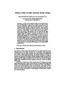
Figure 2. Alternate decoding paths for compressed composite. Figure
2 shows the two possible decoding paths. The high road decompresses both the tone-mapped foreground image and the subband, delivering them to the decoder to recover the HDR pixels. Naïve applications follow the low road, ignoring the subband in the metadata and reproducing only the tone-mapped foreground image. In the simplest incarnation of this method, the encoder divides the HDR pixels by the tone-mapped luminances, producing an 8-bit ratio image that is stored as metadata in a standard JPEG compressed image. Decoding follows decompression with a multiplication step to recover the original HDR pixels. Unfortunately, the simplest approach fails for pixels that are mapped to black or white by the tone-mapping operator (TMO), and the limited size of metadata in JPEG makes subband compression a challenge. These are two important issues we must address with our technique.

2.1.

2. Method Original HDR

Standard Compressed Image with Subband

The Ratio Image

JPEG/JFIF offers us a limited subband channel, called the “application markers.” Sixteen application markers exist in the JFIF specification, three of which are spoken for. A marker may hold up to 64 Kbytes of data, regardless of the image dimensions. This is an important limitation in our method – we want to keep our subband data under 64K, independent of image size. The foreground signal in our application is a tone-mapped version of the original HDR image. This output-referred image is stored in the usual 8
8, 8-bit blocks using JPEG’s lossy DCT compression [Wallace 1991]. The subband encodes the information needed to restore the HDR original from this compressed version. Let us assume that our selected tone-mapping operator possesses the following properties:

Figure 1. High level HDR subband encoding pipeline. Figure
1 shows an overview of our HDR encoding pipeline. We start with two versions of our image: a scene-referred HDR image, and an output-referred, tone-mapped version. If we like, we can generate this tone-mapped version ourselves, but in general this is a separable problem, because our technique is designed to work with multiple operators. The encoding stage takes these two inputs and produces a composite, consisting of a potentially modified version of the original tone-mapped image, and a subband ratio image that contains enough information to reproduce a close facsimile of the HDR original. The next stage compresses this information, offering the tone-mapped version as the JPEG base image, and storing the subband as metadata in a standard JFIF wrapper.

A.

The original HDR input is mapped smoothly into a 24-bit output domain, with no components being rudely clamped at 0 or 255.

B.

Hue is maintained at each pixel, and mild saturation changes can be described by an invertible function of input and output value.

Most tone-mapping operators for HDR images have the first property as their goal, so this should not be a problem. If it is, we can override the operator by locally replacing each clamped pixel with a lighter or darker value that fits the range. Similarly, we can enforce the second property by performing our own color desaturation, using the tone-mapping operator as a guide only for

3 luminance changes. Most tone-mapping operators address color in a very simple way, if they consider it at all.1 Exceptions are found in operators that simulate human vision (e.g., [Pattanaik et al. 1998]), whose support we leave as future work. Given these restrictions, a ratio image may be computed by dividing the HDR original luminance at each pixel by the tonemapped output luminance:

RI(x, y) =

L(HDR(x, y)) L(TM(x, y))

(1)

The ratio image is compressed and sent in our subband along with the saturation formula. The tone-mapped version is then encoded as the foreground image, modified as necessary to avoid clamping. During reconstruction, the ratio image is multiplied by the foreground image to recover the original HDR luminance values. Color is then restored using the recorded saturation formula. (See Appendix for details.)

2.2.

Figure 3. Memorial Church shown tone-mapped with Reinhard's global operator (left) along with the log-encoded ratio image needed for HDR recovery (right).3

Subband Compression

Obviously, we will not meet our goal of fitting the subband into 64 Kbytes if we send the ratio image along uncompressed. Since our goal is to encapsulate the subband in a JPEG wrapper, it would be most convenient if we could compress the ratio image using JPEG as well.2 If we could also fix the maximum size of the ratio image, we could avoid the problem of needing more space or greater compression for larger input images. Figure
3 shows the Memorial Church image, tone-mapped using the global zone operator of Reinhard et al. [2002]. Ratio values are mapped into an 8-bit range by a log encoding that captures the extrema, as we show on the right. Because the original image is only 512x768 pixels, we can compress our ratio image into 48 Kbytes with a JPEG quality setting of 90, without resorting to downsampling. We see a before and after close-up of the recovered HDR image near the window, where luminance compression is greatest, in Figure
4. A comparison of the dark ceiling is shown on the left. Qualitatively, we are able to reproduce the original HDR pixels using this method, although JPEG artifacts are beginning to appear. Clearly, we cannot push this approach to much larger images and hope to stay within the 64 Kbyte limit. Figure
5 shows a 2048x1536 image of the Dyrham Church next to its reduced ratio image. In this composite, we have downsampled the subband image to 768x576 and compressed it to 41 Kbytes using the same JPEG quality setting of 90. Recovery is quite good in darker regions, as shown on the right of Figure
6, but we start to lose focus on bright boundaries, such as the window panes shown on the left. This is due to blur in the ratio image introduced when we upsample prior to multiplication. We need some method of recovering the high frequencies we lost when we downsampled the ratio image. In the following sections, we present two alternate recovery methods: precorrecting the foreground image, and postcorrecting the ratio image.

Figure 4. Linear displays of original (top) and recovered (bottom) HDR images. On the left is a close-up of the ceiling, and on the right is a close-up of the rightmost windows.3

Figure 5. The Dyrham Church image rendered with Reinhard’s global operator, shown next to the corresponding downsampled ratio image.

1

We can use a fitting function to match desaturation of the exemplar tonemapped image if it is unknown. 2 The Exif files produced by digital cameras use this trick for storing thumbnail images.

3

Figures 3, 4, 6, 7, 8, 9, 10, 12, and 13 are repeated on the color plate.

4

Figure 6. Details of the image recovered using the downsampled subband.3

2.3.

Precorrection of Foreground Image

2.4.

One way to retain the high frequency information is to precorrect the foreground image based on the compressed subband. After computing the subband as above, we redivide the HDR original by the decompressed and upsampled ratio image to get a modified foreground image:

TM
=

HDR RId

Figure 8. Linear comparison of HDR image recovery improved by precorrecting the tone-mapped foreground image.3

(2)

Substituting this modified foreground image for the original effectively undoes the damage of lossy compression and downsampling. The left image in Figure
7 shows the lattice window after applying Reinhard’s global tone-mapping operator to the Dyrham Church image. On the right, we see the result of dividing the HDR original by the computed ratio image. By construction, the result of multiplying this modified foreground image by our downsampled ratio image will be very close to the original, even after JPEG transmission. Figure
8 shows a linear rendition of the HDR original next to the recovered result. The precorrection method is a good complement to Reinhard’s operator because it restores some of the contrast lost at the high end. However, the sharpening produced by this technique may be undesirable when the TMO has already produced an optimal foreground image. In such cases, we may prefer not to modify the foreground image during encoding, choosing instead to recover high frequencies in a post-process.

Postcorrection of Ratio Image

If we invest the time to generate a high quality foreground image with a sophisticated TMO, we may be unwilling to accept the effects of precorrection as described in the previous section. For a sufficiently high resolution original, recomputing TM´ using Eq.
(2) can result in small halos that are visible in close-ups, as shown in the sunset of Figure
9.

Figure 9. Reverse gradients visible on a modified high-resolution (3000x1700) foreground image. The original bilateral filter tonemapping is shown on the left inset.3 Ideally, we would like to preserve the tone-mapped representation in the foreground image without losing resolution in the recovered HDR result. One way to achieve this without exceeding our 64 Kbyte subband limit is to synthesize the missing high frequencies in our resampled ratio image. Since we have a full-resolution foreground image, we can use this as a guide for where edges belong in the ratio image. If the frequency content of the foreground image and the ratio image before downsampling were the same, one could recover the high frequencies in the resampled ratio image with the following simple formula:

RIsynth = RId

Figure 7. Reinhard’s tone-mapping operator applied to the Dyrham Church image, before and after modification by the downsampled ratio image in our precorrection method.3

L(TM) L(TM r )

In this equation, L(TMr) is the luminance of the tone-mapped foreground image, resampled in the same way as the encoded ratio image. Of course, there is no guarantee that the frequency content of the foreground and ratio images are the same, especially using a TMO like the bilateral filter, which attempts to

5 preserve local detail [Durand & Dorsey 2002]. A better approximation therefore attenuates the effect by the ratio between the local variance of RId and TMr. If the ratio image has little or no variance after resampling, then it probably had little in the way of high frequencies beforehand. This improved frequency correction may be written as follows:


 L(TM)  RIsynth = RId     L(TM r )  var(RId ) where :
= var(L(TM r ))

(3)

The relative variance is computed over a small neighborhood, equal to the resampling radius, and  is set to 0 if var(L(TMr)) is less than our compression-decompression error. In practice, we do not allow the exponent  to exceed 1, as this can cause overshooting in the output. We define relative variance as the difference between the maximum and minimum in a neighborhood, divided by the central value. This is a simple application of resolution enhancement via example learning. Much more sophisticated techniques have been developed by the vision community [Baker & Kanade 2002]. Figure
10 shows the results of applying high frequency synthesis to the Napa Valley image. The foreground image for this encoding was computed using a bilateral filter, hence there are significant discrepancies between the tone-mapped version and the ratio image. As we can see, the approximation in Eq.
(3) does a reasonable job of restoring the high frequency information that has been lost during the resampling process, without introducing objectionable artifacts. However, the errors in the recovered HDR image are greater with this method than those of Eq.
(2), so the application should decide whether the benefits of a cleaner foreground image are worth the costs. A flag must be passed in the subband, indicating whether the image was precorrected by Eq.
(2), or should be postcorrected by Eq.
(3). Figure 11. Test image set.

Figure 10. The center is the original HDR image with a linear tone-mapping. On the left is our uncorrected ratio image multiplied by the foreground image. On the right, we postcorrected the ratio image with synthetic high frequencies.3

3. Results and Discussion We tested our encoding on the fifteen HDR images shown in Figure
11. Table
1 lists each image size and dynamic range in base 10 units. (E.g., 4.8 is 1:104.8 or 1:63,000 dynamic range.)

Image

Size

Bathroom Dani_belgium Dani_cathedral Desk DyrhamChurch FogMap Hotel MtTamWest Memorial NapaValley PriceWestern SGcover92 TimesSquare Tree Tunnel

346
512 1025
769 767
1023 644
874 2048
1536 751
1130 3000
1950 1214
732 512
768 3025
2129 3272
1280 1024
1024 2272
1704 928
906 5462
4436

Dynamic Range 4.8 5.8 4.8 5.2 4.0 4.1 4.7 4.1 5.5 5.3 3.7 4.7 3.6 4.1 9.2

Source Radiance digital digital film digital film Radiance film film Spheron Spheron Radiance digital film Radiance

Table 1. Test image sizes. Images were either synthetic (Radiance renderings), or captured (multiple film or digital exposures, or panoramic SpheronVR scans). Eleven images are captures of natural scenes, and four are synthetic. The dynamic ranges of the images are between 3.6 and 9.2 orders of magnitude, with 4.9 being average. The smallest

6 image is 346512; the largest is 54624436, and the median is 0.9 megapixels. We tested four different tone-mapping operators to produce the foreground image: Ward Larson et al.’s histogram method [1997], Reinhard et al.’s global zone method [2002], Fattal et al.’s gradient operator [2002], and Durand & Dorsey’s bilateral filter method [2002]. Our test procedure was simple: encode then decode each image using the selected TMO and JPEG compression parameters, then compare the recovered HDR image to the original. We tested two JPEG compression levels (quality settings) on the foreground image: 90 and 100, using Tom Lane’s public JPEG implementation. The ratio image was always compressed with the highest JPEG quality setting that kept the result under 60 Kbytes, leaving ample room for other subband data. If the original image was greater than 400,000 pixels, the ratio image was downsampled to this size before compression.

region of this image, verifying the correlation between actual perceptible differences and VDP on the arm of the chair. Empirically, we found VDP to be an excellent predictor of where we could see differences in our images. Our results are summarized in Table
2, where we have averaged the VDP percentages over all images except “Tunnel,” which we considered an outlier. We see a sizeable discrepancy in the VDP results for different tone-mapping operators, and for precorrection versus postcorrection. The JPEG quality setting also made a difference, as one would expect. TMO Bilateral Filter Reinhard Global Histogram Adj. Gradient

Quality 90 100 90 100 90 100 90 100

VDP (pre) 0.93% 0.02% 2.5% 0.09% 5.9% 0.63% 7.5% 3.0%

VDP (post) 5.4% 1.8% 4.7% 2.8% 21% 17% 36% 34%

Table 2. Percentage of perceptibly different pixels summed over all images for four tone mapping operators using VDP metric on precorrected and postcorrected encodings. Two JPEG quality settings were tested for each foreground image. Image Bathroom Dani_belgium Dani_cathedral Desk Figure 12. Sample VDP output for Hotel image. Red shows threshold where difference detection probability exceeds 0.75.3 (Green p
0.5, Yellow p
0.63, Purple p > 0.95)

DyrhamChurch FogMap Hotel Memorial MtTamWest NapaValley PriceWestern SGcover92

Figure 13. Close-up of Hotel chair’s arm from box in Figure
12 with VDP visualization.3 To compare our decoded HDR images to their corresponding originals, we employed Daly’s Visible Differences Predictor (VDP) [1993]. This metric tells us what percentage of our decoded image pixels are likely (probability p > 0.75) to be perceived as different from the originals under standard viewing conditions. Figure
12 visualizes the VDP output for the postcorrected Hotel encoding using the bilateral filter with JPEG quality set to 100. Figure
13 shows a close-up of the indicated

TimesSquare Tree Tunnel

Qual. 90 100 90 100 90 100 90 100 90 100 90 100 90 100 90 100 90 100 90 100 90 100 90 100 90 100 90 100 90 100

CR 9.6 5.7 14.4 5.3 12.3 4.5 10.7 4.6 21.3 6.4 16.6 5.9 26.0 7.9 10.3 4.4 14.2 4.9 26.3 6.9 14.5 5.0 18.3 6.2 22.4 6.7 9.6 3.9 23.5 7.3

VDP (pre) 1.3% 0.00% 0.32% 0.01% 0.24% 0.00% 0.06% 0.02% 0.03% 0.00% 0.90% 0.00% 0.14% 0.04% 5.3% 0.01% 2.4% 0.00% 0.01% 0.01% 2.1% 0.16% 0.01% 0.00% 0.08% 0.01% 0.09% 0.00% 5.3% 3.0%

VDP (post) 0.00% 0.00% 6.2% 3.0% 2.7% 1.1% 2.7% 1.8% 3.2% 1.5% 1.2% 0.22% 7.1% 2.8% 12.3% 0.76% 4.5% 0.17% 1.9% 1.6% 27.3% 9.8% 0.50% 0.47% 4.0% 1.4% 1.9% 0.42% 53% 45%

Table 3. Compression ratios and VDP percentages for each of the test images, mapped with the bilateral filter TMO.

7 The bilateral filter proved to be an excellent fit to our encoding scheme, with lower associated errors than the other techniques. The Reinhard TMO also fared reasonably well, but the histogram and gradient methods generated many visible errors, especially when coupled with our postcorrection method. Most of these errors occurred in darker regions, where pixels were mapped to very small values. This is not a general indictment of these operators – it simply means they are less suited for splitting information between foreground and ratio images as our method requires. Our results using the bilateral filter are broken out for each image in Table
3. When using a precorrected foreground image with low JPEG compression, only the Tunnel image had more than a small percentage of pixels where differences were discernable. These percentages got larger for the lower quality setting, reaching 5.3% for the Memorial image, but remained acceptable for most of the others. (We found 2% to be a reasonable cut-off for a good sideby-side match.) In all but a few cases, the postcorrected results were acceptable with the higher JPEG quality, but VDP reached a few percent for about half our images on the lower setting, and showed a real failure on the Tunnel image. We measured our compression performance relative to an uncompressed RGBE original (i.e., 32 bits/pixel). The compression ratios varied so little between precorrected and postcorrected encodings that we averaged the two in Table
3. At a foreground quality setting of 90, we saw compression ratios between 9.6 and 26.3, with an average performance of 17.0. Taking a typical example, the Fog Map image compressed from its original 3.2 Mbytes down to 200 Kbytes. At a foreground quality setting of 100, we saw compression ratios ranging from 3.9 to 7.9, with an average performance of 5.7. Unsurprisingly, the smallest compression ratios were associated with the smallest original images. The highest compression ratios were associated with the Napa Valley image. For comparison, the average compression ratio achieved by the most sophisticated, lossless HDR image format is 1.6 on this data set, using OpenEXR’s “PIZ” wavelet encoding [Kains et al. 2002].

We would expect our errors to increase somewhat for larger images with higher dynamic range, since the ratio image must be scaled to fit both these input parameters. Examining our bilateral filter results, we searched for correlations between VDP and image size, and VDP and dynamic range, but found no significant trends in our data, with the exception of a single outlier: the Tunnel. This is really the worst case image for our algorithm – not only is it the largest (23 Mpixel), it also has the greatest dynamic range (a billion to 1), and since it came unfiltered out of a stochastic ray-tracing program, it contains abnormal amounts of high frequency, HDR pixel noise. Our postcorrection algorithm had visible errors over half the image, and even precorrection could not cope where sampling discontinuities exceeded the 8-bit carrying capacity of the foreground image. For example, Figure
14 shows a halo around the sun that derives from a huge luminance discontinuity – almost 5 orders of magnitude between neighboring pixels. This is an extreme jump that could only be generated synthetically, and demands an encoding that carries 16 bits at every pixel. Therefore, we may wish to consider ways to bypass the restriction on the ratio image resolution for such extreme images, possibly working around the 64 Kbyte limit for JPEG markers by stringing multiple markers in series, which is permitted by the JFIF standard.

4. Conclusion and Future Directions By providing a lossy, high dynamic range image format that is backwards compatible with existing JPEG software, we remove an important barrier to the adoption of HDR imaging technology by digital camera manufacturers and web content providers. The subband encoding method we presented couples a high quality, tone-mapped (i.e., output-referred) foreground image with metadata that enables HDR software to recover the original, scene-referred luminances at 16-bit resolution. Naïve applications see only the tone-mapped version, which still encompasses the larger dynamic range, albeit with 8-bit precision. Color is encoded in the foreground image as well, which HDR-enabled applications may resaturate to access a wider gamut than standard RGB. With the current prototype implementation, we obtain predicted visible differences at only a very small percentage of the pixels over a wide range of HDR image sizes, adding just 64 Kbytes of subband data to each tone-mapped JPEG. Although it will not affect the critical standardization of the subband format and decoding method, there is more work to do in finding an optimal tone-mapping operator for the encoding. We found Durand and Dorsey’s bilateral filter [2002] to behave quite well, and Reinhard et al.’s global operator [2002] to perform adequately, but further testing is needed. We would like to incorporate an operator that is fast, robust, and completely automatic. Further, we would like to explore tuning of this operator to minimize problems in the ratio image that could show up as artifacts in the decoded HDR result.

Figure 14. Close-up showing details lost in small regions of the Tunnel due to downsampling of the ratio image.

Although our initial implementation is tied to the standard JPEG encoding, there is no reason the same separation of tone-mapped and ratio image could not be applied within other existing and emerging image standards. The advantage to this approach over a direct extension to incorporate an HDR color space is two-fold. Firstly, an output-referred image is immediately available to all applications, avoiding the need for a potentially time-consuming tone-mapping step prior to viewing. Secondly, separate control is possible for the fidelity/bitrate of the output-referred and scenereferred versions, permitting application-tuned encodings. As an

8 added benefit, web-savvy formats such as PNG and JPEG 2000 can send the ratio image as a separate bundle only when requested by the client, eliminating the associated cost of this additional information where it is not needed. In other words, there may be benefits to backwards compatibility looking forward as well.

The VDP implementation was provided by Karol Myszkowski, and Dave Shreiner helped process all the data. Thanks to Paul Debevec, Dani Lischinski, Erik Reinhard, Jack Tumblin, Spheron Corporation, and ILM for lending their HDR images. Thanks also to Scott Daly for useful insights into his VDP metric.

TUMBLIN, J., and TURK, G. 1999. LCIS: A Boundary Hierarchy for Detail-Preserving Contrast Reduction. ACM Trans. on Graphics, 21, 3, 83-90. WALLACE, G. 1991. The JPEG Still Picture Compression Standard. Communications of the ACM, 34, 4, 30-44. WARD LARSON, G., RUSHMEIER, H., and PIATKO, C. 1997. A Visibility Matching Tone Reproduction Operator for High Dynamic Range Scenes. IEEE Trans. on Visualization and Computer Graphics, 3, 4. WARD LARSON, G. 1998. Overcoming Gamut and Dynamic Range Limitations in Digital Images. Proc. of IS&T 6th Color Imaging Conf. WARD, G. 1991. Real Pixels. In Graphics Gems II, edited by James Arvo, Academic Press, 80-83. WARD, G. 1994. The RADIANCE Lighting Simulation and Rendering System. , In Proceedings of ACM SIGGRAPH 1994, 459-472.

6. References

7. Appendix: Color Saturation and Gamut

5. Acknowledgements

ASHIKHMIN, M. 2002. A Tone Mapping Algorithm for High Contrast Images. In Proceedings of 13th Eurographics Workshop on Rendering, 145-156. BAKER, S & KANADE, T. 2002. Limits on super-resolution and how to break them. IEEE Transactions on Pattern Analysis and Machine Intelligence., 24(9):1167-1183, September. 2002. CHIU, K. HERF, M., SHIRLEY, P., SWAMY, M., WANG, C., and ZIMMERMAN, K., 2002. A Tone Mapping Algorithm for High Contrast Images. In Proceedings of 13th Eurographics Workshop on Rendering, 245-253. DALY, S. 1993. The Visible Differences Predictor: An Algorithm for the Assessment of Image Fidelity. In Digital Images and Human Vision, A.B. Watson, editor, MIT Press, Cambridge, Massachusetts. DEBEVEC, P., and MALIK, J. 1997. Recovering High Dynamic Range Radiance Maps from Photographs. In Proceedings of ACM SIGGRAPH 1997, 369-378. DEBEVEC, P. 1998. Rendering Synthetic Objects into Real Scenes: Bridging Traditional and Image-Based Graphics with Global Illumination and High Dynamic Range Photography. In Proceedings of ACM SIGGRAPH 1998, 189-198. DURAND, F., and DORSEY, J. 2002. Fast Bilateral Filtering for the Display of High-Dynamic Range Images. ACM Transactions on Graphics, 21, 3, 249-256. FATTAL, R., LISCHINSKI, D., and WERMAN, M. 2002. Gradient Domain High Dynamic Range Compression. ACM Transactions on Graphics, 21, 3, 257-266. IEC. 2003. 61966-2-2. Extended RGB colour space – scRGB, Multimedia systems and equipment – Colour measurement and management – Part 2-2: Colour management. JOLLIFFE, C.B., 1950. Answers to Questions about Color Television. members.aol.com/ajaynejr/rca2.htm. JOURLIN, M., PINOLI, J-C., 1988. A model for logarithmic image processing, Journal of Microscopy, 149(1), pp. 21-35. KAINS, F., BOGART, R., HESS, D., SCHNEIDER, P., ANDERSON, B., 2002. OpenEXR. www.openexr.org/. LEFFLER, S., WARMERDAM, F., KISELEV, A., 1999. libTIFF. remotesensing.org/libtiff. MOON P., and SPENCER, D. 1945. The Visual Effect of Non-Uniform Surrounds. Journal of the Optical Society of America, 35, 3, 233-248. PATTANAIK, S., FERWERDA, J., FAIRCHILD, M., and GREENBERG, D. 1998. A Multiscale Model of Adaptation and Spatial Vision for Realistic Image Display, In Proceedings of ACM SIGGRAPH 1998, 287-298. REINHARD, E., STARK, M., SHIRLEY, P., and FERWERDA, J. 2002. Photographic Tone Reproduction for Digital Images. ACM Transactions on Graphics, 21,3, 267-276. SEETZEN, H., WHITEHEAD, L., and WARD, G. 2003. A High Dynamic Range Display Using Low and High Resolution Modulators. In Proceedings of the Society for Information Display International Symposium, Baltimore, MD. STOKES, M., ANDERSON, M., CHANDRASEKAR, S., and MOTTA, R. A 1996. Standard Default Color Space for the Internet. www.w3.org/Graphics/Color/sRGB.

Our treatment of color is straightforward. Any color with a primary component outside the “safe” range for JPEG encoding is scaled back into range, and the ratio image is adjusted for correct recovery. This works only for positive primary values. Negative primary values are legal in some HDR formats, and are indeed necessary for certain real chromaticities outside the standard, triangular RGB gamut. To accommodate negative primaries, we apply a global desaturation to the image, pulling all colors in towards gray by an amount that is guaranteed to contain the entire visible gamut in the legal JPEG range. This may in fact be beneficial to the appearance of the foreground image, as dynamic range compression tends to leave the colors with an oversaturated appearance. The desaturation process is then reversed during the decoding, rendering the colors back into their original, full gamut glory. We use the following definition of input color saturation: (4)

S  1
min(R,G,B) Y

Y in the formula above is the luminance of red, green and blue taken together. We expect saturation to be greater than 1 for negative primaries. Zero saturation implies a neutral value, which is passed. Non-neutral values are desaturated with a two-parameter formula:

S =
 S 

(5)

The  parameter controls how much saturation we wish to keep in the encoded colors, and is generally
1. The  parameter controls the color “contrast,” and is usually  1. This modified saturation is used with the original saturation from Eq.
(4) to determine the encoded primary values. Below is the formula for the desaturated red channel:

 S S R = 1
 Y +  R  S S

(6)

And similarly for the green and blue channels. Note that Y does not change under this transformation, and the primary that was smallest before is the smallest after. Resaturating the encoded color to get back the original pixel is done by inverting these equations. If the smallest primary value were blue for example, this inverse transformation would yield:

 Y
B 1  B =Y
Y 

  Y

(7)

The red and green channels would then be determined by:

R =Y


(Y
R) 1
B 1
 , 



Y

G =Y


(Y
G) 1
B 1
 



Y

(8)

If either red or green were the minimum primaries, these equations would be switched around accordingly.