Mar 20, 2009 - compression, compact representation, sparse projections, singular value ..... compression methods leverage the fact that the SVD provides the ...
SUBMITTED TO IEEE TRANSACTIONS ON IMAGE PROCESSING
1
1
March 20, 2009
DRAFT
SUBMITTED TO IEEE TRANSACTIONS ON IMAGE PROCESSING
2
A Method for Compact Image Representation using Sparse Matrix and Tensor Projections onto Exemplar Orthonormal Bases Karthik S. Gurumoorthy, Ajit Rajwade, Arunava Banerjee and Anand Rangarajan
Abstract We present a new method for compact representation of large image datasets. Our method is based on treating small patches from a 2D image as matrices as opposed to the conventional vectorial representation, and encoding these patches as sparse projections onto a set of exemplar orthonormal bases, which are learned a priori from a training set. The end result is a low-error, highly compact image/patch representation that has significant theoretical merits and compares favorably with existing techniques (including JPEG) on experiments involving the compression of ORL and Yale face databases, as well as two databases of miscellaneous natural images. In the context of learning multiple orthonormal bases, we show the easy tunability of our method to efficiently represent patches of different complexities. Furthermore, we show that our method is extensible in a theoretically sound manner to higher-order matrices (‘tensors’). We demonstrate applications of this theory to the compression of well-known color image datasets such as the GaTech and CMU-PIE face databases and show performance competitive with JPEG. Lastly, we also analyze the effect of image noise on the performance of our compression schemes.
Index Terms compression, compact representation, sparse projections, singular value decomposition (SVD), higherorder singular value decomposition (HOSVD), greedy algorithm, tensor decompositions
The authors are with the Department of Computer and Information Science and Engineering, University of Florida, Gainesville, FL 32611, USA. e-mail: {ksg,avr,arunava,anand}@cise.ufl.edu.
March 20, 2009
DRAFT
SUBMITTED TO IEEE TRANSACTIONS ON IMAGE PROCESSING
3
I. I NTRODUCTION Most conventional techniques of image analysis treat images as elements of a vector space. Lately, there has been a steady growth of literature which regards images as matrices, e.g. [1], [2], [3], [4]. As compared to a vectorial method, the matrix-based representation helps to better exploit the spatial relationships between image pixels, as an image is essentially a two-dimensional function. In the image processing community, this notion of an image has been considered by Andrews and Patterson in [5], in the context of image coding by using singular value decomposition (SVD). Given any matrix, say J ∈ RM1 ×M2 , the SVD of the matrix expresses it in the form J = U SV T where S ∈ RM1 ×M2 is a
diagonal matrix of singular values, and U ∈ RM1 ×M1 and V ∈ RM2 ×M2 are two orthonormal matrices. This decomposition is unique upto a sign factor on the vectors of U and V if the singular values are all distinct [6]. For the specific case of natural images, it has been observed that the values along the diagonal of S are rapidly decreasing1, which allows for the low-error reconstruction of the image by low-rank approximations. This property of SVD, coupled with the fact that it provides the best possible lower-rank approximation to a matrix, has motivated its application to image compression in the work of Andrews and Patterson [5], and Yang and Lu [8]. In [8], the SVD technique is further combined with vector quantization for compression applications. To the best of our knowledge, the earliest technique for obtaining a common matrix-based representation for a set of images was developed by Rangarajan in [1]. In [1], a single pair of orthonormal bases (U, V ) is learned from a set of some N images, and each image Ij , 1 ≤ j ≤ N is represented by means of a
projection Sj onto these bases, i.e. in the form Ij = U Sj V T . Similar ideas are developed by Ye in [2] in terms of optimal lower-rank image approximations. In [3], Yang et al. develop a technique named 2DPCA, which computes principal components of a column-column covariance matrix of a set of images. In [9], Ding et al. present a generalization of 2D-PCA, termed as 2D-SVD, and investigate some of its optimality properties. The work in [9] also unifies the approaches in [3] and [2], and provides a noniterative approximate solution with bounded error to the problem of finding the single pair of common bases. In [4], He et al. develop a clustering application, in which a single set of orthonormal bases is learned in such a way that projections of a set of images onto these bases are neighborhood-preserving. It is quite intuitive to observe that as compared to an entire image, a small image patch is a simpler, more local entity, and hence can be more accurately represented by means of a smaller number of bases. 1
A related empirical observation is the rapid decrease in the power spectra of natural images with increase in spatial frequency
[7].
March 20, 2009
DRAFT
SUBMITTED TO IEEE TRANSACTIONS ON IMAGE PROCESSING
4
Following this intuition, we choose to regard an image as a set of matrices (one per image patch) instead of using a single matrix for the entire image as in [1], [2]. Furthermore, there usually exists a great deal of similarity between a large number of patches in one image or across several images of a similar kind. We exploit this fact to learn a small number of full-sized orthonormal bases (as opposed to a single set of low-rank bases learned in [1], [2] and [9], or a single set of low-rank projection vectors learned in [3]) to reconstruct a set of patches from a training set by means of sparse projections with least possible error. As we shall demonstrate later, this change of focus from learning lower-rank bases to learning fullrank bases but with sparse projection matrices, brings with it several significant theoretical and practical advantages. This is because it is much easier to adjust the sparsity of a projection matrix in order to meet a certain reconstruction error threshold than to adjust its rank [see Section II-A and Section III]. There exists a large body of work in the field of sparse image representation. Coding methods which express images as sparse combinations of bases using techniques such as the discrete cosine transform (DCT) or Gabor-filter bases have been quite popular for a long period. The DCT is also an essential ingredient of the widely used JPEG image compression standard [10]. These developments have also spurred interest in methods that learn a set of bases from a set of natural images as well as a sparse set of coefficients to represent images in terms of those bases. Pioneering work in this area has been done by Olshausen and Field [11], with a special emphasis on learning an over-complete set of bases and their sparse combinations, and also by Lewicki et al [12]. Some recent noteworthy contributions in the field of over-complete representations include the highly interesting work in [13] by Aharon et al., which encodes image patches as a sparse linear combination of a set of dictionary vectors (learned from a training set). There also exist other techniques such as sparsified non-negative matrix factorization (NMF) [14] by Hoyer, which represent image datasets as a product of two large sparse non-negative matrices. An important feature of all such learning-based approaches (as opposed to those that use a fixed set of bases such as DCT) is their tunability to datasets containing a specific type of images. In this paper, we develop such a learning technique, but with the key difference that our technique is matrix-based, unlike the aforementioned vector-based learning algorithms. The main advantage of our technique is as follows: we learn a small number of pairs of orthonormal bases to represent ensembles of image patches. Given any such pair, the computation of a sparse projection for any image patch (matrix) with least possible reconstruction error, can be accomplished by means of a very simple and optimal greedy algorithm. On the other hand, the computation of the optimal sparse linear combination of an over-complete set of basis vectors to represent another vector is a well-known NP-hard problem [15]. We demonstrate the applicability of our algorithm to the compression of databases of face images, with favorable results in March 20, 2009
DRAFT
SUBMITTED TO IEEE TRANSACTIONS ON IMAGE PROCESSING
5
comparison to existing approaches. Our main algorithm on ensembles of 2D images or image patches, was presented earlier by us in [16]. In this paper, we present more detailed comparisons, including with JPEG, and also study the effect of various parameters on our method, besides showing more detailed derivations of the theory. In the current work, we bring out another significant extension of our previous algorithm - namely its elegant applicability to higher-order matrices (commonly and usually mistakenly termed tensors), with sound theoretical foundations. In this paper, we represent patches from color images as tensors (thirdorder matrices). Next, we learn a small number of orthonormal matrices and represent these patches as sparse tensor projections onto these orthonormal matrices. The tensor-representation for image datasets, as such, is not new. Shashua and Levin [17] regard an ensemble of gray-scale (face) images, or a video sequence, as a single third-order tensor, and achieve compact representation by means of lowerrank approximations of the tensor. However, quite unlike the computation of the rank of a matrix, the computation of the rank of a tensor2 is known to be an NP-complete problem [19]. Moreover, while the SVD is known to yield the best lower-rank approximation of a matrix in the 2D case, its higherdimensional analog (known as higher-order SVD or HOSVD) does not necessarily produce the best lower-rank approximation of a tensor. The work of Lathauwer in [20] and Lathauwer et al. in [18] presents an extensive development of the theory of HOSVD and several of its properties. Nevertheless, for the sake of simplicity, HOSVD has been used to produce a lower-rank approximation of datasets. Though this approximation is theoretically sub-optimal[18]), it is seen to work well in applications such as face recognition under change in pose, illumination and facial expression as in [21] by Vasilescu et al (though in [21], each image is still represented as a vector) and dynamic texture synthesis from gray-scale and color videos in [22] by Costantini et al. In these applications, the authors demonstrate the usefulness of the multilinear representation over the vector-based representation for expressing the variability over different modes (such as pose, illumination and expression in [21], or space, chromaticity and time in [22]). An iterative scheme for a lower-rank tensor approximation is developed in [20], but the corresponding energy function is susceptible to the problem of local minima. In [17], two new lower-rank approximation schemes are designed: a closed-form solution under the assumption that the actual tensor rank equals the number of images (which usually may not be true in practice), or an iterative approximation in other 2
The rank of a tensor is defined as the smallest number of rank-1 tensors whose linear combination gives back the tensor,
with a tensor being of rank-1 if it is equal to the outer product of several vectors [18].
March 20, 2009
DRAFT
SUBMITTED TO IEEE TRANSACTIONS ON IMAGE PROCESSING
6
cases. Although the latter iterative algorithm is proved to be convergent, it is not guaranteed to yield a global minimum. Wang and Ahuja [23] also develop a new iterative rank-R approximation scheme using an alternating least-squares formulation, and also present another iterative method that is specially tuned to the case of third-order tensors. Very recently, Ding et al. [24] have derived upper and lower bounds for the error due to low-rank truncation of the core tensor obtained in HOSVD (which is a closed-form decomposition), and use this theory to find a single common triple of orthonormal bases to represent a database of color images (represented as 3D arrays) with minimal error in the L2 sense. Nevertheless, there is still no method of directly obtaining the optimal lower-rank tensor approximation which is noniterative in nature. Furthermore, the error bounds in [24] are applicable only when the entire set of images is coded using a single common triple of orthonormal bases. Likewise, the algorithms presented in [23] and [17] also seek to find a single common basis. The algorithm we present here differs from the aforementioned ones in the following ways: (1) All the aforementioned methods learn a common basis, which may not be sufficient to account for the variability in the images. We do not learn a single common basis-tuple, but a set of K orthonormal bases to represent N patches in the database of images, with each image and each patch being represented as a higher-order matrix. Note that K is much less than N . (2) We do not seek to obtain lower-rank approximations to a tensor. Rather, we represent the tensor as a sparse projection onto a chosen tuple of orthonormal bases. This sparse projection, as we show later, turns out to be optimal and can be obtained by a very simple greedy algorithm. We use our extension for the purpose of compression of a database of color images, with promising results. Note that this sparsity-based approach has advantages in terms of coding efficiency as compared to methods that look for lower-rank approximations, just as in the 2D case mentioned before. Our paper is organized as follows. We describe the theory and the main algorithm for 2D datasets in Section II. Section III presents experimental results and comparisons with existing techniques. Section IV presents our extension to higher-order matrices, with experimental results and comparisons in Section V. We conclude in Section VI. II. T HEORY: 2D I MAGES Consider a set of digital images, each of size M1 × M2 . We divide each image into non-overlapping patches of size m1 × m2 , m1 ≪ M1 , m2 ≪ M2 , and treat each patch as a separate matrix. Exploiting the similarity inherent in these patches, we effectively represent them by means of sparse projections onto (appropriately created) orthonormal bases, which we term ‘exemplar bases’. We learn these exemplars a March 20, 2009
DRAFT
SUBMITTED TO IEEE TRANSACTIONS ON IMAGE PROCESSING
7
priori from a set of training image patches. Before describing the learning procedure, we first explain the mathematical structure of the exemplars. A. Exemplar Bases and Sparse Projections Let P ∈ Rm1 ×m2 be an image patch. Using singular value decomposition (SVD), we can represent
P as a combination of orthonormal bases U ∈ Rm1 ×m1 and V ∈ Rm2 ×m2 in the form P = U SV T ,
where S ∈ Rm1 ×m2 is a diagonal matrix of singular values. However P can also be represented using ¯ and V¯ , different from those obtained from the SVD of P . In this any set of orthonormal bases U
¯ S V¯ T where S turns out to be a non-diagonal matrix.3 Contemporary SVD-based case, we have P = U
compression methods leverage the fact that the SVD provides the best low-rank approximation to a matrix [8], [25]. We choose to depart from this notion, and instead answer the following question: What sparse ¯ and V¯ with the least error matrix W ∈ Rm1 ×m2 will reconstruct P from a pair of orthonormal bases U ¯ W V¯ T k2 ? Sparsity is quantified by an upper bound T on the L0 norm of W , i.e. on the number of kP − U
non-zero elements in W (denoted as kW k0 )4 . We prove that the optimal W with this sparsity constraint is obtained by nullifying the least (in absolute value) m1 m2 − T elements of the estimated projection ¯ T P V¯ . Due to the ortho-normality of U ¯ and V¯ , this simple greedy algorithm turns out to matrix S = U
be optimal as we prove below:. Theorem 1: Given a pair of orthonormal bases (U¯ , V¯ ), the optimal sparse projection matrix W with ¯ T P V¯ having least kW k0 = T is obtained by setting to zero m1 m2 − T elements of the matrix S = U
absolute value. ¯ S V¯ T . The error in reconstructing a patch P using some other matrix W is Proof: We have P = U ¯ (S − W )V¯ T k2 = kS − W k2 as U ¯ and V¯ are orthonormal. Let I1 = {(i, j)|Wij = 0} and e = kU P P 2 2 + I2 = {(i, j)|Wij 6= 0}. Then e = (i,j)∈I1 Sij (i,j)∈I2 (Sij − Wij ) . This error will be minimized
when Sij = Wij in all locations where Wij 6= 0 and Wij = 0 at those indices where the corresponding values in S are as small as possible. Thus if we want kW k0 = T , then W is the matrix obtained by nullifying m1 m2 −T entries from S that have the least absolute value and leaving the remaining elements intact. Hence, the problem of finding an optimal sparse projection of a matrix (image patch) onto a pair of 3
¯ S V¯ T exists for any P even if U ¯ and V¯ are not orthonormal. We still follow ortho-normality The decomposition P = U
constraints to facilitate optimization and coding. See section II-C and III-B. 4
See section III for the merits of our sparsity-based approach over the low-rank approach.
March 20, 2009
DRAFT
SUBMITTED TO IEEE TRANSACTIONS ON IMAGE PROCESSING
8
orthonormal bases, is solvable in O(m1 m2 (m1 + m2 )) time as it requires just two matrix multiplications (S = U T P V ). On the other hand, the problem of finding the optimal sparse linear combination of an over-complete set of basis vectors in order to represent another vector (i.e. the vectorized form of an image patch) is a well-known NP-hard problem [15]. In actual applications [13], approximate solutions to these problems are sought, by means of pursuit algorithms such as OMP [26]. Unfortunately, the quality of the approximation in OMP is dependent on T , with an upper bound on the error that is directly proportional √ to 1 + 6T [see [27], Theorem (C)] under certain conditions. Similar problems exist with other pursuit approximation algorithms such as Basis Pursuit (BP) as well [27]. For large values of T , there can be difficulties related to convergence, when pursuit algorithms are put inside an iterative optimization loop. Our technique avoids any such dependencies as we are specifically dealing with complete basis pairs. In any event, it is not clear whether overcomplete representations are indeed beneficial for the specific application (image compression) being considered in this paper. B. Learning the Bases The essence of this paper lies in a learning method to produce K exemplar orthonormal bases {(Ua , Va )}, 1 ≤ a ≤ K , to encode a training set of N image patches Pi ∈ Rm1 ×m2 (1 ≤ i ≤ N ) with
least possible error (in the sense of the L2 norm of the difference between the original and reconstructed patches). Note that K ≪ N . In addition, we impose a sparsity constraint that every Sia (the matrix used to reconstruct Pi from (Ua , Va )) has at most T non-zero elements. The main objective function to be minimized is: E({Ua , Va , Sia , Mia }) =
N X K X i=1 a=1
Mia kPi − Ua Sia VaT k2
(1)
X
(2)
subject to the following constraints: (1) UaT Ua = VaT Va = I, ∀a. (2) kSia k0 ≤ T, ∀(i, a).(3)
a
Mia = 1, ∀i and Mia ∈ {0, 1}, ∀i, a.
Here Mia is a binary matrix of size N × K which indicates whether the ith patch belongs to the space defined by (Ua , Va ). Note that we are not trying to use a mixture of orthonormal bases for the projection. Rather we simply project each patch onto a single (suitably chosen) basis pair. The optimization of the above energy function is difficult, as Mia is binary. Since an algorithm using K-means will lead to local minima, we choose to relax the binary membership constraint so that now Mia ∈ (0, 1), ∀(i, a), subject to PK a=1 Mia = 1, ∀i. The naive mean field theory line of development starting with [28] and culminating in [29], (with much of the theory developed previously in [30]) leads to the following deterministic
March 20, 2009
DRAFT
SUBMITTED TO IEEE TRANSACTIONS ON IMAGE PROCESSING
9
annealing energy function: E({Ua , Va , Sia , Mia }) =
K N X X i=1 a=1
Mia kPi − Ua Sia VaT k2 +
X X 1X Mia log Mia + µi ( Mia − 1) + β a ia i X X trace[Λ1a (UaT Ua − I)] + trace[Λ2a (VaT Va − I)]. a
(3)
a
Note that in the above equation, {µi } are the Lagrange parameters, {Λ1a , Λ2a } are symmetric Lagrange matrices, and β a temperature parameter. We first initialize {Ua } and {Va } to random orthonormal matrices ∀a, and Mia =
1 K,
∀(i, a). As {Ua }
and {Va } are orthonormal, the projection matrix Sia is computed by the following rule: Sia = UaT Pi Va .
(4)
Note that this is the solution to the least squares energy function kPi −Ua Sia VaT k2 . Subsequently m1 m2 − T elements in Sia with least absolute value are nullified to get the best sparse projection matrix. The
updates to Ua and Va are obtained as follows. Denoting the sum of the terms of the cost function in Eqn. (1) that are independent of Ua as C , we rewrite the cost function as follows: E({Ua , Va , Sia , Mia }) = =
K N X X i=1 a=1
=
N X K X i=1 a=1
K N X X i=1 a=1
Mia kPi − Ua Sia VaT k2 +
Mia [trace(Pi − Ua Sia VaT )T (Pi − Ua Sia VaT ))] +
T Sia )] + Mia [trace(PiT Pi ) − 2 trace(PiT Ua Sia VaT ) + trace(Sia
X a
X a
X a
trace[Λ1a (UaT Ua − I)] + C trace[Λ1a (UaT Ua − I)] + C
trace[Λ1a (UaT Ua − I)] + C. (5)
Now taking derivatives w.r.t. Ua , we get: X ∂E T Mia (Pi Va Sia ) + 2Ua Λ1a = 0. = −2 ∂Ua N
(6)
i=1
Re-arranging the terms and eliminating the Lagrange matrices, we obtain the following update rule for Ua : Z1a =
X
1
T T Mia Pi Va Sia ; Ua = Z1a (Z1a Z1a )− 2 .
(7)
i
An SVD of Z1a will give us Z1a = Γ1a ΨΥT1a where Γ1a and Υ1a are orthonormal matrices and Ψ is a
March 20, 2009
DRAFT
SUBMITTED TO IEEE TRANSACTIONS ON IMAGE PROCESSING
10
diagonal matrix. Using this, we can re-write Ua as follows: 1
Ua = (Γ1a ΨΥT1a )((Γ1a ΨΥT1a )T (Γ1a ΨΥT1a ))− 2 1
1
= (Γ1a ΨΥT1a )(Υ1a ΨΓT1a Γ1a ΨΥT1a )− 2 = (Γ1a ΨΥT1a )(Υ1a Ψ2 ΥT1a )− 2 = (Γ1a ΨΥT1a )(Υ1a Ψ−1 ΥT1a ) = Γ1a ΥT1a .
(8)
Note that the steps above followed due to the fact that Ua (and hence Γ1a and Υ1a ) are full-rank matrices. This gives us an update rule for Ua . A very similar update rule for Va follows along the same lines: Z2a =
K X
1
T Mia PiT Ua Sia ; Va = Z2a (Z2a Z2a )− 2 = Γ2a ΥT2a .
(9)
i=1
where Γ2a and Υ2a are obtained from the SVD of Z2a . The membership values are obtained from the following update: T
2
e−βkPi −Ua Sia Va k Mia = PK . −βkPi −Ub Sib VbT k2 b=1 e
(10)
The matrices {Sia , Ua , Va } and M are then updated sequentially for a fixed β value, until convergence. The value of β is then increased and the sequential updates are repeated. The entire process is repeated until an integrality condition is met. Our algorithm could be modified to learn a set of orthonormal bases (single matrices and not a pair) for sparse representation of vectorized images, as well. Note that even in this scenario, our technique should not be confused with the ‘mixtures of PCA’ approach [31]. The emphasis of the latter is again on low-rank approximations and not on sparsity. Furthermore, in our algorithm we do not compute an actual probabilistic mixture (also see Sections II-C and III-E). However, we have not considered this vector-based variant in our experiments, because it does not exploit the fact that image patches are two-dimensional entities.
C. Application to Compact Image Representation Our framework is geared towards compact but low-error patch reconstruction. We are not concerned with the discriminating assignment of a specific kind of patches to a specific exemplar, quite unlike in a clustering or classification application. In our method, after the optimization, each training patch Pi (1 ≤ i ≤ N ) gets represented as a projection onto the particular pair of exemplar orthonormal bases
(out of the K pairs), which produces the least reconstruction error. In other words, the kth exemplar is chosen if kPi − Uk Sik VkT k2 ≤ kPi − Ua Sia VaT k2 , ∀a ∈ {1, 2, ..., K}, 1 ≤ k ≤ K . For patch Pi , we
denote the corresponding ‘optimal’ projection matrix as Si⋆ = Sik , and the corresponding exemplar as March 20, 2009
DRAFT
SUBMITTED TO IEEE TRANSACTIONS ON IMAGE PROCESSING
11
(Ui⋆ , Vi⋆ ) = (Uk , Vk ). Thus the entire training set is approximated by (1) the common set of basis-pairs {(Ua , Va )}, 1 ≤ a ≤ K (K ≪ N ), and (2) the optimal sparse projection matrices {Si⋆ } for each patch,
with at most T non-zero elements each. The overall storage per image is thus greatly reduced (see also section III-B). Furthermore, these bases {(Ua , Va )} can now be used to encode patches from a new set of images that are somewhat similar to the ones existing in the training set. However, a practical application demands that the reconstruction meet a specific error threshold on unseen patches, and hence the L0 norm of the projection matrix of the patch is adjusted dynamically in order to meet the error. Experimental results using such a scheme are described in the next section. III. E XPERIMENTS : 2D I MAGES In this section, we first describe the overall methodology for the training and testing phases of our algorithm based on our earlier work in [16]. As we are working on a compression application, we then describe the details of our image coding and quantization scheme. This is followed by a discussion of the comparisons between our technique and other competitive techniques (including JPEG), and an enumeration of the experimental results.
A. Training and Testing Phases We tested our algorithm on the compression of the entire ORL database [32] and the entire Yale database [33]. We divided the images in each database into patches of fixed size (12 × 12), and these sets of patches were segregated into training and test sets. The test set for both databases consisted of many more images than the training set. For the purpose of training, we learned a total of K = 50 orthonormal bases using a fixed value of T to control the sparsity. For testing, we projected each patch Pi onto that exemplar (Ui⋆ , Vi⋆ ) which produced the sparsest projection matrix Si⋆ that yielded an average
per-pixel reconstruction error
kPi −Ui⋆ Si⋆ Vi⋆ T k2 m1 m2
of no more than some chosen δ. Note that different test
patches required different T values, depending upon their inherent ‘complexity’. Hence, we varied the sparsity of the projection matrix (but keeping its size fixed to 12 × 12), by greedily nullifying the smallest elements in the matrix, without letting the reconstruction error go above δ. This gave us the flexibility to adjust to patches of different complexities, without altering the rank of the exemplar bases (Ui⋆ , Vi⋆ ). As any patch Pi is projected onto exemplar orthonormal bases which are different from those produced by its own SVD, the projection matrices turn out to be non-diagonal. Hence, there is no such thing as a hierarchy of ‘singular values’ as in ordinary SVD. As a result, we cannot resort to restricting the rank of the projection matrix (and thereby the rank of (Ui⋆ , Vi⋆ )) to adjust for patches of different complexity March 20, 2009
DRAFT
SUBMITTED TO IEEE TRANSACTIONS ON IMAGE PROCESSING
12
(unless we learn a separate set of K bases, each set for a different rank r where 1 < r < min(m1 , m2 ), which would make the training and even the image coding [see Section III-B] very cumbersome). This highlights an advantage of our approach over that of algorithms that adjust the rank of the projection matrices. B. Details of Image Coding and Quantization We obtain Si⋆ by sparsifying Ui⋆ T Pi Vi⋆ . As Ui⋆ and Vi⋆ are orthonormal, we can show that the values in Si⋆ will always lie in the range [−m, m] for m × m patches, if the values of Pi lie in [0, 1]. This can be proved as follows: We know that Si⋆ = Ui⋆ T Pi Vi⋆ . Hence we write the element of Si⋆ in the ath row
and bth column as follows: Si⋆ ab =
X k,l
Ui⋆ Tak Pikl Vlb⋆ ≤
X 1 1 √ Pikl √ m m
=
1 X Pikl = m. m
kl
(11)
kl
The first step follows because the maximum value of Si⋆ ab is obtained when all values of Ui⋆ Tak are equal √ to m. The second step follows because Si⋆ ab will meet its upper bound when all the m2 values in the patch are equal to 1. We can similarly prove that the lower bound on Si⋆ ab is −m. In our case since m = 12, the upper and lower bounds are +12 and −12 respectively.
We Huffman-encoded [34] the integer parts of the values in the {Si⋆ } matrices over the whole image
(giving us an average of some Q1 bits per entry) and quantized the fractional parts with Q2 bits per entry. Thus, we needed to store the following information per test-patch to create the compressed image: (1) the index of the best exemplar, using a1 bits, (2) the location and value of each non-zero element in its Si⋆ matrix, using a2 bits per location and Q1 + Q2 bits for the value, and (3) the number of non-zero elements per patch encoded using a3 bits. Hence the total number of bits per pixel for the whole image is given by: RP P =
where T whole =
PN
⋆ i=1 kSi k0 .
N (a1 + a3 ) + T whole(a2 + Q1 + Q2 ) M1 M2
(12)
The values of a1 , a2 and a3 were obtained by Huffman encoding [34].
After performing quantization on the values of the coefficients in Si⋆ , we obtained new quantized projection matrices, denoted as Sˆi⋆ . Following this, the PSNR for each image was measured as 10 log10
PN
i=1
N m1 m2 , kPi −Ui⋆ Sˆi⋆ Vi⋆ T k2
and then averaged over the entire test set. The average number of bits per pixel (RPP) was calculated as in Eqn. (12) for each image, and then averaged over the whole test set. We repeated this procedure for different δ values from 8 × 10⁻⁵ to 8 × 10⁻³ (range of image intensity values was [0, 1]) and plotted an March 20, 2009
DRAFT
SUBMITTED TO IEEE TRANSACTIONS ON IMAGE PROCESSING
13
ROC curve of average PSNR vs. average RPP.
C. Comparison with other techniques: We pitted our method against four existing approaches, each of which are both competitive and recent: 1) The KSVD algorithm from [13], for which we used 441 unit norm dictionary vectors of size 144. In this method, each patch is vectorized and represented as a sparse linear combination of the dictionary vectors. During training, the value of T is kept fixed, and during testing it is dynamically adjusted depending upon the patch so as to meet the appropriate set of error thresholds represented by δ ∈ [8 × 10⁻⁵ , 8 × 10⁻³ ]. For the purpose of fair comparison between our method and KSVD, we used the exact same values of T and δ in both KSVD as well as in our method. The method used to find the sparse projection onto the dictionary was the orthogonal matching pursuit (OMP) algorithm [27]. 2) The over-complete DCT dictionary with 441 unit norm vectors of size 144 created by sampling cosine waves of various frequencies, again with the same T value, and using the OMP technique for sparse projection. 3) The SSVD method from [25], which is not a learning based technique. It is based on the creation of sub-sampled versions of the image by traversing the image in a manner different from usual raster-scanning. R 4) The JPEG standard (for which we used the implementation provided in MATLAB ), for which
we measured the RPP from the number of bytes for storage of the file. For KSVD and over-complete DCT, there exist bounds on the values of the coefficients that are very similar to those for our technique, as presented in Eqn. (11). For both these methods, the RPP value was computed using the formula in [13], Eqn. (27), with the modification that the integer parts of the coefficients of the linear combination were Huffman-encoded and the fractional parts separately quantized (as it gave a better ROC curves for these methods). For the SSVD method, the RPP was calculated as in [25], section (5). D. Results For the ORL database, we created a training set of patches of size 12 × 12 from images of 10 different people, with 10 images per person. Patches from images of the remaining 30 people (10 images per person) were treated as the test set. From the training set, a total of 50 pairs of orthonormal bases were March 20, 2009
DRAFT
SUBMITTED TO IEEE TRANSACTIONS ON IMAGE PROCESSING ORL: PSNR vs RPP ; T = 10
14
Yale: PSNR vs RPP ; T = 3
45
45
40
40
5
Variance in RPP vs. error: ORL Database 1
25 20 0
2
(1) OurMethod (2) KSVD (3) OverComplete DCT (4) SSVD (5) JPEG 4 6
30
0.3
(1) OurMethod (2) KSVD (3) OverComplete DCT (4) SSVD (5) JPEG
25
20 0
0.5
RPP
1
1.5
RPP
(a)
0.25 0.2 0.15 0.1 0.05 0 0
1
2
(e)
(f)
3
4
Error
(b)
(d) Fig. 1.
3
35 Variance in RPP
30
PSNR
PSNR
35
0.35
4
2
5
6
7
8 −3
x 10
(c)
(g)
(h)
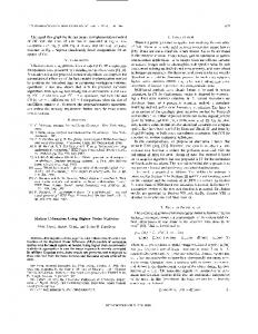
ROC curves on (a) ORL and (b) Yale Databases. Legend- Red (1): Our Method, Blue (2): KSVD, Green (3): Over-
complete DCT, Black (4): SSVD and (5): JPEG (Magenta). (c) Variance in RPP versus pre-quantization error for ORL. (d) Original image from ORL database. Sample reconstructions with δ = 3 × 10⁻⁴ of (d) by using (e) Our Method [RPP: 1.785, PSNR: 35.44], (f) KSVD [RPP: 2.112, PSNR: 35.37], (g) Over-complete DCT [RPP: 2.929, PSNR: 35.256], (h) SSVD [RPP: 2.69, PSNR: 34.578]. These plots are best viewed in color.
learned using the algorithm described in Section II-B. The T value for sparsity of the projection matrices was set to 10 during training. As shown in Figure III-D(c), we also computed the variance in the RPP values for every different pre-quantization error value, for each image in the ORL database. Note that the variance in RPP decreases with increase in specified error. This is because at very low errors, different images require different number of coefficients in order to meet the error. The same experiment was run on the Yale database with a value of T = 3 on patches of size 12 × 12. The training set consisted of a total of 64 images of one and the same person under different illumination conditions, whereas the testing set consisted of 65 images each of the remaining 38 people from the database (i.e. 2470 images in all), under different illumination conditions. The ROC curves for our method were superior to those of other methods over a significant range of δ, for the ORL as well as the Yale database, as seen in Figures 1(a) and 1(b). Sample reconstructions for an image from the ORL database are shown in Figures 1(d), 1(f), 1(g) and 1(h) for δ = 3 × 10⁻⁴ . For this image, our method produced a better PSNR to RPP ratio than others. Also Figure 2 shows reconstructed versions of another image from the ORL database using our method with different values of δ. For experiments on the March 20, 2009
DRAFT
SUBMITTED TO IEEE TRANSACTIONS ON IMAGE PROCESSING
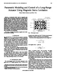
Fig. 2.
15
Original
Error 0.003
Error 0.001
Error 0.0005
Error 0.0003
Error 0.0001
Reconstructed versions of an image from the ORL database using 5 different error values. The original image is on
the extreme left and top corner.
ORL database, the number of bits used to code the fractional parts of the coefficients of the projection matrices [i.e. Q2 in Eqn. (12)] was set to 5. For the Yale database, we often obtained pre-quantization errors significantly less than the chosen δ, and hence using a value of Q2 less than 5 bits often did not raise the post-quantization error above δ. Keeping this in mind, we varied the value of Q2 dynamically, for each pre-quantization error value. The same variation was applied to the KSVD and over-complete DCT techniques as well. Furthermore, the dictionary size used by all the relevant methods being compared in the experiments here is shown in Table I. E. Effect of Different Parameters on the Performance of our Method: The different parameters in our method include: (1) the size of the patches for training and testing, (2) the number of pairs of orthonormal bases, i.e. K , and (3) the sparsity of each patch during training, i.e. T . In the following, we describe the effect of varying these parameters: 1) Patch Size: If the size of the patch is too large, it becomes more and more unlikely (due to the curse of dimensionality) that a fixed number of orthonormal matrices will serve as adequate bases for these patches in terms of a low-error sparse representation. Furthermore, if the patch size is March 20, 2009
DRAFT
SUBMITTED TO IEEE TRANSACTIONS ON IMAGE PROCESSING
16
Method
Dictionary Size (number of scalars)
Our Method
50 × 2 × 12 × 12 = 14400
KSVD
441 × 12 × 12 = 63504
Overcomplete DCT
441 × 12 × 12 = 63504
SSVD
-
JPEG
TABLE I
C OMPARISON OF DICTIONARY SIZE FOR VARIOUS METHODS FOR EXPERIMENTS ON THE ORL AND YALE DATABASES .
ORL: PSNR vs RPP; Diff. Values of T 40
35
35
PSNR
PSNR
ORL: PSNR vs. RPP, Diff. Patch Size 40
30 8X8 with T = 5 12X12 with T = 10 15X15 with T = 15 20X20 with T = 20
25
20 0
1
2
3
T=5 T = 10 T = 20 T = 50
25
4
RPP
(a) Fig. 3.
30
20 0
1
2
3
4
5
RPP
(b)
ROC curves for the ORL database using our technique with (a) different patch size and (b) different value of T for a
fixed patch size of 12 × 12. These plots are best viewed in color.
too large, any algorithm will lose out on the advantages of locality and simplicity. However, if the patch size is too small (say 2 × 2), there is very little a compression algorithm can do in terms of lowering the number of bits required to store these patches. We stress that the patch size as a free parameter is something common to all algorithms to which we are comparing our technique (including JPEG). Also, the choice of this parameter is mainly empirical. We tested the performance of our algorithm with K = 50 pairs of orthonormal bases on the ORL database, using patches of size 8 × 8, 12 × 12, 15 × 15 and 20 × 20, with appropriately chosen (different) values of T . As shown in Figure 3(a), the patch size of 12 × 12 using T = 10 yielded the best performance, though other patch sizes also performed quite well. 2) The number of orthonormal bases K : The choice of this number is not critical, and can be set to as high a value as desired without affecting the accuracy of the results, though it will increase the number of bits to store the basis index (see Eqn. 12). This parameter should not be confused with
March 20, 2009
DRAFT
SUBMITTED TO IEEE TRANSACTIONS ON IMAGE PROCESSING
17
the number of mixture components in standard mixture-model based density estimation, because in our method each patch gets projected only onto a single set of orthonormal bases, i.e. we do not compute a combination of projections onto all the K different orthonormal basis pairs. The only down-side of a higher value of K is the added computational cost during training. Again note that this parameter will be part of any learning-based algorithm for compression that uses a set of bases to express image patches. 3) The value of T during training: The value of T is fixed only during training, and is varied for each patch during the testing phase so as to meet the required error threshold. A very high value of T during training can cause the orthonormal basis pairs to overfit to the training data (variance),
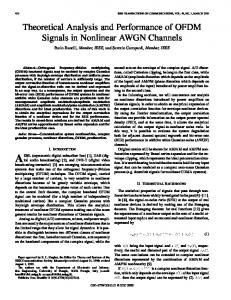
whereas a very low value could cause a large bias error. This is an instance of the well-known bias-variance tradeoff common in machine learning algorithms [35]. Our choice of T was empirical, though the value of T = 10 performed very well on nearly all the chosen datasets. The effect of different values of T on the compression performance for the ORL database is shown in Figure 3(b). We again emphasize that the issue with the choice of an ‘optimal’ T is not an artifact of our algorithm per se. For instance, this issue will also be encountered in pursuit algorithms to find the approximately optimal linear combination of unit vectors from a dictionary. In the latter case, however, there will also be the problem of poorer approximation errors as T increases, under certain conditions on the dictionary of overcomplete basis vectors [27]. F. Performance on Random Collections of Images We performed additional experiments to study the behavior of our algorithm when the training and test sets were very different from one another. To this end, we used the database of 155 natural images (in uncompressed format) from the Computer Vision Group at the University of Granada [36]. The database consists of images of faces, houses, natural scenery, inanimate objects and wildlife. We converted all the given images to grayscale. Our training set consisted of patches (of size 12 × 12) from 11 images. Patches from the remaining images were part of the test set. Though the images in the training and test sets were very different, our algorithm produced excellent results superior to JPEG upto an RPP value of 3.1 bits, as shown in Figure 4(a). Three training images and reconstructed versions of three different test images for error values of 0.0002, 0.0006 and 0.002 respectively, are shown in Figure III-F. To test the effect of minute noise on the performance of our algorithm, a similar experiment was run on the UCID database [37] with a training set of 10 images and the remaining 234 test images from the database. The test images were significantly different from the ones used for training. The images were scaled down March 20, 2009
DRAFT
SUBMITTED TO IEEE TRANSACTIONS ON IMAGE PROCESSING
18 UCID : RPP vs PSNR
40
CVG : RPP vs PSNR , T = 10 0
40 OurMethod
35
JPEG PSNR
PSNR
35
30
30
Our Method T =5 0
JPEG
25 25
20 0
0.5
1
1.5
2
2.5
3
20 0
3.5
(a) Fig. 4.
1
2
3
4
5
RPP
RPP
(b)
PSNR vs. RPP curve for our method and JPEG on (a) the CVG Granada database and (b) the UCID database.
by a factor of two (i.e. to 320 × 240 instead of 640 × 480) for faster training and subjected to zero mean Gaussian noise of variance 0.001 (on a scale from 0 to 1). Our algorithm was yet again competitive with JPEG as shown in Figure 4(b). IV. T HEORY: 3D ( OR
HIGHER -D) I MAGES
We now consider a set of images represented as third-order matrices (say RGB face images), each of size M1 × M2 × M3 . We divide each image into non-overlapping patches of size m1 × m2 × m3 , m1 ≪ M1 , m2 ≪ M2 , m3 ≪ M3 , and treat each patch as a separate tensor. Just as before, we start by exploiting
the similarity inherent in these patches, and represent them by means of sparse projections onto a triple of exemplar orthonormal bases. Again, we learn these exemplars a priori from a set of training image patches. We would like to point out that our extension to higher dimensions is non-trivial, especially when considering that a key property of the SVD in 2D (namely that SVD provides the optimal lowerrank reconstruction by simple nullification of the lowest singular values) does not extend into higherdimensional analogs such as HOSVD [18]. In the following, we now describe the mathematical structure of the exemplars. We would like to emphasize that though the derivations presented in this paper are for 3D matrices, a very similar treatment is applicable to learning n-tuples of exemplar orthonormal bases to represent patches from n-D matrices (where n ≥ 4). A. Exemplar Bases and Sparse Projections Let P ∈ Rm1 ×m2 ×m3 be an image patch. Using HOSVD, we can represent P as a combination of
orthonormal bases U ∈ Rm1 ×m1 , V ∈ Rm2 ×m2 and W ∈ Rm3 ×m3 in the form P = S ×1 U ×2 V ×3 W , March 20, 2009
DRAFT
SUBMITTED TO IEEE TRANSACTIONS ON IMAGE PROCESSING
19
(a)
(b)
(c)
(d)
(e)
(f)
(g)
(h)
(i)
(j)
(k)
(l)
Fig. 5. (a) to (c): Training images from the CVG Granada database. (d) to (l): Reconstructed versions of three test images for error values of 0.0002, 0.0006 and 0.002 respectively.
where S ∈ Rm1 ×m2 ×m3 is termed the core-tensor. The operators ×i refer to tensor-matrix multiplication over different axes. The core-tensor has special properties such as all-orthogonality and ordering. For further details of the core tensor and other aspects of multilinear algebra, the reader is referred to [18]. ¯ , V¯ and W ¯ , different Now, P can also be represented as a combination of any set of orthonormal bases U ¯ ×2 V¯ ×3 W ¯ where S is from those obtained from the HOSVD of P . In this case, we have P = S ×1 U
not guaranteed to be an all-orthogonal tensor, nor is it guaranteed to obey the ordering property. As the HOSVD does not necessarily provide the best low-rank approximation to a tensor [18], we choose to depart from this notion (instead of settling for a sub-optimal approximation), and instead answer the following question: What sparse tensor Q ∈ Rm1 ×m2 ×m3 will reconstruct P from a triple of
¯ , V¯ , W ¯ ) with the least error kP − Q×1 U ¯ ×2 V¯ ×3 W ¯ k2 ? Sparsity is again quantified orthonormal bases (U
by an upper bound T on the L0 norm of Q (denoted as kQk0 ). We now prove that the optimal Q with March 20, 2009
DRAFT
SUBMITTED TO IEEE TRANSACTIONS ON IMAGE PROCESSING
20
this sparsity constraint is obtained by nullifying the least (in absolute value) m1 m2 m3 − T elements of
¯ T ×2 V¯ T ×3 W ¯ T . Due to the ortho-normality of U ¯ , V¯ and the estimated projection tensor S = P ×1 U
¯ , this simple greedy algorithm turns out to be optimal (see Theorem 2). W
¯ ), the optimal sparse projection tensor Q with Theorem 2: Given a triple of orthonormal bases (U¯ , V¯ , W ¯ T ×2 V¯ T ×3 W ¯T kQk0 = T is obtained by setting to zero m1 m2 m3 −T elements of the tensor S = P ×1 U
having least absolute value. ¯ ×2 V¯ ×3 W ¯ . The error in reconstructing a patch P using some other matrix Q Proof: We have P = S ×1 U
¯ ×2 V¯ ×3 W ¯ k2 . For any tensor X , we have kXk2 = kX(n) k2 (i.e. the Frobenius norm is e = k(S −Q)×1 U
of the tensor and its nth unfolding are the same [18]). Also, by the matrix representation of HOSVD, we ¯ · S(n) · (V¯ ⊗ W ¯ )5 . Hence, it follows that e = kU ¯ · (S − Q)(1) · (V¯ ⊗ W ¯ )T k2 . This gives us have X(n) = U
¯ , V¯ and W ¯ , and hence V¯ ⊗ W ¯ are orthonormal matrices. e = kS − Qk2 . The last step follows because U P P 2 + Let I1 = {(i, j, k)|Qijk = 0} and I2 = {(i, j, k)|Qijk 6= 0}. Then e = (i,j,k)∈I1 Sijk (i,j,k)∈I2 (Sijk − Qijk )2 . This error will be minimized when Sijk = Qijk in all locations where Qijk 6= 0 and Qijk = 0 at
those indices where the corresponding values in S are as small as possible. Thus if we want kQk0 = T , then Q is the tensor obtained by nullifying m1 m2 m3 − T entries from S that have the least absolute value and leaving the remaining elements intact. We wish to re-emphasize that a key feature of our approach is the fact that the same technique used for 2D images scales to higher dimensions. Tensor decompositions such as HOSVD do not share this feature, because the optimal low-rank reconstruction property for SVD does not extend to HOSVD. Furthermore, though the upper and lower error bounds for core-tensor truncation in HOSVD derived in [24] are very interesting, they are applicable only when the entire set of images has a common basis (i.e. a common U , V and W matrix), which may not be sufficient to compactly account for the large variability in real-world
datasets.
B. Learning the Bases We now describe a method to learn K exemplar orthonormal bases {(Ua , Va , Wa )}, 1 ≤ a ≤ K , to
encode a training set of N image patches Pi ∈ Rm1 ×m2 ×m3 (1 ≤ i ≤ N ) with least possible error (in
the sense of the L2 norm of the difference between the original and reconstructed patches). Note that K ≪ N . In addition, we impose a sparsity constraint that every Sia (the tensor used to reconstruct Pi 5
Here A ⊗ B refers to the Kronecker product of matrices A ∈ RE1 ×E2 and B ∈ RF1 ×F2 , which is given as A ⊗ B =
(Ae1 e2 B)1≤e1 ≤E1 ,1≤e2 ≤E2 .
March 20, 2009
DRAFT
SUBMITTED TO IEEE TRANSACTIONS ON IMAGE PROCESSING
21
from (Ua , Va , Wa )) has at most T non-zero elements. The main objective function to be minimized is: E({Ua , Va , Wa , Sia , Mia }) =
N X K X i=1 a=1
Mia kPi − Sia ×1 Ua ×2 Va ×3 Wa k2
(13)
subject to the following constraints: (1) UaT Ua = VaT Va = WaT Wa = I, ∀a. (2) kSia k0 ≤ T, ∀(i, a). X (3) Mia = 1, ∀i, and Mia ∈ {0, 1}, ∀i, a.
(14)
a
Here Mia is a binary matrix of size N × K which indicates whether the ith patch belongs to the space defined by (Ua , Va , Wa ). Just as for the 2D case, we relax the binary membership constraint so that P now Mia ∈ (0, 1), ∀(i, a), subject to K a=1 Mia = 1, ∀i. Using Lagrange parameters {µi }, symmetric Lagrange matrices {Λ1a }, {Λ2a } and {Λ3a }, and a temperature parameter β , we obtain the following deterministic annealing objective function: E({Ua , Va , Wa , Sia , Mia }) =
N X K X i=1 a=1
Mia kPi − Sia ×1 Ua ×2 Va ×3 Wa k2 +
X X 1X Mia log Mia + µi ( Mia − 1) + β a ia i X X X T T trace[Λ1a (Ua Ua − I)] + trace[Λ2a (Va Va − I)] + trace[Λ3a (WaT Wa − I)]. a
a
(15)
a
We first initialize {Ua }, {Va } and {Wa } to random orthonormal tensors ∀a, and Mia =
1 K,
∀(i, a).
Secondly, using the fact that {Ua }, {Va } and {Wa } are orthonormal, the projection matrix Sia is computed by the rule: Sia = Pi ×1 UaT ×2 VaT ×3 WaT , ∀(i, a).
(16)
This is the minimum of the energy function kPi − Sia ×1 Ua ×2 Va ×3 Wa k2 . Then m1 m2 m3 − T elements in Sia with least absolute value are nullified. Thereafter, Ua , Va and Wa are updated as follows. Let us denote the sum of the terms in the previous energy function that are independent of Ua , as C . Then we can write the energy function as: E({Ua , Va , Wa , Sia , Mia }) =
=
X ia
X ia
Mia kPi − (Sia ×1 Ua ×2 Va ×3 Wa )k2 + X a
Mia kPi(1) − (Sia ×1 Ua ×2 Va ×3 Wa )(1) k2 + X a
March 20, 2009
trace[Λ1a (UaT Ua − I)] + C
trace[Λ1a (UaT Ua − I)] + C.
(17)
DRAFT
SUBMITTED TO IEEE TRANSACTIONS ON IMAGE PROCESSING
22
Note that here Pi(n) refers to the nth unfolding of the tensor Pi (refer to [18] for exact details). Also note that the above step uses the fact that for any tensor X , we have kXk2 = kX(n) k2 . Now, the objective function can be further expressed as follows: X E({Ua , Va , Wa , Sia , Mia }) = Mia kPi(1) − Ua · Sia(1) · (Va ⊗ Wa )T k2 + ia
X a
trace[Λ1a (UaT Ua − I)] + C. (18)
Further simplification gives:
X ia
E({Ua , Va , Wa , Sia , Mia }) = Mia trace[(Pi(1) − Ua · Sia(1) · (Va ⊗ Wa )T )T (Pi(1) − Ua · Sia(1) · (Va ⊗ Wa )T )] + X
=
X
a T Mia [trace[Pi(1) Pi(1) ]
ia
trace[Λ1a (UaT Ua − I)] + C
T − 2trace[Pi(1) Ua
T trace[Sia(1) Sia(1) )] +
X a
· Sia(1) · (Va ⊗ Wa )T ] +
trace[Λ1a (UaT Ua − I)] + C.
Taking the partial derivative of E w.r.t. Ua and setting it to zero, we have: X ∂E T = −2Mia Pi(1) (Va ⊗ Wa )Sia(1) + 2Ua Λ1a = 0. ∂Ua
(19)
(20)
i
After a series of manipulations to eliminate the Lagrange matrices, we arrive at the following update rule for Ua : ZU a =
X i
1
T Mia Pi(1) (Va ⊗ Wa )Sia(1) ; Ua = ZU a (ZUT a ZU a )− 2 = Γ1a ΥT1a .
(21)
Here Γ1a and Υ1a are orthonormal matrices obtained from the SVD of ZU a . The updates for Va and Wa are obtained similarly and are mentioned below: X 1 T ZV a = Mia Pi(2) (Wa ⊗ Ua )Sia(2) ; Va = ZV a (ZVT a ZV a )− 2 = Γ2a ΥT2a .
(22)
i
ZW a =
X i
1
T T −2 Mia Pi(3) (Ua ⊗ Va )Sia(3) = Γ3a ΥT3a . ; Wa = ZW a (ZW a ZW a )
(23)
Here again, Γ2a and Υ2a refer to the orthonormal matrices obtained from the SVD of ZV a , and Γ3a and Υ3a refer to the orthonormal matrices obtained from the SVD of ZW a . The membership values are obtained by the following update: 2
e−βkPi −Sia ×1 Ua ×2 Va ×3 Wa k . Mia = PK −βkPi −Sib ×1 Ub ×2 Vb ×3 Wb k2 b=1 e March 20, 2009
(24)
DRAFT
SUBMITTED TO IEEE TRANSACTIONS ON IMAGE PROCESSING
23
The core tensors {Sia } and the matrices {Ua , Va , Wa }, M are then updated sequentially for a fixed β value, until convergence. The value of β is then increased and the sequential updates are repeated. The entire process is repeated until an integrality condition is met.
C. Application to Compact Image Representation Quite similar to the 2D case, after the optimization during the training phase, each training patch Pi (1 ≤ i ≤ N ) gets represented as a projection onto one out of the K exemplar orthonormal bases, which
produces the least reconstruction error, i.e. the kth exemplar is chosen if kP − Sik ×1 Uk ×2 Vk ×3
Wk k2 ≤ kP − Sia ×1 Ua ×2 Va ×3 Wa k2 , ∀a ∈ {1, 2, ..., K}, 1 ≤ k ≤ K . For training patch Pi , we
denote the corresponding ‘optimal’ projection tensor as Si⋆ = Sik , and the corresponding exemplar as (Ui⋆ , Vi⋆ , Wi⋆ ) = (Uk , Vk , Wk ). Thus the entire set of patches can be closely approximated by (1) the
common set of basis-pairs {(Ua , Va , Wa )}, 1 ≤ a ≤ K (K ≪ N ), and (2) the optimal sparse projection tensors {Si⋆ } for each patch, with at most T non-zero elements each. The overall storage per image is
thus greatly reduced. Furthermore, these bases {(Ua , Va , Wa )} can now be used to encode patches from a new set of images that are similar to the ones existing in the training set, though just as in the 2D case, the sparsity of the patch will be adjusted dynamically in order to meet a given error threshold. Experimental results for this are provided in the next section. V. E XPERIMENTS : C OLOR I MAGES In this section, we describe the experiments we performed on color images represented in the RGB color scheme. Each image of size M1 × M2 × 3 was treated as a third-order matrix. Our compression algorithm was tested on the GaTech Face Database [38], which consists of RGB color images with 15 images each of 50 different people. The images in the database are already cropped to include just the face, but some of them contain small portions of a distinctly cluttered background. The average image size is 150 × 150 pixels, and all the images are in the JPEG format. For our experiments, we divided this database into a training set of one image each of 40 different people, and a test set of the remaining 14 images each of these 40 people, and all 15 images each of the remaining 10 people. Thus, the size of the test set was 710 images. The patch-size we chose for the training and test sets was 12 × 12 × 3 and we experimented with K = 100 different orthonormal bases learned during training. The value of T during training was set to 10. At the time of testing, for our method, each patch was projected onto that triple of orthonormal bases (Ui⋆ , Vi⋆ , Wi⋆ ) which gave the sparsest projection tensor Si⋆ such that the per-pixel reconstruction error March 20, 2009
kPi −Si ×1 Ui⋆ ×2 Vi⋆ ×3 Wi⋆ k2 m1 m2
was no greater than a chosen δ. Note that, in calculating the DRAFT
SUBMITTED TO IEEE TRANSACTIONS ON IMAGE PROCESSING
24
per-pixel reconstruction error, we did not divide by the number of channels, i.e. 3, because at each pixel, there are three values defined. We experimented with different reconstruction error values δ ranging from 8 × 10⁻⁵ to 8 × 10⁻³ . Following the reconstruction, the PSNR for the entire image was measured, and
averaged over the entire test test. The total number of bits per pixel, i.e. RPP, was also calculated for each image and averaged over the test set. The details of the training and testing methodology, and also the actual quantization and coding step are the same as presented previously in Section III-A and III-B. A. Comparisons with Other Methods The results obtained by our method were compared to those obtained by the following techniques: 1) KSVD, for which we used patches of size 12 × 12 × 3 reshaped to give vectors of size 432, and used these to train a dictionary of 1340 vectors using a value of T = 30. 2) Our algorithm for 2D images from Section II with an independent (separate) encoding of each of the three channels. As an independent coding of the R, G and B slices would fail to account for the inherent correlation between the channels (and hence give inferior compression performance), we used principal components analysis (PCA) to find the three principal components of the R, G, B values of each pixel from the training set. The R, G, B pixel values from the test images were then projected onto these principal components to give a transformed image in which the values in each of the different channels are decorrelated. A similar approach has been taken earlier in [39] for compression of color images of faces using vector quantization, where the PCA method is empirically shown to produce channels that are even more decorrelated than those from the Y-CbCr color model. The orthonormal bases were learned on each of the three (decorrelated) channels of the PCA image. This was followed by the quantization and coding step similar to that described in Section III-B. However in the color image case, the Huffman encoding step [34] for finding the optimal values of a1 , a2 and a3 in Eqn. (12) was performed using projection matrices from all three channels together. This was done to improve the coding efficiency. R 3) The JPEG standard (its MATLAB implementation), for which we calculated RPP from the number
of bytes of file storage on the disk. See Section V-B for more details. We would like to mention here that we did not compare our technique with [39]. The latter technique uses patches from color face images and encodes them using vector quantization. The patches from more complex regions of the face (such as the eyes, nose and mouth) are encoded using a separate vector quantization step for better reconstruction. The method in [39] requires prior demarcation of such regions, which in itself is a highly difficult task to automate, especially under varying illumination and pose. Our March 20, 2009
DRAFT
SUBMITTED TO IEEE TRANSACTIONS ON IMAGE PROCESSING
25
method does not require any such prior segmentation, as we manually tune the number of coefficients to meet the pre-specified reconstruction error. B. Results As can be seen from Figure 6(a), all three methods perform well, though the higher-order method produced the best results after a bit-rate of around 2 per pixel. For the GaTech database, we did not compare our algorithm directly with JPEG because the images in the database are already in the JPEG format. However, to facilitate comparison with JPEG, we used a subset of 54 images from the CMU-PIE database [40]. The CMU-PIE database contains images of several people against cluttered backgrounds with a large variation in pose, illumination, facial expression and occlusions created by spectacles. All the images are available in an uncompressed (.ppm) format, and their size is 631 × 467 pixels. We chose 54 images belonging to one and the same person, and used exactly one image for training, and all the remaining for testing. The results produced by our method using higher-order matrices, our method involving separate channels and also KSVD were seen to be competitive with those produced by JPEG. For a bit rate of greater than 1.5 per pixel, our methods produced performance that was superior to that of JPEG in terms of the PSNR for a given RPP, as seen in Figure V-B. The parameters for this experiment were K = 100 and T = 10 for training. Sample reconstructions of an image from the CMU-PIE database using our higher-order method for different error values are shown in Figure V-B. This is quite interesting, since there is considerable variation between the training image and the test images, as is clear from Figure V-B. We would like to emphasize that the experiments were carried out on uncropped images of the full size with the complete cluttered background. Also, the dictionary sizes for the experiments on each of these databases are summarized in Table II. For color-image patches of size m1 × m2 × 3 using K sets of bases, our method in 3D requires a dictionary of size 3Km1 m2 , whereas our method in 2D
requires a dictionary of size 2Km1 m2 per channel, which is 6Km1 m2 in total. C. Comparisons with JPEG on Noisy Datasets As mentioned before, we did not directly compare our results to the JPEG technique for the GaTech Face Database, because the images in the database are already in the JPEG format. Instead, we added zero-mean Gaussian noise of variance 8 × 10⁻⁴ (on a color scale of [0, 1]) to the images of the GaTech database and converted them to a raw format. Following this, we converted these raw images back to JPEG R (using MATLAB ) and measured the RPP and PSNR. These figures were pitted against those obtained
by our higher-order method, our method on separate channels, as well as KSVD, as shown in Figures March 20, 2009
DRAFT
SUBMITTED TO IEEE TRANSACTIONS ON IMAGE PROCESSING
35
PSNR
PSNR
40
30 Our Method: 3D Our Method: 2D KSVD
25 20 0
2
4
6
RPP
(a) Fig. 6.
PSNR vs RPP: Clean Training, Noisy Testing 32
32
30
30
28
28
26 24
Our Method: 3D Our Method: 2D KSVD JPEG
22 20 8
18 0
2
4
6
8
PSNR vs RPP: Noisy Training Noisy Testing
PSNR
PSNR vs RPP: Training and testing on clean images 45
26
26 24
Our Method (3D) Our Method (2D) KSVD JPEG
22 20 10
18 0
RPP
(b)
5
10
15
RPP
(c)
ROC curves for the GaTech database: (a) when training and testing were done on the clean original images, (b) when
training was done on clean images, but testing was done with additive zero mean Gaussian noise of variance 8 × 10⁻⁴ added to the test images, and (c) when training and testing were both done with zero mean Gaussian noise of variance 8 × 10⁻⁴ added to the respective images. The methods tested were our higher-order method, our method in 2D, KSVD and JPEG. Parameters for our methods: K = 100 and T = 10 during training. These plots are best viewed in color.
Training Image
Original Test Image
Error 0.003
Error 0.001
Error 0.0005
Error 0.0003
Error 0.0001
Fig. 7.
Sample reconstructions of an image from the CMU-PIE database with different error values using our higher order
method. The original image is on the top-left. These images are best viewed in color.
March 20, 2009
DRAFT
SUBMITTED TO IEEE TRANSACTIONS ON IMAGE PROCESSING
27
PSNR vs RPP: CMU−PIE 40
PSNR
35
30 Our Method (3D) Our Method (2D) KSVD JPEG
25
20 0
2
4
6
8
10
RPP
Fig. 8.
ROC curves for the CMU-PIE database using our method in 3D, our method in 2D, KSVD and JPEG. Parameters for
our methods: with K = 100 and T = 10 during training.These plots are best viewed in color.
Method
Dictionary Size (number of scalars)
Our Method (3D)
100 × 3 × 12 × 12 = 43200
Our Method (2D)
100 × 2 × 3 × 12 × 12 = 86400
KSVD
1340 × 12 × 12 × 3 = 578880
JPEG
TABLE II
C OMPARISON OF DICTIONARY SIZE FOR VARIOUS METHODS FOR EXPERIMENTS ON THE G AT ECH AND CMU-PIE DATABASES .
6(b) and 6(c). The performance of JPEG was distinctly inferior despite the fact that the noise added did not have a very high variance. The reason for this is that the algorithms used by JPEG use the fact that while representing most natural images, the lower frequencies strongly dominate. This assumption is invalid in case of sensor noise. Hence the DCT coefficients on noisy images will have prominently higher values, as a result of which JPEG produces higher bit rates for the same PSNR. For the purposes of comparison, we ran two experiments using our higher-order method, our separate channel method and KSVD as well. In the first experiment, noise was added only to the test set, though the orthonormal bases or the dictionary were learned on a clean training set (i.e. without noise being added to the training images). In the second experiment, noise was added to every image from the training set, and all methods were trained on these noisy images. The testing was performed on (noisy) images from the test set, and the ROC curves were plotted as usual. As can be seen from Figures 6(b) and 6(c), the PSNR values for JPEG begin to plateau off rather quickly. Note that in all these experiments, the PSNR is calculated from the squared difference between the reconstructed image and the noisy training image. This is because the March 20, 2009
DRAFT
SUBMITTED TO IEEE TRANSACTIONS ON IMAGE PROCESSING
28
‘original clean’ image would be usually unavailable in a practical application that required compression of noisy data. VI. C ONCLUSION We have presented a new technique for sparse representation of image patches, which is based on the notion of treating an image as a 2D entity. We go beyond the usual singular value decomposition of individual images or image-patches to learn a set of common, full-sized orthonormal bases for sparse representation, as opposed to low-rank representation. For the projection of a patch onto these bases, we have provided a very simple and provably optimal greedy algorithm, unlike the approximation algorithms that are part and parcel of projection pursuit techniques, and which may require restrictive assumptions on the nature or properties of the dictionary [27]. Based on the developed theory, we have demonstrated a successful application of our technique for the purpose of compression of two well-known face databases. Our compression method is able to handle the varying complexity of different patches by dynamically altering the number of coefficients (and hence the bit-rate for storage) in the projection matrix of the patch. Furthermore, this paper also presents a clean and elegant extension to higher order matrices, for which we have presented applications to color-image compression. Unlike decompositions like HOSVD which do not retain the optimal low-rank reconstruction property of SVD, our method scales cleanly into higher dimensions. The experimental results show that our technique compares very favorably to other existing approaches from recent literature, including the JPEG standard. We have also empirically examined the performance of our algorithm on noisy color image datasets. Directions for future work include: (1) investigation of alternative matrix representations tuned for specific applications (as opposed to using the default rows and columns of the image), (2) application of our technique for compression of gray-scale and color video (which can be represented as 3D and 4D matrices respectively), (3) application of our technique for denoising or classification, (4) a theoretical study of the method in the context of natural image statistics, and (5) a study on utilizing a perceptually driven quality metric [41] as opposed to a simple L2 norm. R EFERENCES [1] A. Rangarajan, “Learning matrix space image representations”, in Energy Minimization Methods in Computer Vision and Pattern Recognition (EMMCVPR). 2001, vol. 2134 of LNCS, pp. 153–168, Springer Verlag. [2] J. Ye, “Generalized low rank approximations of matrices”, Machine Learning, vol. 61, pp. 167–191, 2005. [3] J. Yang, D. Zhang, A. F. Frangi, and J. y. Yang, “Two-dimensional PCA: A new approach to appearance-based face representation and recognition”, IEEE Trans. Pattern Anal. Mach. Intell., vol. 26, no. 1, 2004. March 20, 2009
DRAFT
SUBMITTED TO IEEE TRANSACTIONS ON IMAGE PROCESSING
29
[4] X. He, D. Cai, and P. Niyogi, “Tensor subspace analysis”, in Neural Information Processing Systems, 2005, pp. 499–506. [5] H. C. Andrews and C. L. Patterson, “Singular value decomposition (SVD) image coding”, IEEE Transactions on Communications, pp. 425–432, 1976. [6] G. Golub and C. van Loan, Matrix Computations, The Johns Hopkins University Press, October 1996. [7] A. van der Schaaf and J. H. van Hateren, “Modelling the power spectra of natural images: statistics and information”, Vision Research, vol. 36, pp. 2759–2770, 1996. [8] J.-F. Yang and C.-L. Lu, “Combined techniques of singular value decomposition and vector quantization for image coding”, IEEE Transactions on Image Processing, vol. 4, no. 8, pp. 1141–1146, 1995. [9] C. Ding and J. Ye, “Two-dimensional singular value decomposition (2DSVD) for 2D maps and images”, in SIAM Int’l Conf. Data Mining, 2005, pp. 32–43. [10] G. Wallace, “The JPEG still picture compression standard”, IEEE Transactions on Consumer Electronics, vol. 38, no. 1, pp. 18–34, 1992. [11] B. Olshausen and D. Field, “Natural image statistics and efficient coding”, Network, vol. 7, pp. 333–339, 1996. [12] M. Lewicki, T. Sejnowski, and H. Hughes, “Learning overcomplete representations”, Neural Computation, vol. 12, pp. 337–365, 2000. [13] M. Aharon, M. Elad, and A. Bruckstein, “The K-SVD: An algorithm for designing of overcomplete dictionaries for sparse representation”, IEEE Transactions on Signal Processing, vol. 54, no. 11, pp. 4311–4322, November 2006. [14] P. Hoyer, “Non-negative matrix factorization with sparseness constraints”, Journal of Machine Learning Research, pp. 1457–1469, 2004. [15] D. Mallat and M. Avellaneda, “Adaptive greedy approximations”, Journal of Constructive Approximations, vol. 13, pp. 57–98, 1997. [16] K. Gurumoorthy, A. Rajwade, A. Banerjee, and A. Rangarajan,
“Beyond SVD - sparse projections onto exemplar
orthonormal bases for compact image representation”, in International Conference on Pattern Recognition (ICPR), 2008. [17] A. Shashua and A. Levin, “Linear image coding for regression and classification using the tensor-rank principle”, in CVPR(1), 2001, pp. 42–49. [18] L. de Lathauwer, B. de Moor, and J. Vandewalle, “A multilinear singular value decomposition”, SIAM J. Matrix Anal. Appl., vol. 21, no. 4, pp. 1253–1278, 2000. [19] J. H˚astad, “Tensor rank is NP-Complete”, in ICALP ’89: Proceedings of the 16th International Colloquium on Automata, Languages and Programming, 1989, pp. 451–460. [20] L. de Lathauwer, Signal Processing Based on Multilinear Algebra, PhD thesis, Katholieke Universiteit Leuven, Belgium, 1997. [21] M.A.O. Vasilescu and D. Terzopoulos, “Multilinear analysis of image ensembles: Tensorfaces”, in International Conference on Pattern Recognition (ICPR), 2002, pp. 511–514. [22] R. Costantini, L. Sbaiz, and S. Susstrunk, “Higher order SVD analysis for dynamic texture synthesis”, IEEE Transactions on Image Processing, vol. 17, no. 1, pp. 42–52, Jan. 2008. [23] H. Wang and N. Ahuja, “Rank-R approximation of tensors: Using image-as-matrix representation”, in IEEE Conference on Computer Vision and Pattern Recognition (CVPR), 2005, vol. 2, pp. 346–353. [24] C. Ding, H. Huang, and D. Luo, “Tensor reduction error analysis - applications to video compression and classification”, in IEEE Conference on Computer Vision and Pattern Recognition (CVPR), 2008.
March 20, 2009
DRAFT
SUBMITTED TO IEEE TRANSACTIONS ON IMAGE PROCESSING
30
[25] A. Ranade, S. Mahabalarao, and S. Kale, “A variation on SVD based image compression”, Image and Vision Computing, vol. 25, no. 6, pp. 771–777, 2007. [26] Y. Pati, R. Rezaiifar, and P. Krishnaprasad,
“Orthogonal matching pursuit: Recursive function approximation with
applications to wavelet decomposition”, in 27th Asilomar Conference on Signals, Systems and Computation, 1993, vol. 1, pp. 40–44. [27] J. Tropp, “Greed is good: algorithmic results for sparse approximation”, IEEE Transactions on Information Theory, vol. 50, no. 10, pp. 2231–2242, 2004. [28] C. Petersen and B. S¨oderberg, “A new method for mapping optimization problems onto neural networks”, International Journal of Neural Systems, vol. 1, pp. 3–22, 1989. [29] A. Yuille and J. Kosowsky, “Statistical physics algorithms that converge”, Neural Computation, vol. 6, no. 3, pp. 341–356, 1994. [30] R. Hathaway, “Another interpretation of the EM algorithm for mixture distributions”, Statistics and Probability Letters, vol. 4, pp. 53–56, 1986. [31] M. Tipping and C. Bishop, “Mixtures of probabilistic principal component analysers”, Neural Computation, vol. 11, no. 2, pp. 443–482, 1999. [32] “The ORL Database of Faces”, http://www.cl.cam.ac.uk/research/dtg/attarchive/facedatabase.html. [33] “The Yale Face Database”, http://cvc.yale.edu/projects/yalefaces/yalefaces.html. [34] D. Huffman, “A method for the construction of minimum-redundancy codes”, in Proceedings of the I.R.E., 1952, pp. 1098–1102. [35] S. Geman, E. Bienenstock, and R. Doursat, “Neural networks and the bias/variance dilemma”, Neural Computation, vol. 4, no. 1, pp. 1–58, 1992. [36] “The CVG Granada Database”, http://decsai.ugr.es/cvg/dbimagenes/index.php. [37] “The Uncompressed Colour Image Database”, http://vision.cs.aston.ac.uk/datasets/UCID/ucid.html. [38] “The Georgia Tech Face Database”, http://www.anefian.com/face reco.htm. [39] J. Huang and Y. Wang, “Compression of color facial images using feature correction two-stage vector quantization”, IEEE Transactions on Image Processing, vol. 8, pp. 102–109, 1999. [40] “The CMU Pose, Illumination and Expression (PIE) Database”, http://www.ri.cmu.edu/projects/project 418.html. [41] M. Eckert and A. Bradley, “Perceptual quality metrics applied to still image compression”, Signal Processing, vol. 70, no. 3, pp. 177–200, 1998.
March 20, 2009
DRAFT