Subsequence Search in Event-Interval Sequences Orestis Kostakis
Aristides Gionis
[email protected]
[email protected]
Aalto University Espoo, Finland
Aalto University Espoo, Finland
ABSTRACT We study the problem of subsequence search in databases of event-interval sequences, or e-sequences. In contrast to sequences of instantaneous events, e-sequences contain events that have a duration. In Information Retrieval applications, e-sequences are used for American Sign Language. We show that the subsequence-search problem is NP-hard and provide an exact (worst-case exponential) algorithm. We extend our algorithm to handle di↵erent cases of subsequence matching with errors. We then propose the Relation Index, a scheme for speeding up exact retrieval, which we benchmark against several indexing schemes.
1.
Figure 1: An event-interval sequence with 5 intervals.
INTRODUCTION
Figure 2: Event-interval sequences describe richer scenarios than symbolic sequences. Mapping event-interval sequences to symbolic sequences creates ambiguities.
Event-interval sequences, or e-sequences, are used in a plethora of real-world application domains, such as linguistics [2], sensor networks [6], and health informatics [7]. They are also used in information-retrieval applications for the American Sign Language (ASL) [5]. As a result, e-sequences have lately attracted considerable attention in both the database and knowledge-discovery communities. An example of an e-sequence is shown in Figure 1. In contrast to instantaneous event sequences, events in e-sequences have a duration. Hence, e-sequences convey richer information than instantaneous event sequences. It can be shown that information contained in e-sequences cannot be represented by instantaneous event sequences. Such an example is shown in Figure 2, where mapping e-sequences to symbolic sequences of instantaneous events creates ambiguity. Our experiments demonstrate that this type of representation error occurs in practice. In this paper we study the following problem: given a database D of e-sequences and a query e-sequence Q, find the e-sequences in D that contain Q. This problem applies, among others, to searching for specific phrases or grammatical constructions, among transcriptions of American Sign Language. Similarly, in Heath Informatics, a professional needs to search among medical records
for patients that exhibited symptoms in a specific combination; here we assume that event intervals are used to model conditions or medication states of patients. In this paper we make the following contributions: • We define the problem of subsequence matching, we prove that it is NP-hard, and we provide an exact algorithm. • We extend our algorithm to handle di↵erent cases of approximate subsequence matching. • We propose the Relation Index, a scheme for speeding up exact retrieval, which we benchmark against several indexing schemes.
2.
BACKGROUND
An event-interval sequence, or e-sequence, S = {S1 , . . . , S|S| } is a sequence of triples denoted Si = (Si .E, tstart , tend ). The coordinates of each triple denote the label, the starttime and end-time of each interval, respectively. For the example in Figure 1, the representation is S = {(A, 1, 10), (B, 5, 13), (C, 17, 30), (A, 20, 26), (D, 24, 30)}. We denote by |S| the length of S, which is the number of its intervals. Note that it is also possible to have overlapping intervals with the same label. Any pair of intervals in an e-sequence is characterized by a relation. The set of possible relations, based on Allen’s model [1], are shown in Figure 3. We only consider relations among intervals and ignore the absolute time durations. In American Sign Language, sentences are formed based on the combination of gestures not their duration: as with speaking, people may spend di↵er-
Permission to make digital or hard copies of all or part of this work for personal or classroom use is granted without fee provided that copies are not made or distributed for profit or commercial advantage and that copies bear this notice and the full citation on the first page. Copyrights for components of this work owned by others than the author(s) must be honored. Abstracting with credit is permitted. To copy otherwise, or republish, to post on servers or to redistribute to lists, requires prior specific permission and/or a fee. Request permissions from
[email protected]. SIGIR ’15, August 09 - 13, 2015, Santiago, Chile Copyright is held by the owner/author(s). Publication rights licensed to ACM. ACM 978-1-4503-3621-5/15/08 ...$15.00. http://dx.doi.org/10.1145/2766462.2767778
851
Algorithm 1 SubsequenceMatch
A
A
B
A meet B
A left-contain B
B
1: procedure SSM(Q, qPtr, S, sPtr, solSoFar) 2: if !S or !Q or sPtr > S.length() then 3: return false, solSoFar 4: for interval 2 S[sPtr,...] do 5: if Q[qPtr].label() = interval.label() then 6: compatible check relations(Q, qPtr, solSoFar, interval) 7: if !compatible then 8: continue 9: solSoFar.append(interval) 10: if qPtr = Q.length() 1 then 11: return true, solSoFar 12: else 13: (success,solSoFar) SSM(Q, qPtr, S, interval, solSoFar) 14: if success then 15: return true, solSoFar 16: else 17: solSoFar.pop() 18: return false, solSoFar
A
A A match B
B
A right-contain B
B
A
A B
A overlap B A
A contain B
B B
A follow B
Figure 3: The 7 temporal relations between event-intervals that are considered in this paper.
A B
S
C
A
T
A B C
Figure 4: S is a subsequence of T . the partial solution and is appended a new interval (line 9) or has an interval removed from the end (line 17); if Q is found in S, then upon termination solSoFar contains the corresponding intervals of S. Using this variable facilitates backtracking. Line 6 contains a check as to whether an interval in S, which has been found to have the same label as the next in Q, forms the same relations as those that are required by Q. |S| possible matchings between Q and S; There exist |Q| when all interval labels are the same. However, di↵erent labels and the backtracking due to interval relations eliminate a large number of candidates and reduce the running time.
ent time for gesturing the same phrase. Similarly, in robot sensor data, a high-level description of a situation is derived from the combination of relations of underlying events.
3.
SUBSEQUENCE MATCHING
Problem definition: An e-sequence S = {S1 , . . . , Sn } is a subsequence of T = {T1 , . . . , Tm } if S is contained in T . S is contained in T if and only if there exists a sequence T 0 of intervals, T 0 ✓ T , T 0 = {T10 , . . . , Tn0 }, such that Ti0 .E = Si .E, 1 i n and R(Si0 , Sj0 ) = R(Ti0 , Tj0 ), 1 i < j n, where R(·, ·) returns the relation between two intervals.
Problem variations: Algorithm 1 solves the problem of exact subsequence matching. However it can easily be modified to handle a number of variations, such as: • The sets of labels are considered equivalent. In other words, we do not require strict matching of labels, but instead we allow substitutions. This is easily implemented by replacing the equality condition of line 5 with the desired equivalence function. • A number of non-identical interval-relations are tolerated. In addition to solSoFar, we may use a second variable list that denotes how many relations with preceding intervals in solSoFar are violated when choosing solSoFar[i]. • A number of non-identical labels are tolerated. As above, we may use a variable list to maintain the errors. • Pathological matchings are avoided. As with the SakoeChiba Band [8] and the Itakura Parallelogram [4] for Dynamic Time Warping, we can force limits on the distance between consecutive intervals in S that get matched to Q. This is achieved by changing the limits of line 4.
Problem complexity: The subsequence matching problem (ssm) is NP-hard. This follows by a reduction from clique to ssm. The proof is omitted for space limitations. Theorem 1. Subsequence matching is NP-hard.
Note that in the special case that there is no overlap between intervals, the ssm problem can be solved in polynomial time, as it reduces to subsequence matching in strings. Another special case is to require that, for a query Q, the matched intervals in S are contiguous. This is also a polynomial variant, which can be solved in time O(|S||Q|2 ).
Algorithm: We present an exact algorithm, Algorithm 1, for determining if an e-sequence Q is a subsequence of S. The algorithm also returns the matching positions. It maintains a partial list that is used for backtracking. The algorithm scans the larger e-sequence S to find the first interval that shares the same label with the first interval in Q (lines 4,5). If such an interval is never found, the procedure will terminate. Suppose that an interval is found. As it is the first pair matched, no further checks are needed. Then, another interval with the same label as that of the second interval in Q is searched for in S. Searching for succeeding intervals happens recursively (line 13), for the remainders of the S and Q. A variable list solSoFar keeps
4.
INDEXING
When searching a very large dataset, sequential scan is prohibitive. An indexing scheme is required to improve the retrieval speed. We experiment with several approaches, each providing di↵erent trade-o↵s. We begin by describing the proposed indexing scheme, named Relation Index, while
852
Table 1: Dataset Summary.
Figure 5: A query using Relation Index decomposes an esequence into 2-interval structures. Linear variation enumerates only the top two, Quadratic enumerates all of them.
Dataset
# of e-seq.
max e-seq time
ASL Sensor Net Hepatitis
873 240 498
5957 284 7555
e-seq. length min max 4 47 15
41 149 592
# of classes 9 5 2
interval-labels, ordered in the same way as the intervals. For a query e-sequence Q to be a subsequence of an e-sequence S, it is a necessary, but not sufficient, requirement for the string representation of Q to be a subsequence of the string representation of S (easy proof omitted). All strings need to be examined, and the time complexity of each operation is O(|S|), hence the total time required for a single search is O(|D||S|). We may also transform e-sequences into strings as in Figure 2, but it creates sequences of double length. We refer to this scheme as Cpoint Index. Graph Indexing: We convert e-sequences to graphs, as described by Kostakis and Papapetrou [5], and then apply graph indexing techniques. We experimented with gIndex and FG-Index implementations provided by Han et al. [3].
the rest serve as baseline methods. All schemes guarantee a 100% recall rate: they return a superset of the valid result. Relation Index: this approach decomposes each e-sequence into a set of 2-interval e-sequences. Then it relies on an inverted index for performing look-ups. The keys in this inverted index are triples of the form (⌃i , ⌃j , relk ), with ⌃i , ⌃j 2 ⌃ and relk a type of relation. Each index key is associated with the list of e-sequence IDs that contain that specific combination. In the index-construction phase, for each e-sequence S 2 pairs of intervals and obtain their D, we enumerate all |S| 2 relation. For each formed triple (⌃i , ⌃j , relk ), the ID of that e-sequence is appended to the appropriate list in the index. In the retrieval phase, a set of interval pairs of the query esequence Q is enumerated, and the set of triples (⌃i , ⌃j , relk ) is produced. There are two approaches for choosing the set of interval pairs, as illustrated also in Figure 5: pairs are enumerated. 1. Quadratic: all |Q| 2 2. Linear : only |Q| 1 pairs are enumerated; those are extracted serially by examining only pairs of consecutive intervals, i.e. (Qi , Qi+1 ), 1 i |Q| 1. Given the set of produced triples, we first retrieve the cardinality of the index list of IDs for each key and we sort the keys in ascending order. The sorting helps speed-up the remainder of the process. Note that the set of values corresponding to the first key (the one with the fewer e-sequences containing that particular structure), is already a superset of the valid results for |Q|. Then, starting from the two smaller sets, we compute their intersection and then the intersection of the result with the third smallest set, etc. The process terminates when all intersections have been computed, or when the intersection contains at most one element.
5.
EXPERIMENTS
We evaluate the exact ssm algorithm and two of its variations on three real datasets, detailed in Table 1. The variations of ssm that we evaluated are the following: (i) a number of non-identical interval relations are tolerated, and (ii) a number of non-identical interval labels are toler] ated. The number of allowed errors takes values in [0, |Q| 2 for the case of relations, and in [0, |Q|] for the case of labels. In comparison to the exact ssm algorithm, these variations investigate more branches of the recursion tree, hence require longer run time. In addition, we expect a higher run time when we increase the number of allowed mismatches. Simply due to the fact that when the algorithm backtracks, this happens at a deeper stage. The expected size of the candidate set increases, too. We employ a synthetic dataset generator to create very large datasets for benchmarking the indexing methods. We create datasets of one million e-sequences and alphabet size, |⌃|, equal to 5, 50 and 500. Each e-sequence has length 100. The indexing methods are benchmarked in terms of retrieval time and size of returned candidate set. For all experiments, for each e-sequence in the dataset, we randomly select a number of intervals and query the dataset for the induced subsequence. The selected size ratios for |Q|/|S|, are 0.1, 0.2, 0.3, 0.5 and 0.99. Results on matching variations: Approximate matching with allowed relation errors was faster than the one with allowed label errors; by several orders of magnitude in some cases. Both were slower than the exact algorithm. As expected, the approximate e-sequence matching variations returned larger candidate sets than the exact version. In addition, the size increased with the allowed error rate. The same holds for the run times. Figure 6 depicts the results for the ASL dataset. For the Hepatitis and sensor network datasets the increase in run times was more significant. Indexing results: We witnessed that both gIndex and FGIndex are inefficient for the task at hand. Even for indexing a small dataset of 100 e-sequences with 100 intervals, both methods require over 1.5GB of memory. This is detrimental
Label Index: This approach is similar to the above, but it di↵ers in the type of keys. Instead of having an inverted index for sub-structures of two intervals, we simply create an inverted index for the interval labels. The two aforementioned approaches demonstrate a trade-o↵ between the size of the structures used as keys in the inverted index (the labels correspond to single intervals) and the index size. Bitmap Index: E-sequences are represented only by the count of each label of the intervals they contain. In order for a query e-sequence Q to be a subsequence of an e-sequence S, it is a necessary, but not sufficient, requirement for S to contain at least as many intervals of each label as those contained in Q. In order to provide fast lookup for each label count, we use hash tables. When searching in the Bitmap Index, each hash table needs to be examined. String Index: This is the baseline for indexing methods that map e-sequences to strings; each e-sequence in D is represented as a string. The tokens of the strings are the
853
−2
10
0.3 0.25 0.2 0.15 0.1 0.05
0
0.2
0.4
0.6
0.8
0 0
1
Query length
0.2
0.4
0.6
0.8
0.6 Relation (linear) Relation (quadratic) Bitmap String Label Cpoint
0.4 0.2
0.2
0.4
0.6
0.8
0
−2
10
−4
10
0.2
0.4
0.6
0.8
Query length
(a) Database size: 106
1
3
10
4
10
5
10
6
10
(b) Query length: 0.1
1
10 Relation (linear) Relation (quadratic) Bitmap String Label Cpoint
0.25 0.2 0.15 0.1 0.05 0 0
−6
10
−4
5
10
Database Size
6
Mean Query time (s)
−2
10
Candidates − ratio of DB
Mean Query Time (s)
10
0
4
10
Figure 8: Synthetic dataset |⌃| = 5. (a) Candidates size for variable query length, (b) run times for variable database size.
Relation (linear) Relation (quadratic) Bitmap String Label Cpoint
10
3
10
1
0.3 2
10
0
−2
10
(a) Database size: 106
ent values of allowed errors; ASL dataset. Same legend applies.
2
0
10
Query length
(b) Candidates
10
Relation (linear) Relation (quadratic) Bitmap String Label Cpoint
10
0 0
1
Figure 6: Benchmark of ssm algorithm and variations for di↵er-
Mean Query time (s)
0.8
Query length
(a) Query runtimes
10
10
−4
−3
10
Exact Relation Error 0.1 Relation Error 0.5 Relation Error 0.99 Label Error 0.1 Label Error 0.5 Label Error 0.99
Candidates − ratio of DB
Candidates − ratio of DB
Mean query time (s)
−1
10
2
1
0.4 0.35
Mean Query Time (s)
0
10
Database Size
−2
10
−3
0.4
0.6
0.8
1
(a) Database size: 106
(b) Query length: 0.1
Relation (linear) Relation (quadratic) Bitmap String Label Cpoint
−1
10
10 0.2
Query length
10
0
10
0
0.2
0.4
0.6
0.8
1
Query length
(b) Database size: 106
Figure 9: Synthetic dataset |⌃| = 50. (a) Candidates and (b)
Figure 7: Mean query run time for synthetic dataset, |⌃| = 500,
run times for variable query e-sequence length.
for variable (a) query e-sequence length and (b) database size.
6.
CONCLUSIONS
We studied the problem of subsequence search in databases of event-interval sequences, or e-sequences. We showed that the problem is NP-hard and provided an exact algorithm. We showed how to extend the exact algorithm to handle di↵erent cases of subsequence matching with errors. Finally, we proposed the Relation Index, a scheme that relies on decomposing e-sequences into pairs of intervals, for speeding up retrieval time. We benchmarked the proposed index against several baselines, including graph indexing schemes. We witness that Relation Index is superior in terms of run time compared to the other methods. While string indexing methods can be applied, they are inefficient for cases of small alphabet size. Between the linear and quadratic variants of Relation Index, the first is usually faster but the later is more efficient in pruning, when the alphabet size is small.
for scaling up to one million e-sequences. The reason is that an e-sequence of 100 intervals corresponds to a complete = 4950 edges. The number graph of 100 vertices, and 100·99 2 of edges is at least two orders of magnitude larger than those used by Han et al. [3]. Thus, we were unable to acquire any results for the datasets we experimented with. In general, the query times for String, Cpoint and Bitmap Index increase linearly with respect to the size of the database. As expected, this is due to the fact that they perform a linear scan and need to check all instances in D. For |⌃| = 500, all methods managed to find the single correct counterparts in all cases; precision 100%. Figure 7 shows the run times. Relation Index is two orders of magnitude faster than Bitmap Index and three orders faster than String Index. Due to the large alphabet size, each combination of interval labels appears few times, hence few lookups in the inverted index suffice to identify the unique candidate. For |⌃| = 5, for small query lengths the candidate sets are not singletons. In Figure 8 we notice that for query length ratio of 0.1, Bitmap and Label index compete in runtime with Relation Index but, including String and Cpoint Index, they are practically useless since they return the whole database. Only Relation Index is able to provide moderate pruning of the candidate set. The true candidate set is 27% of D, while Relation Index returns 60% of the DB. For |⌃| = 50, Relation Index remains at least an order of magnitude faster than the rest; Figure 9. Surprisingly, for small query lengths, it returns marginally more candidates than String Index. This is due to the fact that Relation Index retains no information on the location in the original e-sequence of the intervals involved in the relation. Hence, it may consider relations that do not correspond to the query’s location in the e-sequence. On the other hand, its query time decreases significantly for larger query lengths, because it performs fewer intersections.
References [1] J. F. Allen. Maintaining knowledge about temporal intervals. Communications of the ACM, 26(11):832–843, 1983. [2] B. Bergen and N. Chang. Embodied construction grammar in simulation-based language understanding. Construction grammars, pages 147–190, 2005. [3] W.-S. Han, J. Lee, M.-D. Pham, and J. X. Yu. iGraph: a framework for comparisons of disk-based graph indexing techniques. PVLDB, 3(1-2):449–459, 2010. [4] F. Itakura. Minimum prediction residual principle applied to speech recognition. IEEE Transactions on Acoustics, Speech & Signal Processing, 23(1):67–72, 1975. [5] O. Kostakis and P. Papapetrou. Finding the longest common sub-pattern in sequences of temporal intervals. Data Mining and Knowledge Discovery, pages 1–33, 2015. [6] F. Moerchen and D. Fradkin. Robust mining of time intervals with semi-interval partial order patterns. In SDM, 2010. [7] D. Patel, W. Hsu, and M. Lee. Mining relationships among interval-based events for classification. In SIGMOD, 2008. [8] H. Sakoe and S. Chiba. Dynamic programming algorithm optimization for spoken word recognition. IEEE Transactions on Signal Processing, 26(1):43–49, 1978.
854