Nov 14, 2006 - that switch pointers may not be used in conjunction with the ..... and G. Varghese, IP Lookup using Multi-way and Multi-column Search, IEEE.
Succinct Representation Of Static Packet Classifiers
∗
Wencheng Lu and Sartaj Sahni Department of Computer and Information Science and Engineering, University of Florida, Gainesville, FL 32611 {wlu, sahni}@cise.ufl.edu November 14, 2006
Abstract We develop algorithms for the compact representation of the 2-dimensional tries that are used for Internet packet classification. Our compact representations are experimentally compared with competing compact representations for multi-dimensional packet classifiers and found to simultaneously reduce the number of memory accesses required for a lookup as well as the memory required to store the classifier.
1
Introduction
An Internet router classifies incoming packets based on their header fields using a classifier, which is a table of rules. Each classifier rule is a pair (F, A), where F is a filter and A is an action. If an incoming packet matches a filter in the classifier, the associated action specifies what is to be done with this packet. Typical actions include packet forwarding and dropping. A d-dimensional filter F is a d-tuple (F [1], F [2], · · · , F [d]), where F [i] is a range that specifies destination addresses, source addresses, port numbers, protocol types, TCP flags, etc. A packet is said to match filter F , if its header field values fall in the ranges F [1], · · · , F [d]. Since it is possible for a packet to match more than one of the filters in a classifier, a tie breaker is used to determine a unique matching filter. Data structures for multi-dimensional (i.e., d > 1) packet classification are surveyed in [1]-[17]. Our focus in this paper is the succinct representation of the 2- and higher dimensional tries that are commonly used to represent multi-dimensional packet classifiers; the succinct representation is to support high-speed packet classification. For this work, we assume that the classifier is static. That is, the set of rules that comprise the classifier does not change (no inserts/deletes). This assumption is consistent with that made in most of the classifier literature where the objective is to develop a memory-efficient classifier representation that can be searched very fast. We begin, in Section 2, by reviewing the 1- and 2-dimensional binary trie representation of a classifier together with the research that has been done on the succinct representation of these structures. In Sections 3 through 5, we develop our our algorithms for the succinct representation of 2-dimensional tries. Experimental results are presented in Section 6. ∗ This
research was supported, in part, by the National Science Foundation under grant ITR-0326155
1
2
Background and Related Work
2.1
One-Dimensional Packet Classification
We assume that the filters in a 1-dimensional classifier are prefixes of destination addresses. Many of the data structures developed for the representation of a classifier are based on the binary trie structure [5]. A binary trie is a binary tree structure in which each node has a data field and two children fields. Branching is done based on the bits in the search key. A left child branch is followed at a node at level i (the root is at level 0) if the ith bit of the search key (the leftmost bit of the search key is bit 0) is 0; otherwise a right child branch is followed. Level i nodes store prefixes whose length is i in their data fields. The node in which a prefix is to be stored is determined by doing a search using that prefix as key. Let N be a node in a binary trie. Let Q(N ) be the bit string defined by the path from the root to N . Q(N ) is the prefix that corresponds to N . Q(N ) is stored in N.data in case Q(N ) is one of the prefixes to be stored in the trie. Several strategies–e.g., tree bitmap [3], shape shifting tries [15]–have been proposed to improve the lookup performance of binary tries. All of these strategies collapse several levels of each subtree of a binary trie into a single node, which we call a supernode, that can be searched with a number of memory accesses that is less than the number of levels collapsed into the supernode. For example, we can access the correct child pointer (as well as its associated prefix) in a multibit trie with a single memory access independent of the size of the multibit node. The resulting trie, which is composed of supernodes, is called a supernode trie. The data structure we propose in this paper also is a supernode trie structure. Our structure is most closely related to the shape shifting trie (SST) structure of Song et al. [15], which in turn draws heavily from the tree bitmap (TBM) scheme of Eatherton et al. [3] and the technique developed by Jacobson [6, 11] for the succinct representation of a binary tree. In TBM we start with the binary trie for our classifier and partition this binary trie into subtries that have at most S levels each. Each partition is then represented as a (TBM) supernode. S is the stride of a TBM supernode. While S = 8 is suggested in [3] for real-world IPv4 classifers, we use S = 2 here to illustrate the TBM structure. Fig. 1 (a) shows a partitoning of a binary trie into 4 subtries W–Z that have 2 levels each. Although a full binary trie with S = 2 levels has 3 nodes, X has only 2 nodes and Y and Z have only one node each. Each partition is is represented by a supernode (Fig. 1 (b)) that has the following components: 1. A (2S − 1)-bit bit map IBM (internal bitmap) that indicates whether each of the up to 2S − 1 nodes in the partition contains a prefix. The IBM is constructed by superimposing the partition nodes on a full binary trie that has S levels and traversing the nodes of this full binary trie in level order. For node W, the IBM is 110 indicating that the root and its left child have a prefix and the root’s right child is either absent or has no prefix. The IBM for X is 010, which indicates that the left child of the root of X has a prefix and that the right child of the root is either absent or has no prefix (note that the root itself is always present and so a 0 in the leading position of an IBM indicates that the root has no prefix). The IBM’s for Y and Z are both 100. 2
W
a
W
0 0
d
X
1
c
b 0
IBM: 110 EBM: 1011
1
e
f
Y
Z
child pointer X
pointer Y
H1 H2 Z
IBM: 010 IBM: 100 IBM: 100 EBM: 0000 EBM: 0000 EBM: 0000
0
g
next hop
H3
(a) TBM partitioning
H4
H5
(b) TBM node representation
Figure 1: TBM example 2. A 2S -bit EBM (external bit map) that corresponds to the 2S child pointers that the leaves of a full S-level binary trie has. As was the case for the IBM, we superimpose the nodes of the partition on a full binary trie that has S levels. Then we see which of the partition nodes has child pointers emanating from the leaves of the full binary trie. The EBM for W is 1011, which indicates that only the right child of the leftmost leaf of the full binary trie is null. The EBMs for X, Y and Z are 0000 indicating that the nodes of X, Y and Z have no children that are not included in X, Y, and Z, respectively. Each child pointer from a node in one partition to a node in another partition becomes a pointer from a supernode to another aupercode. To reduce the space required for these inter-supernode pointers, the children supernodes of a supernode are stored sequentially from left to right so that using the location of the first child and the size of a supernode, we can compute the location of any child supernode. 3. A child pointer that points to the location where the first child supernode is stored. 4. A pointer to a list N H of next-hop data for the prefixes in the partition. N H may have up to 2S − 1 entries. This list is created by traversing the partition nodes in level order. The N H list for W is nh(P 1) and nh(P 2), where nh(P 1) is the next hop for prefix P 1. The N H list for X is nh(P 3). While the N H pointer is part of the supernode, the N H list is not. The N H list is conveniently represented as an array. The N H list (array) of a supernode is stored separate from the supernode itself and is accessed only when the longest matching prefix has been determined and we now wish to determine the next hop associated with this prefix. If we need b bits for a pointer, then a total of 2S+1 + 2b − 1 bits (plus space for an N H list) are needed for each TBM supernode. Using the IBM, we can determine the longest matching prefix in a supernode; the EBM is used to determine whether we should move next to the first, second, etc. child of the current supernode. If a single memory access is sufficient to retrieve an entire supernode, we can move from one supernode to its child with a single access. The total number of memory accesses to search a supernode trie becomes the number of levels in the supernode trie plus 1 (to access the next hop for the longest matching prefix). The SST supernode structure proposed by Song et al. [15] is obtained by partitioning a binary trie into subtries that have at most K nodes each. K is the stride of an SST supernode. To correctly search an SST, each SST
3
supernode requires a shape bit map (SBM) in addition to an IBM and EBM. The SBM used by Song et al. [15] is the succinct representation of a binary tree developed by Jacobson [6]. Jacobson’s SBM is obtained by replacing every null link in the binary tree being coded by the SBM with an external node. Next, place a 0 in every external node and a 1 in every other node. Finally, traverse this extended binary tree in level order, listing the bits in the nodes as they are visited by the traversal. X SBM: 1010 IBM: 110 EBM: 1010
a X
0 0
d
1
c
b 0
e
1
Y
Y
H1 H2
Z
SBM: 1100 SBM: null IBM: 011 IBM: 1 EBM: 0000 EBM: 00
f
0
g Z
H4 H5
(a) SST partitioning
H3
(b) SST node representation
Figure 2: SST for binary trie of Fig. 1 (a) Suppose we partition our example binary trie of Fig. 1 (a) into binary tries that have at most K = 3 nodes each. Fig. 2 (a) shows a possible partitioning into the 3 partitions X-Z. X includes nodes a, b and d of Fig. 1 (a); Y includes nodes c, e and f; and Z includes node g. The SST representation has 3 (SST) supernodes. The SBMs for the supernodes for X-Z, respectively, are 1101000, 1110000, and 100. Note that a binary tree with K internal nodes has exactly K + 1 external nodes. So, when we partition into binary tries that have at most K internal nodes, the SBM is at most 2K + 1 bits long. Since the first bit in an SBM is 1 and the last 2 bits are 0, we don’t need to store these bits explicitly. Hence, an SBM requires only 2K − 2 bits of storage. Fig. 2 (b) shows the node representation for each partition of Fig. 2 (a). The shown SBMs exclude the first and last two bits. The IBM of an SST supernode is obtained by traversing the partition in level order; when a node is visited, we ouput a 1 to the IBM if the node has a prefix and a 0 otherwise. The IBMs for nodes X-Z are, respectively, 110, 011, and 1. Note than the IBM of an SST supernode is at most K bits in length. To obtain the EBM of a supernode, we start with the extended binary tree for the partition and place a 1 in each external node that corresponds to a node in the original binary trie and a 0 in every other external node. Next, we visit the external nodes in level order and output their bit to the EBM. The EBMs for our 3 supernodes are, respectively, 1010, 0000, and 00. Since the number of external nodes for each partition is at most K + 1, the size of an EBM is at most K + 1 bits. As in the case of the TBM structure, child supernodes of an SST supernode are stored sequentially and a pointer to the first child supernode maintained. The N H list for the supernode is stored in separate memory and a pointer to this list maintained within the supernode. Although the size of an SBM, IBM and EBM varies with the partition size, an SST supernode is of a fixed size and allocates 2K bits to the SBM, K bits to the IBM and K + 1 bits to the EBM. Unused bits are filled with 0s. Hence, the size of an SST supernode is 4K + 2b − 1 bits. 4
Song et al. [15] develop an O(m) time algorithm, called post-order pruning, to construct a minimum-node SST, for any given K, from an m-node binary trie. They develop also a breadth-first pruning algorithm to construct, for any given K, a minimum height SST. The complexity of this algorithm is O(m2 ). Lu and Sahni [10] developed an improved algorithm, which reduces the complexity of minimum height SST construction to O(m). For dense binary tries, TBMs are more space efficient than SSTs. However, for sparse binary tries, SSTs are more space efficient. Song et al. [15] propose a hybrid SST (HSST) in which dense subtries of the overall binary trie are partitioned into TBM supernodes and sparse subtries into SST supernodes. Fig. 3 shows an HSST for the binary trie of Fig. 1 (b). For this HSST, K = S = 2. The HSST has two SST nodes X and Z, and one TBM node Y. X SBM: 10 IBM: 11 EBM: 110
a
X
1
0 0
d
H1 H2
b
c 0
e
Y
Z
IBM: 011 SBM: 10 EBM: 0000 IBM: 01 EBM: 000
1
f
0 Z
Y
g
H4 H5
(a) HSST partitioning
H3
(b) HSST node representation
Figure 3: HSST for binary trie of Fig. 1(a) Although Song et al. [15] do not develop an algorithm to construct a space-optimal HSST, they propose a heuristic that is a modification of their breadth-first pruning algorithm for SSTs. This heuristic guarantees that the height of the constructed HSST is no more than that of the height-optimal SST. Lu and Sahni [10] developed dynamic programming formulations for the construction of space-optimal HSSTs.
2.2
Two-Dimensional Packet Classification
We assume that the filters are of the form (D, E), where D is a destination address prefix and E is a source address prefix. A 2-dimensional classifier may be represented as a 2-dimensional binary trie (2DBT), which is a one-dimensional binary trie (called the top-level trie) in which the data field of each node is a pointer to a (possibly empty) binary trie (called the lower-level trie). So, a 2DBT has 1 top-level trie and potentially many lower-level tries. Consider the 5-rule two-dimensional classifier of Figure 4(a). For each rule, the filter is defined by the Dest (destination) and Source prefixes. So, for example, F 2 = (0∗, 1∗) matches all packets whose destination address begins with 0 and whose source address begins with 1. When a packet is matched by two or more filters, the matching rule with least cost is used. The classifier of Figure 4(a) may be represented as a 2DBT in which the top-level trie is constructed using the destination prefixes. In the context of our destination-source filters, this top-level trie is called the destination trie (or simply, dest trie). Let N be a node in the destination trie. If no 5
a
1
0 b 0 1
d
c 0
1
e
f
0 F1
0
F2
g 1
0
Filter F1 F2 F3 F4 F5
Dest Prefix * 0* 000* 10* 11*
Source Prefix 0* 1* 0* 0* 1*
F4
F5
0
Cost 1 2 3 4 5
F3
dest tree node source tree node
(b) Corresponding two-dimensional binary trie
(a) 5 prefixes
Figure 4: Prefixes and corresponding two-dimensional binary trie dest prefix equals Q(N ), then N.data points to an empty lower-level trie. If there is a dest prefix D that equals Q(N ), then N.data points to a binary trie for all source prefixes E such that (D, E) is a filter. In the context of destination-source filters, the lower-level tries are called source trees. Every node N of the dest trie of a 2DBT has a (possibly empty) source trie hanging from it. Let a and b be two nodes in the dest trie. Let b be an ancestor of a. We say that the source trie that hangs from b is an ancestor trie of the one that hangs from a. Figure 4(b) gives the 2DBT for the filters of Figure 4(a). Srinivasan and Varghese [13] proposed using two-dimensional one-bit tries, a close relative of 2DBTs, for destination-source prefix filters. The proposed two-dimensional trie structure takes O(nW ) memory, where n is the number of filters in the classifier and W is the length of the longest prefix. Using this structure, a packet may be classified with O(W 2 ) memory accesses. The basic two-dimensional one-bit trie may be improved upon by using pre-computation and switch pointers [13]. The improved version classifies a packet making only O(W ) memory accesses. Srinivasan and Varghese [13] also propose extensions to higher-dimensional one-bit tries that may be used with d-dimensional, d > 2, filters. Baboescu et al. [2] suggest the use of two-dimensional one-bit tries with buckets for d-dimensional, d > 2, classifiers. Basically, the destination and source fields of the filters are used to construct a two-dimensional one-bit trie. Filters that have the same destination and source fields are considered to be equivalent. Equivalent filters are stored in a bucket that may be searched serially. Baboescu et al. [2] report that this scheme is expected to work well in practice because the bucket size tends to be small. They note also that switch pointers may not be used in conjunction with the bucketing scheme. Lu and Sahni [8], develop fast polynomial-time algorithms to construct space-optimal constrained 2DMTs (twodimensional multibit tries). The constructed 2DMTs may be searched with at most k memory accesses, where k is a design parameter. The space-optimal constrained 2DMTs of Lu and Sahni [8] may be used for d-dimensional filters, d > 2, using the bucketing strategy proposed in [2]. For the case d = 2, switch pointers may be employed 6
to get multibit tries that require less memory than required by space-optimal constrained 2DMTs and that permit packet classification with at most k memory accesses. Lu and Sahni [8] develop also a fast heuristic to construct good multibit tries with switch pointers. Experiments reported in [8] indicate that, given the same memory budget, space-optimal constrained 2DMT structures perform packet classification using 1/4 to 1/3 as many memory accesses as required by the two-dimensional one-bit tries of [13, 2].
3
Space-Optimal 2DHSSTs
Let T be a 2DBT. We assume that the source tries of T have been modified so that the last prefix encountered on each search path is the least-cost prefix for that search path. This modification is accomplished by examining each source-trie node N that contains a prefix and replacing the contained prefix with the least-cost prefix on the path from the root to N . A 2DHSST may be constructed from T by partitioning the top-level binary trie (i.e., the dest trie) of T and each lower-lever binary trie into a mix of TBM and SST supernodes. Supernodes that cover the top-level binary trie use their N H (next hop) lists to store the root supernodes for the lower-level HSSTs that represent lower-level tries of T . Figure 5 shows a possible 2DHSST for the 2DBT of Figure 4(b). The supernode strides used are K = S = 2. A 2DHSST may be searched for the least-cost filter that matches any given pair of destination and source addresses (da, sa) by following the search path for da in the destination HSST of the 2DHSST. All source tries encountered on this path are searched for sa. The least-cost filter on these source-trie search paths that matches sa is returned. Suppose we are to find the least-cost filter that matches (000,111). The search path for 000 takes us first to the root (ab) of the 2DHSST of Figure 5 and then to the left child (dg). In the 2DHSST root, we go through nodes a and b of the dest binary trie and in the supernode dg, we go through nodes d and g of T . Three of the encountered nodes (a, b, and g) have a hanging source trie. The corresponding source HSSTs are searched for 111 and F2 is returned as the least-cost matching filter.
a 0 b 0 1
d
1 c 0 e
0
1
F1
f
0
F2
g 0 F4
1 F5
0 F3
Figure 5: Two-dimensional supernode trie for Figure 4(a)
7
To determine the number of memory accesses required by a search of a 2DHSST, we assume sufficient memory bandwidth that an entire supernode (this includes the IBM, EBM, child and N H pointers) may be accessed with a single memory reference. To access a component of the N H array, an additional memory access is required. For each supernode on the search path for da, we make one memory access to get the supernode’s fields (e.g., IBM, EBM, child and N H pointers). In addition, for each supernode on this path, we need to examine some number of hanging source HSSTs. For each source HSST examined, we first access a component of the dest-trie supernode’s N H array to get the root of the hanging source HSST. Then we search this hanging source HSST by accessing the remaining nodes on the search path (as determined by the source address) for this HSST. Finally, the N H component corresponding to the last node on this search path is accessed. So, in the case of our above example, we make 2 memory accesses to fetch the 2 supernodes on the dest HSST path. In addition, 3 source HSSTs are searched. Each requires us to access its root supernode plus an N H component. in each source HSST. The total number of memory accesses is 2 + 2 ∗ 3 = 8. Let M N M A(X) be the maximum number of memory accesses (MNMA) required to search a source HSST X. For a source HSST, the MNMA includes the access to N H component of the last node on the search path. So, M N M A(X) is one more than the number of levels in X. Let U be a 2DHSST for T with strides S and K. Let P be any root to leaf path in the top level HSST of U . Let the sum of the MNMAs for the lower-level HSSTs on the path P be H(P ). Let nodes(P ) be the number of supernodes on the path P . Define 2DHSST (h) to be the subset of the possible 2DHSSTs for T for which max{H(P ) + nodes(P )} ≤ h P
(1)
Note that every U, U ∈ 2DHSST (h), can be searched with at most h memory accesses per lookup. Note also that some 2DHSSTs that have a path P for which H(P ) + nodes(P ) = h can be searched with fewer memory accesses than h as there may be no (da, sa) that causes a search to take the longest path through every source HSST on paths P for which H(P ) + nodes(P ) = h. We consider the construction of a space-optimal 2DHSST V such that V ∈ 2DHSST (H). We refer to such a V as a space-optimal 2DHSST (h). Let N be a node in T ’s top-level trie, and let 2DBT (N ) be the 2-dimensional binary trie rooted at N . Let opt1(N, h) be the size (i.e., number of supernodes) of the space-optimal 2DHSST (h) for 2DBT (N ). opt1(root(T ), H) gives the size of a space-optimal 2DHSST (H) for T . Let g(N, q, h) be the size (excluding the root) of a space-optimal 2DHSST (h) for 2DBT (N ) under the constraint that the root of the 2DHSST is a TBM supernode whose stride is q. So, g(N, S, h) + 1 gives the size of a space-optimal 2DHSST (h) for 2DBT (N ) under the constraint that the root of the 2DHSST is a TBM supernode whose stride is S. We see that, for q > 0, g(N, q, h) =
min
{g(LC(N ), q − 1, h − i) + g(RC(N ), q − 1, h − i) + s(N, i)}
m(N )≤i≤h
(2)
where m(N ) is the minimum possible value of MNMA for the source trie (if any) that hangs from the node N (in case there is no source trie hanging from N , m(N ) = 0), g(N, 0, h) = opt1(N, h − 1), g(null, t, h) = 0, and LC(N ) 8
and RC(N ) respectively, are the left and right children (in T ) of N . s(N, i) is the size of the space-optimal HSST for the source trie that hangs off from N under the constraint that the HSST has an MNMA of at most i. s(N, i) is 0 if N has no hanging source trie. Let opt1(N, h, k) be the size of a space-optimal 2DHSST (h) for 2DBT (N ) under the constraint that the root of the 2DHSST is an SST supernode whose utilization is k. It is easy to see opt1(N, h) = min{g(N, S, h) + 1, min {opt1(N, h, k)}} 0 0 and h > 0. If N has no child, opt1(N, h, k) = 1 + s(N, h − 1)
(4)
When N has only one child a, opt1(N, h, k) =
min
{f (a, h − i, k − 1) + s(N, i)}
m(N )≤i 0 and 1 + opt1(N, h − 1, 0) when k = 0. When N has two children a and b, opt1(N, h, k) =
min
{ min {f (a, h − i, j) + f (b, h − i, k − j − 1) − 1} + s(N, i)}
m(N )≤i