Hindawi Mathematical Problems in Engineering Volume 2017, Article ID 3513980, 7 pages https://doi.org/10.1155/2017/3513980
Research Article Sunspots Time-Series Prediction Based on Complementary Ensemble Empirical Mode Decomposition and Wavelet Neural Network Guohui Li and Siliang Wang School of Electronic Engineering, Xi’an University of Posts and Telecommunications, Xi’an, Shaanxi 710121, China Correspondence should be addressed to Guohui Li;
[email protected] Received 25 January 2017; Accepted 2 March 2017; Published 16 March 2017 Academic Editor: Tomasz Kapitaniak Copyright © 2017 Guohui Li and Siliang Wang. This is an open access article distributed under the Creative Commons Attribution License, which permits unrestricted use, distribution, and reproduction in any medium, provided the original work is properly cited. The sunspot numbers are the major target which describes the solar activity level. Long-term prediction of sunspot activity is of great importance for aerospace, communication, disaster prevention, and so on. To improve the prediction accuracy of sunspot time series, the prediction model based on complementary ensemble empirical mode decomposition (CEEMD) and wavelet neural network (WNN) is proposed. First, the sunspot time series are decomposed by CEEMD to obtain a set of intrinsic modal functions (IMFs). Then, the IMFs and residuals are reconstructed to obtain the training samples and the prediction samples, and these samples are trained and predicted by WNN. Finally, the reconstructed IMFs and residuals are the final prediction results. Five kinds of prediction models are compared, which are BP neural network prediction model, WNN prediction model, empirical mode decomposition and WNN hybrid prediction model, ensemble empirical mode decomposition and WNN hybrid prediction model, and the proposed method in this paper. The same sunspot time series are predicted with five kinds of prediction models. The experimental results show that the proposed model has better prediction accuracy and smaller error.
1. Introduction The sunspot numbers are the major targets which describes the solar activity level. The solar activity influences the human health and living environment on earth. Long-term prediction of sunspot activity can provide important reference information for aerospace, communication, disaster prevention, and so on [1]. Therefore, the research of sunspot number time-series prediction method has been an important and hot topic in this field [2]. The data of annual and monthly sunspot activity is considered as typical nonlinear, non-Gaussian, and nonstationary time series, which has obvious characteristics of chaotic sequences [3, 4]. The accurate prediction of sunspot numbers has great research significance [5, 6]. It is difficult to predict using the traditional method and the accuracy is not high. Currently, BP neural network, wavelet neural network, and empirical mode decomposition (EMD) [7] are widely used in nonlinear, nonstationary time-series prediction [8]. BP neural network has some advantages such as simple
structure, strong learning ability, and nonlinear mapping ability. But the predict model of BP neural network is easy to fall into the local minimum problem, and the convergence rate is slow [9]. Wavelet neural network is combined with the characteristics of artificial neural network and wavelet analysis. It has the advantages of self-learning ability and localization of wavelet transform, so it can effectively solve the local minimum problem [10]. In [11], tight wavelet neural network is used to predict sunspot number. Wavelet neural network is used to predict the charge load in [12]. It is shown that wavelet neural network obviously improves the prediction accuracy compared with BP neural network model. In [13], EMD is used to extract a signal which is more stable, and then the wavelet analysis method is used to get key features of sunspot data time series. However, the mode mixing effect will happen in the process of decomposing signal by the EMD, which leads to unsatisfactory decomposition. Wu and Huang [14] proposes ensemble empirical mode decomposition (EEMD) which is a noise-assisted data analysis method, and the mode mixing can be avoided during the empirical
2
Mathematical Problems in Engineering
𝜔ij
Φ(x)
.. .
(3) Decompose 𝑟1 (𝑡)+𝜀1 𝐸1 (𝜔𝑖 (𝑡)), 𝑖 = 1, 2, . . . , 𝑛. The first intrinsic modal function is used as the IMF2 of the CEEMD:
Φ(x) 𝜔jk
IMF2 (𝑡) = .. .
.. .
.. .
X(i)
hj
m Input layer
n Output layer
𝑟𝑘 (𝑡) = 𝑟𝑘−1 (𝑡) − IMF𝑘 (𝑡) .
Yk
IMF(𝑘+1) (𝑡) =
Figure 1: The structure of wavelet neural network.
1 𝑛 ∑𝐸 (𝑟 (𝑡) + 𝜀𝑘 𝐸𝑘 (𝜔𝑘 (𝑡))) . 𝑛 𝑖=1 1 𝑘
(5)
(6) Repeat steps (4) and (5), until the residual can no longer be decomposed, and then the final residuals 𝑅(𝑡) is
mode decomposition [15]. In [16], the mix model with EEMD and wavelet neural network is proposed. Although the reconstruction error is reduced, the cost of computing is increased [17]. Yeh et al. [18] propose complementary ensemble empirical mode decomposition. The method adds different Gaussian white noise to the remaining components of each intrinsic mode functions to reduce the mode mixing and decrease false component. Therefore, the prediction model based on complementary ensemble empirical mode decomposition and wavelet neural network is proposed, which is combined with the advantages of CEEMD and wavelet neural network and adopts the idea of a combined model.
2. Basic Principle 2.1. Complementary Ensemble Empirical Mode Decomposition. CEEMD is a noise-assisted analysis method [19]. Two opposite white noise signals are added to the time series signal, and 𝑗th mode is obtained by the EMD. 𝐸𝑗 (⋅) represents the 𝑗th intrinsic modal function of the EMD. 𝜔𝑖 (𝑛) represents zero mean Gaussian white noise with unit variance, that is, 𝑁(0, 1). 𝜀𝑘 represents the signal-to-noise ratio which is selected for each stage. 𝑥(𝑡) is set as target signal, and then the signal added to white noise is 𝑥(𝑡) + 𝜀0 𝜔𝑖 (𝑛). The concrete steps of the CEEMD algorithm [20] are as follows: (1) Decompose 𝑥(𝑡) + 𝜀0 𝜔𝑖 (𝑛) by the EMD for 𝑁 times, then IMF1 is obtained: (1)
(2) Calculate the first-order residual 𝑟1 : 𝑟1 (𝑡) = 𝑥 (𝑡) − IMF1 (𝑡) .
(4)
(5) Decompose 𝑟𝑘 (𝑡) + 𝜀𝑘 𝐸𝑘 (𝜔𝑘 (𝑡)). The first intrinsic modal function is used as the IMF(𝑘+1) of the CEEMD:
s Hidden layer
1 𝑛 ∑IMF𝑖1 (𝑡) . 𝑁 𝑖=1
(3)
(4) In the same way, the 𝑘th residual 𝑟𝑘 is obtained:
Φ(x)
IMF1 (𝑡) =
1 𝑛 ∑𝐸 (𝑟 (𝑡) + 𝜀1 𝐸1 (𝑤𝑖 (𝑡))) . 𝑛 𝑖=1 1 1
(2)
𝐾
𝑅 (𝑡) = 𝑥 (𝑡) − ∑ IMF𝑘 (𝑡) .
(6)
𝑘=1
Therefore, the target signal 𝑥(𝑡) can be expressed as 𝐾
𝑥 (𝑡) = ∑ IMF𝑘 (𝑡) + 𝑅 (𝑡) ,
(7)
𝑘=1
where 𝐾 is the sum of IMF(𝑡). The complete CEEMD decomposition signal may be obtained through the above formula, and the original signal can be precisely reconstructed. 2.2. Wavelet Neural Network. Wavelet neural network is a multilayer feedforward neural network which is based on BP neural network and wavelet theory, and it takes the wavelet basis function as the hidden layer excitation function [10]. So WNN has better generalization ability than neural network [21]. WNN is a good predictive method that can process nonlinear data, and it has characteristic of wavelet analysis and neural network. The structure of the wavelet neural network is similar to a feedforward neural network [10]. The input node layer has one or more inputs. There is an implicit layer in the middle of the network. The function of basis wavelet is used as the activation function of the hidden layer. The output layer consists of one or more linear combiners. The structure of wavelet neural network is shown in Figure 1. In Figure 1, 𝑚 is the number of input layer nodes, 𝑥𝑖 is input signal, 𝑠 is the number of hidden layer nodes, 𝑛 is the number of output layer nodes, 𝜙(𝑡) is wavelet basis function, ℎ𝑗 is the output of hidden layer, 𝑦𝑘 is output signal, 𝜔𝑖𝑗 is the connection weight between input layer and hidden layer, and 𝜔𝑗𝑘 is the connection weight between output layer and hidden layer. The prediction algorithm process of wavelet neural network is as follows: (1) Construction of wavelet neural network: initialize network, select the appropriate structure of wavelet
Mathematical Problems in Engineering
3
neural network, and randomly initialize the scale factor, the displacement factor, the network connection weight, and the learning rate of wavelet function. (2) Classification of samples: divide the original data into training samples and test samples, use the training samples to train network, and use test samples to predict. (3) Predicted output: output training samples and corresponding expected outputs, the error 𝜀 of network output and expected output can be expressed as 𝑚
𝜀 = ∑ 𝑔 (𝑘) − 𝑓 (𝑘) ,
(8)
Start
CEEMD
IMF1
IMF2
···
IMFn
R
Divide training samples and test samples Initialize wavelet neural network parameters and weights
𝑘=1
where 𝑔(𝑘) is expected output and 𝑓(𝑘) is predicted output. (4) Correction of weight parameters: in order to make the predicted value more close to the expected value, the network parameters can be corrected according to error 𝜀. The adjustment formula is 𝜔𝑖𝑗(𝑑+1) = 𝜔𝑖𝑗(𝑑) + Δ𝜔𝑖𝑗(𝑑+1) (𝑑+1) 𝜔𝑗𝑘
𝛼𝑗(𝑑+1)
=
(𝑑) 𝜔𝑗𝑘
=
𝛼𝑗(𝑑)
+
(𝑑+1) Δ𝜔𝑗𝑘
+
Δ𝛼𝑗(𝑑+1)
Wavelet neural network training Wavelet neural network prediction Sum the IMF component and the remainder of the prediction Prediction result
(9)
𝑏𝑗(𝑑+1) = 𝑏𝑗(𝑑) + Δ𝑏𝑗(𝑑+1) ,
Figure 2: The block diagram of prediction model based on CEEMD and WNN.
(2) Design the structure of wavelet neural network for every IMF component. Initialize the number of input layers, hidden layers, and output layers. Initialize the weight and learning rate, divide the data of each IMF component into training samples and predicting samples, and normalize input/output samples.
where 𝜔𝑖𝑗 and 𝜔𝑗𝑘 , respectively, denote the connection weight between input layer and hidden layer and hidden layer and output layer in training stage, Δ𝜔𝑖𝑗 and Δ𝜔𝑗𝑘 , respectively, denote the connection weight correction term between input layer and hidden layer and hidden layer and output layer in training stage. 𝛼𝑗 and 𝑏𝑗 denote, respectively, the scale factor and the displacement factor of the 𝑗th wavelet.
(4) Predict each IMF component and residual by WNN.
(5) When the error reaches the preset accuracy, return to step (3).
(5) Accumulate the prediction of each IMF component. That is the predicted value of the original time series.
2.3. Prediction Model Based on Complementary Ensemble Empirical Mode Decomposition and Wavelet Neural Network. For nonlinear and nonstationary time series, the normalization processing is conducted firstly. Secondly, the CEEMD method is used to decompose, and a set of the IMF components and residuals are obtained. Then, all IMF components and residuals are trained and predicted by WNN method. Finally, the final prediction results can be obtained by accumulating prediction results. The block diagram of prediction model based on CEEMD and WNN is as shown in Figure 2. Prediction model process based on CEEMD and WNN is as follows: (1) Load the original data, use CEEMD to decompose original data, and obtain the IMF components and residuals.
(3) Train wavelet neural network.
3. Data Simulation and Analysis In this paper, the sunspot number smoothing monthly mean time series is derived from the sunspot index data center of the Royal Observatory Belgium (http://sidc.oma.be/silso/ datafiles). The data used for calculation is the sunspot number data from January 1900 to December 2014, and there are 1380 datums. The number of original sunspots is shown in Figure 3. The CEEMD method is used to decompose the original data, where the mean of a white noise sequence is 0, the standard deviation coefficient of amplitude is 0.01, and the general average times 𝑁 is 100. The results of CEEMD decomposition are shown in Figure 4. Eight IMF components and one remainder are obtained by CEEMD. It can be seen that the IMF component is extracted from high frequency to low frequency. IMF1–IMF3
4
Mathematical Problems in Engineering
Monthly mean total sunspot number
300
Table 1: Error comparison of RMSE and MAE in five models. Models BP WNN EMD-WNN EEMD-WNN CEEMD-WNN
250 200 150
RMSE 50.14155 28.36957 24.705 15.2656 12.64374
MAE 4.75006 3.44447 3.0122 1.7076 1.58413
100 50 0
0
200
400
600 800 Time (Months)
1000
1200
1400
Figure 3: Monthly mean total sunspot number in 1900–2014.
frequency is large which is no periodicity; this part is the random component in sunspot sequence, which includes the useful components of the signal and also includes a lot of noise. IMF4–IMF6 show cyclicality. IMF7-IMF8 are a lowfrequency component and have less influence on the sunspot number of fluctuations in the curve. Remainder 𝑅 reflects the changing trend. The IMF1–IMF8 and residuals are, respectively, predicted by WNN. The first four sunspot values of each component are used to predict the value of the fifth sunspot. 1380 datums can be divided into 1372 sets of data, where the former 996 sets of data are used as the test data and the latter 376 sets of data are used as the forecast data. Then the parameters of wavelet neural network are set up. The best hidden layer nodes and the number of layers are determined by trial-anderror method. The number of nodes in the input layer is 4, the number of nodes in the hidden layer is 9, and the number of nodes in the output layer is 1. That is, the structure of the wavelet neural network is 4-9-1. The learning probabilities are 0.01 and 0.001, respectively, and the number of iterations is 100. The wavelet basis function of the hidden layer is usually the Morlet mother wavelet function. Morlet wavelet function has advantages in time-frequency local characteristics and symmetry, so that the model has good linear approximation ability, and the formula of mother wavelet function is 𝑓 (𝑡) = exp {−
𝑡2 × cos (1.75 × 𝑡)} , 2
(10)
where 𝑡 is input variable and 𝑓(𝑡) is output variable. The partial derivative of mother wavelet function is 𝑑𝑦 𝑡2 = −1.75 ⋅ sin (1.75 ⋅ 𝑡) ⋅ exp {− } − 𝑡 𝑑𝑡 2 𝑡2 ⋅ cos (1.75 ⋅ 𝑡) ⋅ exp {− } . 2
(11)
The results of the prediction are accumulated, which is the result of the final prediction. The prediction results with
CEEMD and WNN are shown in Figure 5. For the sake of comparison, the BP neural network prediction model, WNN prediction model, EMD and WNN hybrid prediction model, EEMD and WNN hybrid prediction model, and the proposed method are used to predict the same sunspot time series. The red line in Figure 5 represents the predicted number of sunspots and the blue line represents the practical number of sunspots. It can be seen that the CEEMD-WNN model proposed in this paper has good fitting to the original data and can predict the number of sunspots well. Figure 6 shows the comparison results of BP neural network prediction model, WNN prediction model, EMD-WNN prediction model, EEMD-WNN prediction model, and CEEMD-WNN prediction model, and the partial enlargement is shown in Figure 7. In order to verify the prediction result, the RMS error (RMSE) and mean absolute error (MAE) are used to estimate the result of prediction model. RMS error can be used to measure the deviation between the observed value and the true value, which reflects the discrete degree of the data. The mean absolute error is a good reflection of the actual situation of the prediction error. The RMS error (RMSE) is RMSE = √
2 1 𝑁 ∑ (𝑌pred − 𝑌real ) . 𝑁 𝑖=1
(12)
The mean absolute error (MAE) is MAE =
1 𝑁 ∑ 𝑌 − 𝑌real , 𝑁 𝑖=1 pred
(13)
where 𝑌pred is forecast data and 𝑌real is original data. In order to avoid the difference of each prediction result and the error of randomness, this paper takes the average value of 10 times prediction as the error value of final prediction. Compared with the five models, the RMS error and the mean absolute error of each model are shown in Table 1. As shown in Table 1, the RMSE and MAE of the BP neural network prediction model are 50.14155 and 4.75006, respectively, and the RMSE and MAE of the WNN prediction model are 28.36957 and 3.44447, respectively, which shows that the WNN has better accuracy than the BP neural network. The RMSE and MAE of EMD-WNN model and EEMD-WNN model are 24.705, 3.0122 and 15.2656, 1.7076 respectively. The RMSE and MAE of EMD-WNN model are smaller than those of WNN. The RMSE and MAE of
IFM1 IMF2
1 0 −1 −2 10 0 −10
IMF8
IMF7
IMF6
IMF5
IMF4
10 0 −10
IMF3
Mathematical Problems in Engineering
R
5
200
400
600
800
1000
1200
200
400
600
800
1000
1200
200
400
600
800
1000
1200
200
400
600
800
1000
1200
200
400
600
800
1000
1200
200
400
600
800
1000
1200
200
400
600
800
1000
1200
200
400
600
800
1000
1200
200
400
600
800
1000
1200
20 0 −20 200 0 −200 50 0 −50 20 0 −20 50 0 −50 110 100 90 80
Figure 4: The results of CEEMD decomposition.
250 Monthly mean total sunspot number
Monthly mean total sunspot number
250
200
150
100
50
0
0
50
100
150 200 250 Time (Months)
300
Predicted monthly mean total sunspot number Practical monthly mean total sunspot number
Figure 5: CEEMD-WNN prediction results.
350
400
200 150 100 50 0 −50
0
50
100
CEEMD-WNN EEMD-WNN EMD-WNN
150 200 250 Time (Months)
300
350
400
WNN BP SUNSPOT
Figure 6: Predicted results of sunspot numbers for each model.
Mathematical Problems in Engineering
Monthly mean total sunspot number
6
Conflicts of Interest
180
The authors declare that there are no conflicts of interest regarding the publication of this paper.
170 160
References
150 140 130 120 170
180
190
200
CEEMD-WNN EEMD-WNN EMD-WNN
210 220 230 Time (Months)
240
250
260
WNN BP SUNSPOT
Figure 7: Local predicted result graphs of sunspot numbers for each model.
CEEMD-WNN prediction model proposed in this paper are 12.64374 and 1.58413, respectively, which further improves the prediction precision and reduces the prediction error. Therefore, the model of complementary ensemble empirical mode decomposition combined with wavelet neural network proposed in this paper can predict sunspot number and the trend of sunspot time series better, and it is a good forecasting model.
4. Conclusions In this paper, a hybrid prediction model of complementary ensemble empirical mode decomposition and wavelet neural network is proposed to predict the sunspot monthly mean time series. Compared with BP neural network, WNN, EMD-WNN prediction model, and EEMD-WNN prediction model, the complementary ensemble empirical mode decomposition can eliminate Gaussian white noise in the reconstructed signal and reduce the mode aliasing effect effectively. The neural network converges quickly and avoids the local minimum in the iterative process. The experimental results show that the proposed method can improve the prediction precision and reduce the error compared with other models in predicting the same sunspot time series. The model can be applied to other fields after conducting some modification and the model is worth further research and practical application. The two aspects, (1) the Gaussian white noise shall be added in the process of CEEMD decomposition and (2) the weight shall be added in process of the creation of wavelet neural network, will lead to different results of each experiment. Therefore, the next work can focus on improving the decomposition method and optimizing the weight of wavelet neural network.
[1] J. Tang and X. Zhang, “Prediction of smoothed monthly mean sunspot number based on chaos theory,” Wuli Xuebao/Acta Physica Sinica, vol. 61, no. 16, Article ID 169601, 2012. [2] Z. D. Tian, S. J. Li, Y. H. Wang, X. D. Wang, and Y. Sha, “A hybrid prediction model of smoothed monthly mean sunspot number,” Scientia Sinica Physica, Mechanica & Astronomica, vol. 46, Article ID 119601, 2016. [3] C. Jiang and F. Song, “Sunspot forecasting by using chaotic timeseries analysis and NARX network,” Journal of Computers, vol. 6, no. 7, pp. 1424–1429, 2011. [4] R. Arlt and N. Weiss, “Solar activity in the past and the chaotic behaviour of the dynamo,” Space Science Reviews, vol. 186, no. 1–4, pp. 525–533, 2014. [5] R. P. Kane, “An estimate for the size of sunspot cycle 24,” Solar Physics, vol. 282, no. 1, pp. 87–90, 2013. [6] A. Gkana and L. Zachilas, “Sunspot numbers: data analysis, predictions and economic impacts,” Journal of Engineering Science and Technology Review, vol. 8, no. 1, pp. 79–85, 2015. [7] N. E. Huang, Z. Shen, S. R. Long et al., “The empirical mode decomposition and the Hilbert spectrum for nonlinear and non-stationary time series analysis,” Proceedings of the Royal Society of London A: Mathematical, Physical and Engineering Sciences, vol. 454, no. 1971, pp. 903–995, 1998. [8] Y. X. Zhang, Q. T. Xiao, J. X. Xu, and X. L. Sang, “Wavelet neural network prediction model based on empirical model dcomposition,” Computer Applications and Software, vol. 33, pp. 284–287, 2016. [9] S. Li, L. J. Liu, and Y. P. Liu, “Prediction for chaotic time series of optimized BP neural network based on modified PSO,” Computer Engineering and Applications, vol. 49, pp. 245–248, 2013. [10] C. Guan, P. B. Luh, L. D. Michel, Y. Wang, and P. B. Friedland, “Very short-term load forecasting: wavelet neural networks with data pre-filtering,” IEEE Transactions on Power Systems, vol. 28, no. 1, pp. 30–41, 2013. [11] H. Luo, H. J. Wang, and B. Long, “Research about time serial prediction based on tight wavelet neural net,” Application Research of Computer, vol. 25, pp. 2366–2368, 2008. [12] S. Gupta, V. Singh, A. P. Mittal, and A. Rani, “Weekly load prediction using wavelet neural network approach,” in Proceedings of the 2nd International Conference on Computational Intelligence & Communication Technology (CICT ’16), pp. 174– 179, IEEE, Ghaziabad, India, Feburary 2016. [13] A. Hu, J. Sun, and L. Xiang, “Mode mixing in empirical mode decomposition,” Zhendong Ceshi Yu Zhenduan/Journal of Vibration, Measurement and Diagnosis, vol. 31, no. 4, pp. 429– 434, 2011. [14] Z. Wu and N. E. Huang, “Ensemble empirical mode decomposition: a noise-assisted data analysis method,” Advances in Adaptive Data Analysis, vol. 1, no. 1, pp. 1–41, 2009. [15] J.-L. Qu, X.-F. Wang, F. Gao, Y.-P. Zhou, and X.-Y. Zhang, “Noise assisted signal decomposition method based on complex empirical mode decomposition,” Wuli Xuebao/Acta Physica Sinica, vol. 63, no. 11, Article ID 110201, 2014.
Mathematical Problems in Engineering [16] Y. Lei, Z. He, and Y. Zi, “EEMD method and WNN for fault diagnosis of locomotive roller bearings,” Expert Systems with Applications, vol. 38, no. 6, pp. 7334–7341, 2011. [17] Y. Zhao, Y. X. Yue, J. L. Huang, J. Wang, C. X. Liu, and B. Q. Liu, “CEEMD and wavelet transform jointed de-noising method,” Progress in Geophysics, vol. 30, pp. 2870–2877, 2015. [18] J.-R. Yeh, J.-S. Shieh, and N. E. Huang, “Complementary ensemble empirical mode decomposition: a novel noise enhanced data analysis method,” Advances in Adaptive Data Analysis, vol. 2, no. 2, 2010. [19] J.-D. Zheng, J.-S. Cheng, and Y. Yang, “Modified EEMD algorithm and its applications,” Journal of Vibration and Shock, vol. 32, no. 21, pp. 21–46, 2013. [20] E. Wang, J. Zhang, X. Ma, and H. Ma, “A new threshold denoising algorithm for partial discharge based on CEEMDEEMD,” Power System Protection and Control, vol. 44, no. 15, pp. 93–98, 2016. [21] V. Sharma, D. Yang, W. Walsh, and T. Reindl, “Short term solar irradiance forecasting using a mixed wavelet neural network,” Renewable Energy, vol. 90, pp. 481–492, 2016.
7
Advances in
Operations Research Hindawi Publishing Corporation http://www.hindawi.com
Volume 2014
Advances in
Decision Sciences Hindawi Publishing Corporation http://www.hindawi.com
Volume 2014
Journal of
Applied Mathematics
Algebra
Hindawi Publishing Corporation http://www.hindawi.com
Hindawi Publishing Corporation http://www.hindawi.com
Volume 2014
Journal of
Probability and Statistics Volume 2014
The Scientific World Journal Hindawi Publishing Corporation http://www.hindawi.com
Hindawi Publishing Corporation http://www.hindawi.com
Volume 2014
International Journal of
Differential Equations Hindawi Publishing Corporation http://www.hindawi.com
Volume 2014
Volume 2014
Submit your manuscripts at https://www.hindawi.com International Journal of
Advances in
Combinatorics Hindawi Publishing Corporation http://www.hindawi.com
Mathematical Physics Hindawi Publishing Corporation http://www.hindawi.com
Volume 2014
Journal of
Complex Analysis Hindawi Publishing Corporation http://www.hindawi.com
Volume 2014
International Journal of Mathematics and Mathematical Sciences
Mathematical Problems in Engineering
Journal of
Mathematics Hindawi Publishing Corporation http://www.hindawi.com
Volume 2014
Hindawi Publishing Corporation http://www.hindawi.com
Volume 2014
Volume 2014
Hindawi Publishing Corporation http://www.hindawi.com
Volume 2014
Discrete Mathematics
Journal of
Volume 2014
Hindawi Publishing Corporation http://www.hindawi.com
Discrete Dynamics in Nature and Society
Journal of
Function Spaces Hindawi Publishing Corporation http://www.hindawi.com
Abstract and Applied Analysis
Volume 2014
Hindawi Publishing Corporation http://www.hindawi.com
Volume 2014
Hindawi Publishing Corporation http://www.hindawi.com
Volume 2014
International Journal of
Journal of
Stochastic Analysis
Optimization
Hindawi Publishing Corporation http://www.hindawi.com
Hindawi Publishing Corporation http://www.hindawi.com
Volume 2014
Volume 2014