Ocean Sci., 6, 595–604, 2010 www.ocean-sci.net/6/595/2010/ doi:10.5194/os-6-595-2010 © Author(s) 2010. CC Attribution 3.0 License.
Ocean Science
Super-ensemble techniques applied to wave forecast: performance and limitations F. Lenartz1,2 , J.-M. Beckers2 , J. Chiggiato1 , B. Mourre1 , C. Troupin2 , L. Vandenbulcke2 , and M. Rixen1 1 NATO
Undersea Research Centre (NURC), Viale San Bartolomeo 400, 19126 La Spezia, Italy de Li`ege – GeoHydrodynamics and Environment Research (GHER), All´ee du 6-Aoˆut 17, 4000 Li`ege, Belgium
2 Universit´ e
Received: 22 February 2010 – Published in Ocean Sci. Discuss.: 16 March 2010 Revised: 8 June 2010 – Accepted: 10 June 2010 – Published: 23 June 2010
Abstract. Nowadays, several operational ocean wave forecasts are available for a same region. These predictions may considerably differ, and to choose the best one is generally a difficult task. The super-ensemble approach, which consists in merging different forecasts and past observations into a single multi-model prediction system, is evaluated in this study. During the DART06 campaigns organized by the NATO Undersea Research Centre, four wave forecasting systems were simultaneously run in the Adriatic Sea, and significant wave height was measured at six stations as well as along the tracks of two remote sensors. This effort provided the necessary data set to compare the skills of various multi-model combination techniques. Our results indicate that a super-ensemble based on the Kalman Filter improves the forecast skills: The bias during both the hindcast and forecast periods is reduced, and the correlation coefficient is similar to that of the best individual model. The spatial extrapolation of local results is not straightforward and requires further investigation to be properly implemented.
1
Introduction
Wave models have come to a mature stage in the last decades. Although there are still debated issues – e.g. wave generation by wind, hypothesis of linearity, numerical implementation of non-linear wave-wave interactions, dissipation by whitecapping, etc., see The WISE Group (2007) for a review – the performance of such models has greatly improved. While part of this improvement is directly associated to the better representation of forcing wind fields, the inclusion of new physical features and the refinement of others have also played an important role. Thus, according to its atmospheric Correspondence to: F. Lenartz (
[email protected])
forcings and to the implemented physics, each wave forecasting system has its own strength and weakness. In this context, a combination of several models outputs may be expected to yield better results. This is the underlying idea of the super-ensemble (SE) techniques, which aim at improving forecasts by optimally combining different models, making use of past data. SE techniques were first applied in meteorology to improve weather and seasonal climate forecasts (Krishnamurti et al., 2000b). Tropical precipitation forecasts (Krishnamurti et al., 2000a) and tracking of tropical cyclones in the Pacific (Kumar et al., 2003) also benefited from the application of SE techniques. During the last few years, the method has been further investigated with dynamical linear models, from the Kalman Filter (Shin and Krishnamurti, 2003a) to probabilistic approaches (Shin and Krishnamurti, 2003b) for short- to medium-range precipitation forecasts using satellite products. In oceanography, the use of multi-model statistics has been shown to improve the prediction of temperature (Logutov and Robinson, 2005; Rixen et al., 2009) and acoustic properties (Rixen and Ferreira-Coelho, 2006) in the water column. More recently, Rixen and Ferreira-Coelho (2007) introduced the concept of hyper-ensemble, combining models of different nature, to improve surface drift prediction; a method also evaluated in Vandenbulcke et al. (2009). Operational wave forecasting systems are now spreading worldwide. In general, wave forecasts are required for the monitoring and the prevention of storm surges and coastal hazards, for offshore industry purposes, for the optimization of shipping routes, for tourism, surfers, etc. Wave modeling is crucial for the description of near-shore dynamics, and it is also increasingly advised for a coherent description of the upper ocean hydrodynamics (Ardhuin et al., 2005). This proliferation of forecasting systems gives the opportunity to have several of them running over the same region with prompt availability, providing the necessary set of inputs to be used in SE techniques.
Published by Copernicus Publications on behalf of the European Geosciences Union.
596
F. Lenartz et al.: Super-ensemble performance and limitations
The Adriatic Sea is a semi-enclosed basin surrounded by a complex topography, which plays a major role when interacting with the atmospheric boundary layer. It results, for instance, in wind deflection due to mountain blockage or generation of downslope winds (i.e. the northeasterly Bora wind). For this reason, accurate representation of the orography is required. Indeed, the performance of the models mostly relies on the correctness of the wind forcing. Signell et al. (2005) have shown that the use of regional atmospheric models with a very high horizontal resolution (less than 10 km) can improve the performance of the induced wave field, reducing the amplitude response error by a factor of two or more, compared to the case of wind provided by coarse resolution models. Dykes et al. (2009) have shown that the use of higher-resolution orography allows to decrease the underestimation bias of the 10-m wind field, but not to decrease correspondingly the underestimation bias of the significant wave height (SWH). While this is mostly true for the northern part of the sea, Pasari´c et al. (2007, 2009) have observed that the horizontal resolution of the atmospheric model also affects the resulting modeled wind field in the southern Adriatic Sea, and thus possibly the wave field. The purpose of the present study is to examine the SE forecasting skills of the SWH at six different locations in the Adriatic Sea during two sea trials. Though posterior to the cruises, this work has been realized with the operational context kept in mind, i.e. working only with models available in real time and reducing to the minimum the computational cost. The paper is organized as follows: in Sect. 2 we present the data and the four forecasting systems SWAN ARPA, SWAN NRL, WAM ATHENS and WAM ISMAR. The SE theoretical background is introduced in Sect. 3 with an overview of each scheme used in this paper: the Ensemble Mean, the Linear Combination and the Kalman Filter, as well as their respective unbiased versions. The application to wave forecast is described in Sect. 4, and conclusions are drawn in Sect. 5. 2
Data and forecasting systems
The Dynamics of the Adriatic in Real-Time 2006 (DART06) campaigns, which took place during Spring and Summer, were coordinated by the NATO Undersea Research Centre (NURC) and generally dedicated to rapid environmental assessment capability. A considerable amount of resources and people were involved in the deployment of numerous instruments, in the real-time forecast of meteorological, hydrodynamical and wave models, in the coordination of communications, in the treatment of satellite imagery, etc. However, we confine ourselves to the presentation of relevant data and modeling systems for the wave forecast SE application.
Ocean Sci., 6, 595–604, 2010
Fig. 1. Location of the buoys and satellite tracks available during the DART06 campaigns.
2.1
Data
Wave characteristics can be measured in situ or via satelliteborne remote-sensors (Stewart, 1980; Hwang et al., 1998). The instruments used in the first approach include pressure gauges, accelerometers and bottom mounted acoustic Doppler current profilers (ADCP). The second approach includes high-frequency radar altimetry, synthetic aperture radar, scatterometry and photography. During and in between both DART06 campaigns, ADCP, which were installed by the Naval Research Laboratory (NRL), combined measurements of orbital velocities of waves, acoustic tracking of the sea surface, and pressure fluctuations in order to produce estimates of the surface gravity wave parameters and spectra (Strong et al., 2000). Since pressure measurement quality becomes questionable as depth increases (D. W. Wang, personal communication, 2007), only shallow waters measurements from three stations were used for this work. Moorings located at GS1 (41◦ 58.210 N, 15◦ 54.540 E), GS2 (42◦ 0.950 N; 15◦ 55.150 E) and A20 (41◦ 46.200 N; 16◦ 16.800 E) provided SWH time series (1T = 6 h or 8 h). In addition, high temporal resolution data (1T = 30 min) from three stations of the Rete Ondametrica Nazionale (RON), located at Ancona (43◦ 49.780 N, 13◦ 42.850 E), Monopoli (40◦ 58.500 N, 17◦ 22.600 E) and Ortona (42◦ 24.900 N, 14◦ 30.330 E), were also available. These data are courtesy of the Instituto Superiore per la Protezione e la Ricerca Ambientale (ISPRA). In order to test the spatial extension of our methods over the whole Adriatic basin, we also consider satellite-borne altimetry data from ENVISAT of the European Space Agency, and JASON-1 of the National Aeronautics and Space Ad´ ministration (NASA) and the Centre Nationale d’Etudes Spatiales (CNES). The location of the six stations and both satellites tracks over the region are shown in Fig. 1. www.ocean-sci.net/6/595/2010/
F. Lenartz et al.: Super-ensemble performance and limitations 2.2
Wave forecasting systems
Early wave models, based on the action balance equation, suffered from a poor representation of physical processes. First generation wave models assumed that wave components suddenly stopped growing as soon as they reached an assumed universal upper limit of the spectral density. These models did not include a non-linear transfer term. Second generation wave models tried to remedy this situation by parameterizing the non-linear transfer of wave energy through the redistribution of energy over frequencies, according to a reference spectrum. Yet, these models were still unable to properly simulate waves generated by rapidly changing wind fields, such as hurricanes or intense cyclones. Present wave models belong to the third generation: they calculate the evolution of the wave field on a purely physical basis, without any parameterization or a priori assumption on the shape of the wave spectrum. Two well known examples of third generation wave models are employed by the forecasting systems used in this work: WAM (WAve Model by WAMDI Group, 1988) and SWAN (Simulating WAves Nearshore by Booij et al., 1999). In the particular case of the DART06 campaigns, two implementations of WAM were run, one at the University of Athens (Greece) and the other at the Intitute of Marine Sciences of the Italian National Research Council (Italy), as well as two implementations of SWAN, one at the Servizio IdroMeteo-Clima ARPA-SIMC of the Emilia Romagna region (Italy), and the other at the NRL in Stennis Space Center (USA). The details regarding the implementation of theses specific systems are presented hereafter. 2.2.1
WAM
The WAve Model was originally designed for modeling waves in the deep ocean or in intermediate depth water. However, in the course of time it has been adapted for simulations in shallow water by the use of a shallow-water phase speed in the expressions of wind input, a depth dependent scaling of the quadruplet wave-wave interactions, a reformulation of whitecapping in terms of wave number rather than frequency and the addition of bottom dissipation. WAM was the first wave model to use the discrete interaction approximation to calculate non-linear transfers of energy by quadruplet wave-wave interactions. Besides, it accounts for the effects of shoaling and refraction due to spatial variations in bottom and current and can also simulate blocking and reflection when waves propagate against the current. Still, WAM cannot be realistically applied to coastal regions with water depths less than 20–30 m. Regarding the numerics, WAM uses a different discretization scheme for the integration of the source functions and the calculation of the advective terms of the action balance equation: the source functions are computed with a fully implicit scheme, while two alternative explicit propagation schemes are implemented to www.ocean-sci.net/6/595/2010/
597 calculate the advection terms, a first-order upwind scheme or a second-order leapfrog scheme. WAM ATHENS (WA) This Adriatic Sea wave forecast system 1 uses a modified version of WAM (cycle 4) to get a more reliable wave forecast in coastal areas by taking into account, among other processes, depth induced wave breaking. The model is forced by the SKIRON weather forecast system 2 , which runs twice a day and provides a 72-h forecast with hourly output over a computational grid of 1/10◦ . The Adriatic Sea wave model is nested into a Mediterranean and Black Sea model, providing wave spectra open boundary conditions. It covers the geographical area between 12–21◦ E and 39–46◦ N with a spatial resolution of 1/20◦ . The wave forecast system issues a 2.5-day forecast of significant wave height and mean wave direction at a time interval of 3 h. WAM ISMAR (WI) This Adriatic Sea wave forecast system 3 uses as forcings the wind analysis and forecast fields from the European Centre for Medium-range Weather Forecast (ECMWF 4 ). Because the resolution of this global model is relatively coarse (about 39 km), the wind speeds are enhanced by coefficients deduced from long-term comparison between model outputs and scatterometer wind speeds, and comparison with altimeter and buoy data (Cavaleri and Bertotti, 1997; Cavaleri and Sclavo, 2006). The wave model covers the geographical area between 12–20◦ E and 40–46◦ N with a spatial resolution of 1/12◦ . The standard output time interval is 3 h. A 1-day analysis and a 3-day forecast of the wave field are released daily. 2.2.2
SWAN
The Simulating WAves Nearshore model was developed to compute short crested waves in coastal regions with shallow water and ambient currents. Two important coastal processes were added with respect to WAM: depth induced wave breaking and triad wave-wave interactions. Similarly to WAM, SWAN incorporates the effects of shoaling, refraction, blocking and reflection due to currents and variations in bathymetry. Concerning its numerical implementation, SWAN uses an implicit propagation scheme based on finite differences, which is unconditionally stable and more suited for small-scale, shallow-water and high-resolution computations. This scheme allows for relatively large time steps be1 http://forecast.uoa.gr/waminfo.php 2 http://forecast.uoa.gr/forecastnewinfo.php 3 http://ricerca.ismar.cnr.it/MODELLI/ONDE MED ITALIA/
page-html/nettuno/NETTUNO2.html 4 http://www.ecmwf.int/research/ifsdocs/CY31r1/WAVES/ IFSPart7.pdf
Ocean Sci., 6, 595–604, 2010
598
F. Lenartz et al.: Super-ensemble performance and limitations
Fig. 2. Wave forecasts for 23 March 2006 at 00:00 UTC in the Adriatic Sea.
SWAN NRL (SN)
Table 1. Main specificities of the forecasting systems. Wave forecasting systems Name
Abbreviation
1x = 1y
Forcing system
Output time interval
SA SN WA WI
1/12◦ 1/20◦ 1/20◦ 1/12◦
COSMO-I7 ALADIN SKIRON ECMWF
3h 1h 3h 3h
SWAN ARPA SWAN NRL WAM ATHENS WAM ISMAR
cause it is only limited by accuracy. The drawback of this implicit scheme is that it is fairly diffusive for long propagation distances (oceanic scales). SWAN ARPA (SA) This operational implementation of SWAN 5 in the Adriatic Sea is driven by wind fields provided by COSMO-I7 6 , a 7km resolution non-hydrostatic numerical weather prediction model based on Lokal Modell (Steppeler et al., 2003). The wave forecast system covers the area between 12–20◦ E and 40–46◦ N, with a spatial resolution of 1/12◦ . The output time interval is 3 h. Each simulation starts with a hotstart field, i.e. an initial wave field derived from a previous run, and is run twice a day, respectively at 00:00 and at 12:00 UTC, with a forecast range of 48 h (Valentini et al., 2007). 5 http://www.arpa.emr.it/sim/?mare\&idlivello=72 6 http://www.cosmo-model.org
Ocean Sci., 6, 595–604, 2010
This operational version of SWAN in the Adriatic Sea was temporarily run in order to support the DART campaigns. It is forced by wind fields from the Aire Limit´ee Adaptation Dynamique INitialisation (ALADIN) model 7 , a limited area, non-hydrostatic, numerical weather prediction model ´ ´ nested in Action de Recherche Petite Echelle Grande Echelle (ARPEGE) from M´et´eo France. The atmospheric model was run by the Croatian Meteorological and Hydrological Service and provided a 48-hour forecast of the wind field. The wave forecast system covers the geographical area between 11–20◦ E and 40–47◦ N with a spatial resolution of 1/20◦ . It is run twice a day with a 48-h forecast range and an output time interval of 1 h. The forecast system configurations are summarized in Table 1. Figures 2 and 3 present snapshots of the wave fields produced by the four forecasting systems for 23 March 2006 at 00:00 UTC and 2 August 2006 at 18:00 UTC, in respectively strong- and weak-wind situations. Observed discrepancies in SWH patterns and amplitudes for both situations justify the application of multi-model methods for wave forecasting.
3
Methods
The general procedure of the SE techniques consists of two steps: the learning and the testing periods. The first one aims to determine the weighting of the models by using past in7 http://www.meteo.hr
www.ocean-sci.net/6/595/2010/
F. Lenartz et al.: Super-ensemble performance and limitations
599
Fig. 3. Wave forecasts for 2 August 2006 at 18:00 UTC in the Adriatic Sea.
formation. At its end, the evaluated weights are frozen and the second one starts. From this moment on, no additional observation is considered and the forecasting phase simply consists in linearly combining the models outputs. We present the SE techniques used in this work by increasing complexity order. Notation conventions are the following: subscript i denotes the model index and j the time index, M the number of models, Nl the number of time steps during the learning period and Nt the number of time steps during the testing period. The data are represented by y and the model values at the same location by x. The prediction produced by the method during the learning period is the hindcast, denoted by h, whereas the one produced during the testing period is the forecast, denoted by f . Acronyms relative to the combination techniques are written as superscripts. For instance, the hindcast produced using the Kalman Filter is denoted by hKF . Ensemble mean (EM) This very simple method consists in taking, at each time step, the average value of the models for both the hindcast (Eq. 1) and the forecast (Eq. 2). hEM = j
M 1 X xj,i , j = 1,...,Nl M i=1
(1)
fjEM =
M 1 X xj,i , j = Nl + 1,...,Nl + Nt M i=1
(2)
In opposition to the EM, which is not strictly speaking a SE technique, the four following techniques all use the data during the learning period to combine the model outputs. www.ocean-sci.net/6/595/2010/
Unbiased ensemble mean (UEM) This slightly more elaborated method has the advantage of removing the hindcast bias and, as a consequence, potentially reducing the forecast bias. The unbiased hindcast is 0 , with respect obtained by adding the models anomalies xj,i to the time-averaged models outputs during the learning period xi , to the time-averaged observations during the same period y (Eq. 3). The forecast is computed in the same way (Eq. 4). hUEM = y+ j
M 1 X x 0 , j = 1,...,Nl M i=1 j,i
(3)
fjUEM = y +
M 1 X x 0 , j = Nl + 1,...,Nl + Nt M i=1 j,i
(4)
where y = N1l 1 PNl j =1 xj,i . Nl
PNl
j =1 yj
0 = x and xj,i j,i − xi with xi =
Linear combination (LC) This method illustrates particularly well the SE concept and can be seen as an improved version of the EM, with weights wi depending on the performance of the models over the learning period. These are determined by minimizing Eq. (5) in the least-square sense and then used to compute both the hindcast (Eq. 6) and the forecast (Eq. 7). x1,1 ··· x1,M w1 y1 .. .. .. = .. (5) . x . . . j,i
xNl ,1 ··· xNl ,M
wM
yNl Ocean Sci., 6, 595–604, 2010
600 hLC j =
F. Lenartz et al.: Super-ensemble performance and limitations M X
xj,i wi , j = 1,...,Nl
(6)
fjLC =
f
f
waj = wj + Kj (yj − xj wj ), j = 1,...,Nl ,
i=1 M X
Eqs. (11) and (12).
xj,i wi , j = Nl + 1,...,Nl + Nt
(7)
i=1
There is no restrictive hypothesis about weights, i.e. they can be negative (a situation that generally occurs when colinearities exist model forecasts), and their sum does not have to be equal to one. It is also worth mentioning that a too short training period, i.e. if there are less measurements than the number of models, leads to an under-determined system of equations to be solved. Unbiased linear combination (ULC) This method differs from LC in that it uses an additional pseudo-model, which gives a constant output. This independent term allows the hindcast to be unbiased in the leastsquare sense. The equation to minimize is then x1,1 ··· x1,M 1 w1 y1 .. .. .. .. = .. . (8) . x . . . .
f
f
Paj = Pj − Kj xj Pj , j = 1,...,Nl .
(11) (12)
Superscript a denotes the analysis, or correction, of the weights once new data are assimilated, xj is the equivalent of the observation operator (1 × M) of the KF classical theory and can be interpreted as the operator that maps the weight space to the observation space, Rj is the observation covariance matrix at time j , a scalar, and Kj = f f Pj xTj (xj Pj xTj + Rj )−1 is the Kalman gain matrix at time j (M × 1). Finally, hindcast and forecast are computed as usual hKF j =
M X
xj,i wi , j = 1,...,Nl ,
(13)
xj,i wi , j = Nl + 1,...,Nl + Nt .
(14)
i=1
fjKF =
M X i=1
Unbiased Kalman Filter (UKF)
j,i
xNl ,1 ··· xNl ,M 1
wM+1
yNl
Hindcast and forecast equations are similar to the LC equations, except that the linear combination includes an additional term. This technique may also be used with only one model, and in this case it corresponds to a simple, but usually very beneficial, bias correction. Kalman Filter (KF) The KF uses the same approach as the LC but propagates dynamically the weights and their covariance matrix during the learning period, which allows a better consideration of the most recent observations. As the way weights should evolve in time is not known a priori, and as the persistence of the best fit seems to be the best possible guess, the identity matrix is chosen as model operator. During the learning period, forecast is performed as follows: f
(9)
f
(10)
wj = Iwaj −1 , j = 1,...,Nl , Pj = IPaj −1 IT + Qj −1 , j = 1,...,Nl .
Superscript f denotes the forecast, or propagation, of the weights during the learning period, I is the identity matrix (M × M), wj the vector of the weights at time j (M × 1), Pj the weight error covariance matrix at time j (M × M), and Qj the model error covariance matrix (M × M). P and Q are both initially diagonal. Some out-diagonal elements can develop in P as the filter assimilates observations, but Q remains diagonal all along the process. At the analysis step, the state vector and the state covariance matrix are updated by adding to their prediction a component that takes into account the model and observation uncertainties, as shown in Ocean Sci., 6, 595–604, 2010
Similarly to the ULC, we can add a pseudo-model predicting a constant value in order to reduce a possible bias. Equations are similar to the KF equations. 4
Results
The model combination techniques have been applied to the data set and model outputs collected during both DART06 campaigns, i.e. from 15 to 31 March 2006 and from 1 August to 15 September 2006. Though this work was carried out afterwards, we decided to place ourselves in operational conditions, and thus only considered model outputs available during the cruises. In particular the absence of a model during either a part or the entire learning period, or during the testing period, excludes it from the multi-model forecast techniques. In order to compare model outputs with observations, we performed spatial (inverse distance) and temporal (linear) interpolations. The time series of the concatenated daily first 24-h of forecast of each model are presented in Figs. 4 and 5. The following procedure is applied to test and validate the methods: at each station and for each campaign, we consider the time series for which the four forecasting systems outputs are available. Then, we split them into overlapping bins of 2-day every 6 h, in order to virtually increase our dataset. The first half of each bin constitutes the learning period, the second half constitutes the testing period. Since three of the models provide a forecast starting at midnight of each day, while the last one provides a forecast starting at noon of each day, a 12-h time-shift exists in their forecast range. Hence, in our experiments, at midnight of a hypothetical day 4, the 24h learning period consists of the 0–24 h forecast of day 3 for www.ocean-sci.net/6/595/2010/
F. Lenartz et al.: Super-ensemble performance and limitations
601
Fig. 4. Data at the survey stations and interpolated models outputs during DART06A.
Fig. 5. Data at the survey stations and interpolated models outputs during DART06B.
SA, SN and WA, while for WI it consists of the second 12-h range of forecast of day 2 followed by the first 12 h of forecast of day 3. The corresponding 24-h testing period consists of the 0–24 h forecast of day 4 for SA, SN and WA, while for WI it consists of the second 12-h range of forecast of day 3, followed by the first 12 h of forecast of day 4. The bias, the linear correlation coefficient and the root-mean-square difference (RMSD) of the forecasting systems and SE techniques, are computed for both the learning and testing periods. The acronyms used for the tested schemes are recalled in Table 2. Fig. 6 presents the average of the statistics over all stations and both campaigns. Let us first take a look at the bias. The four forecasting systems (the first four blue bars) have a similar bias at hindcast and forecast, which indicates that if we are able to get rid of the bias during the hindcast, we should reduce it during the forecast too. We also note that the UEM and the ULC present no bias at hindcast, whereas the UKF does. This is www.ocean-sci.net/6/595/2010/
Table 2. Acronyms of the used SE techniques. Tested SE schemes EM UEM ELC UELC KF UKF
Ensemble Mean Unbiased Ensemble Mean Ensemble Linear Combination Unbiased Ensemble Linear Combination Kalman Filter Unbiased Kalman Filter
due to the fact that the initial vector of weights in the KF and UKF approaches is set to 1/M (respectively 1/(M + 1)) and that a 24-h learning period is not necessarily long enough for the adjustment of the filter, especially at the GS1 and GS2 stations where we only have 3 or 4 measurements per day. At forecast, the KF presents the lowest bias. Regarding the Ocean Sci., 6, 595–604, 2010
602
Fig. 6. Hindcast and forecast statistics of the different forecast systems and the tested SE techniques, averaged over the two campaigns and all stations, using a 1-day learning period and a 1-day testing period.
correlation, the similarity between the KF and the observations is not worse than the one between the forecasting systems and the data. Moreover, though the LC and the ULC show a reduced RMSD at hindcast, the dynamical methods perform better at forecast. This is due to the higher importance of the most recent observations. The previous results might be biased due to the small number of measurements during a 1-day learning period, at least at the GS1, GS2 and A20 stations. In order to improve the robustness of our results, we also present statistics relative to a 2-day learning period and a 2-day testing period at Ortona. For this experiment, the training phase consists of two successive one day learning periods, as presented previously, whereas the testing phase consists of the 48-h forecast for SA, SN and WA, and a combination of the previous (12 h) and present (36 h) day forecasts for WI. As for the bias, Fig. 7 clearly shows the benefit of all multi-model techniques except EM. They reduce or remove the bias at hindcast, and also improve the performance at forecast, especially when dynamical methods are used. Similar conclusions can be drawn for the correlation at hindcast. However, at forecast the SE techniques do not provide significant improvement. The RMSD is reduced at hindcast (the more advanced the method, the more significant the reduction), but is only slightly reduced at forecast compared to the best individual forecasting system when the KF is used to combine the models. Without surprise, results differ from one station to another and also depend on the duration of the learning and testing periods. Nevertheless, these experiments all show that the SE based on the KF outperforms, or at least equally performs as, any of the individual forecasting systems at forecast, making it a promising technique to combine different wave forecasts. The technique obviously still needs to be further investigated, since a number of potential limitations can already be highlighted: – an abrupt change in the time series of the models outputs, e.g. due to a model re-initialization, can yield poor Ocean Sci., 6, 595–604, 2010
F. Lenartz et al.: Super-ensemble performance and limitations
Fig. 7. Weights value computed at Monopoli and Ortona at the end of a 2-day hindcast (top panel) – Forecast of the individual models and the SE at Ortona with weights computed locally or remotely, i.e. at Monopoli (bottom panel).
results of the model combinations; – negative values of SWH could be predicted without any constraint on the weights. A long enough training period and a short enough testing period might be a condition to avoid these unfortunate forecasts; – as the performance of models can vary in space, their optimal combination may change as well. The spatial extrapolation of the weighting is thus conceivable but certainly has to be further investigated. In order to illustrate this last point, the results obtained at the Ortona buoy using the weights computed at the Monopoli buoy, are illustrated in Fig. 7. The relative importance of each model at both stations is rather similar: the largest weight is given to WAM ISMAR, a negative one to WAM ATHENS and positive but lower ones to SWAN NRL and SWAN ARPA. Even if both forecasts present a similar pattern, the one from the locally trained filter is closer to the observations, especially during the first 24 h. Figure 8 shows the results obtained with weights computed at the Monopoli, A20 and GS1 stations, along the most southern JASON-1 track shown in Fig. 1. For this test case and for clarity’s sake, we only use two models for the combination. The forecast computed with a filter trained at Monopoli, which is the closest station to the western part of the JASON-1 track, almost sticks to the forecast of one of the models and only slightly reduces the RMSD with respect to this model. The forecast computed from A20, which is the station located just north of the track, reduces the RMSD, especially on the western side of the Adriatic Sea. On the eastern part, predictions and observations are anti-correlated. The forecast computed from GS1 totally fails at representing the SWH values. Similar results were obtained when considering different altimeter tracks in the area. www.ocean-sci.net/6/595/2010/
F. Lenartz et al.: Super-ensemble performance and limitations
603 References
Fig. 8. Individual models and SE forecasts along a JASON-1 track during a strong-wind event.
5
Conclusions
In the framework of the DART06 campaigns, superensemble techniques have been implemented and successfully applied to wave forecasting. We have shown that (i) at hindcast several of these methods perform better than any single forecasting system and (ii) at forecast the superensemble technique based on the Kalman Filter is the most suitable one. In an operational context, the method has proven to be appropriate for local improvements. We have also tested the ability of the Kalman Filter SE technique to be extended spatially by using weights determined at one station, at one or several different places. These experiments have shown the limitation of the potential extrapolation of local results to the whole domain of interest. However, we believe that a more elaborated strategy involving a larger set of observation sites and a global optimization method over the whole domain could lead to a global improvement of the forecast. Acknowledgements. This work could not have been carried out without the support of Rick Allard, Jeffrey Book, Jim Dykes and David Wang (US Naval Research Laboratory – Stennis Space Center, MS, USA), Sandro Carniel, Luigi Cavaleri and Luciana Bertotti (Istituto Scienze Marine CNR-ISMAR, Venice, Italy) and Nikos Skliris and Anneta Mantziafou (Ocean Physics and Modelling Group – University of Athens, Greece) and the wave modeling team at ARPA SIMC, Italy. We also would like to thank Bart Christiæn and Willy Champenois for their help. The authors are indebted to the NURC – NATO Undersea Research Center for setting up the DART06 campaigns, organizing the Rapid Environmental Assessment conference and for its general logistical support, as well as to ISPRA, which makes a great data set of wave measurements available online. The corresponding author benefited from a BeNCoRe Travel Grant, as part of the ENCORA Coordination action (Contract Number FP6-2004-Global-3-518120). This is MARE contribution 191. Edited by: A. Schiller
www.ocean-sci.net/6/595/2010/
Ardhuin, F., Jenkins, A. D., Hauser, D., Reniers, A., and Chapron, B.: Waves and operational oceanography: toward a coherent description of the upper ocean, Eos Transactions, American Geophysical Union, 86, 37–44, 2005. Booij, N., Ris, R. C., and Holthuijsen, L. H.: A third-generation wave model for coastal regions, Part1., Model description and validation, J. Geophys. Res., 104, 7649–7666, 1999. Cavaleri, L. and Bertotti, L.: In search of the correct wind and wave fields in a minor basin, Mon. Weather Rev., 125, 1964–1975, 1997. Cavaleri, L. and Sclavo, M.: The calibration of wind and wav model data in the Mediterranean Sea, Coast. Eng., 53, 613–627, 2006. Dykes, J., Wang, D., and Book, J.: An Evaluation of a highresolution operational wave forecasting system in the Adriatic Sea, J. Mar. Syst., 78, S255–S271, 2009. Hwang, P., Teague, W., Jacobs, G., and Wang, D.: A statistical comparison of wind speed, wave height, and wave period derived from satellite altimeters and ocean buoys in the Gulf of Mexico region, J. Geophys. Res., 103, 1998. Krishnamurti, T., Kishtawal, C., Shin, D., and Williford, E.: Improving tropical precipitation forecasts from a multianalysis superensemble, J. Climate, 13, 4217–4227, 2000a. Krishnamurti, T., Kishtawal, C., Zhang, Z., Larow, T., Bachiochi, D., and Williford, E.: Multimodel ensemble forecasts for weather and seasonal climate, J. Climate, 13, 4196–4216, 2000b. Kumar, T. V., Krishnamurti, T., Fiorino, M., and Nagata, M.: Multimodel superensemble forecasting of tropical cyclones in the Pacific, Mon. Weather Rev., 131, 574–583, 2003. Logutov, O. G. and Robinson, A. R.: Multi-model fusion and error parameter estimation, Q. J. Roy. Meteorol. Soc., 131, 3397– 3408, 2005. Pasari´c, Z., Beluˇsi´c, D., and Klai´c, Z. B.: Orographic influences on the Adriatic sirocco wind, Ann. Geophys., 25, 1263–1267, 2007, http://www.ann-geophys.net/25/1263/2007/. Pasari´c, Z., Beluˇsi´c, D., and Chiggiato, J.: Orographic effects on meteorological fields over the Adriatic from different models, J. Mar. Syst., 78, S90–S100, 2009. Rixen, M. and Ferreira-Coelho, E.: Operational prediction of acoustic properties in the ocean using multi-model statistics, Ocean Modelling, 11, 428–440, doi:10.1016/j.ocemod.2005.02.002, 2006. Rixen, M. and Ferreira-Coelho, E.: Operational surface drift prediction using linear and non-linear hyper-ensemble statistics on atmospheric and ocean models, J. Mar. Syst., 65, 105–121, 2007. Rixen, M., Book, J. W., Carta, A., Grandi, V., Gualdesi, L., Stoner, R., Ranelli, P., Cavanna, A., Zanasca, P., Baldasserini, G., Trangeled, A., Lewis, C., Trees, C., Grasso, R., Giannechini, S., Fabiani, A., Merani, D., Berni, A., Leonard, M., Martin, P., Rowley, C., Hulbert, M., Quaid, A., Goode, W., Preller, R., Pinardi, N., Oddo, P., Guarnieri, A., Chiggiato, J., Carniel, S., Russo, A., Tudor, M., Lenartz, F., and Vandenbulcke, L.: Improved ocean prediction skill and reduced uncertainty in the coastal region from multi-model super-ensembles, J. Mar. Syst., 78, S282–S289, doi:10.1016/j.jmarsys.2009.01.014, 2009. Shin, D. and Krishnamurti, T.: Short- to medium-range superensemble precipitation forecasts using satellite products: 1. Deterministic forecasting, J. Geophys. Res., 108, 8383, doi:10.1029/2001JD001510, 2003a.
Ocean Sci., 6, 595–604, 2010
604 Shin, D. and Krishnamurti, T.: Short- to medium-range superensemble precipitation forecasts using satellite products: 2. Probabilistic forecasting, J. Geophys. Res., 108, 8384, doi:10.1029/2001JD001511, 2003b. Signell, R. P., Carniel, S., Cavaleri, L., Chiggiato, J., Doyle, J. D., Pullen, J., and Sclavo, M.: Assessment of wind quality for oceanographic modelling in semi-enclosed basins, J. Mar. Syst., 53, 217–233, 2005. Steppeler, J., Doms, G., Shatter, U., Bitzer, H. W., Gassmann, A., Damrath, U., and Gregoric, G.: Meso-gamma scale forecasts using the nonhydrostatic model LM, Meteorol. Atmos. Phys., 82, 75–96, 2003. Stewart, R.: Ocean wave measurement techniques. In: Air Sea Interaction, Instruments and Methods., Plenum Press, 1980. Strong, B., Brumley, B., Terray, E., and Stone, G.: The performance of ADCP-derived directional wave spectra and comparison with other independent measurements., Proc. MTS/IEEE Oceans 2000 Conf. Rhode Island, 1195–1203, 2000.
Ocean Sci., 6, 595–604, 2010
F. Lenartz et al.: Super-ensemble performance and limitations The WISE Group: Wave modelling: The state of the art, Progr. Oceanogr., 75, 603–647, 2007. Valentini, A., Delli Passeri, L., Paccagnella, T., Patruno, P., Marsigli, C., Cesari, D., Deserti, M., Chiggiato, J., and Tibaldi, S.: The sea state forecast system of ARPA-SIM, Bollettino di Geofisica Teorica e Applicata, 48, 333–349, 2007. Vandenbulcke, L., Beckers, J.-M., Lenartz, F., Barth, A., Poulain, P.-M., Aidonidis, M., Meyrat, J., Ardhuin, F., Tonani, M., Fratianni, C., Torrisi, L., Pallela, D., Chiggiato, J., Tudor, M., Book, J., Martin, P., Peggion, G., and Rixen, M.: Super-ensemble techniques: Application to surface drift prediction, Progr. Oceanogr., 82, 149–167, doi:10.1016/j.pocean.2009.06.002, 2009. WAMDI Group: The WAM model, a third-generation ocean wave prediction model, J. Phys. Oceanogr., 18, 1775–1810, 1988.
www.ocean-sci.net/6/595/2010/