Super-resolution mapping using Hopfield Neural Network with Panchromatic image Q. M. Nguyen Graduate School of Geography University of Southampton, Southampton, SO17 1BJ UK
[email protected] Peter M. Atkinson Graduate School of Geography University of Southampton, Southampton, SO17 1BJ UK
[email protected] Hugh G. Lewis Graduate School of Geography University of Southampton, Southampton, SO17 1BJ UK
[email protected] Abstract: Super-resolution mapping or sub-pixel mapping is a set of techniques to produce the hard land cover map at sub-pixel spatial resolution from the land cover proportion images obtained by soft-classification methods. In addition to the information from the land cover proportion images at the original spatial resolution, supplementary information at the higher spatial resolution can be used to produce more detailed and accurate sub-pixel land cover maps. In this research, panchromatic (PAN) imagery was used as an additional source of information for super-resolution mapping using the Hopfield neural network (HNN). Forward and inverse models based on the local end-member spectra were incorporated in the HNN to support a new panchromatic reflectance constraint added to the energy function. A set of simulated data were used to test the new technique. The results suggest that 1 m IKONOS panchromatic imagery can be used as supplementary data to increase the detail and accuracy of the sub-pixel land cover maps produced by superresolution mapping of a 4 m land cover proportion image. Keywords: soft-classification, super-resolution mapping, HNN.
1. Introduction Conventional hard classification approaches provide thematic maps at the pixel spatial resolution, in which each pixel is assigned to just one class in the thematic map [1]. In most cases, the nature of the real landscape and the data acquisition process causes many “mixed pixels” in remotely sensed images [2]. It is obvious that if these mixed pixels are assigned to just one class as in hard classification, some information is lost. Soft classification approaches predict the proportion of each land cover class within each pixel. Several soft classification approaches were proposed such as spectral mixture modelling [3], fuzzy c-means classifiers [4], k-nearest neighbour classifiers [5], artificial neural networks [6]-[7], and support vector machines [8]. Soft classification produces a set of proportion images and the value of each of pixel in these images is the proportion of a given class within that pixel. These images are more informative and appropriate depictions of land cover than those produced by the conventional hard classification. However, the location of the land cover classes in the mixed pixels is still unknown. Super-resolution mapping is a set of techniques for predicting the location of land cover classes within a pixel based on the proportion images produced by soft classification. Hence, the spatial resolution of the resulting maps from superresolution mapping is higher than those obtained from conventional hard-classification such as miximum-likelihood or mininmum-disctance-to-means. The super-resolution mapping techniques are based on the assumption that a pixel is composed of a matrix of sub-pixels. The location of these sub-pixels can be predicted based on the concept of spatial dependence which refers to the tendency of proximate sub-pixels to be more alike than those located far apart. There have been several techniques proposed for super-resolution mapping: spatial dependence maximisation [9], sub-pixel per-field classification [10], linear optimisation techniques [11], Hopfield neural network optimisation [11]-[16], twopoint histrogram optimisation [17], genetic algorithms [18], and feed-forward neural networks [19]). These approaches produced the sub-pixel land cover maps which were more detailed and accurate than those obtained from hard classification. However, these super-resolution mapping methods have a limit to the detail and accuracy of the resulting thematic map since they were based only on the soft-classified proportion data at the pixel level and the spatial
Raw data (20 m) Soft-classification
Original Spatial Resolution
Proportion image (20 m) Observed Pan Image (10m) Error Inverse model image
Difference
HNN Intermediate Panchromatic Spatial Resolution
Synthesised Pan Image (10m) Spectral convolution Synthesised Pan Image (10m) Spatial convolution
Sub-pixel spatial resolution
Synthetic MS images (5 m)
SR Map (5 m)
Forward model
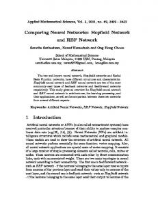
Fig. 1. HNN super-resolution mapping using the Pan mages
dependence assumption. It is, therefore, suggested that the information at higher spatial resolution could be used to increase the detail and accuracy of the resulted sub-pixel land cover map of super-resolution mapping [20]. Several remote sensing systems provide both multispectral (MS) and PAN images such as SPOT 5 with 10 m MS and 5 m PAN imagery, Ikonos 4 m MS and 1 m PAN imagery or QuickBird 2.6 m MS and 0.6 m PAN imagery. In the same remote sensing system, the MS images are usually in lower spatial resolution but higher spectral resolution. For land cover classification, the MS imagery was used because of its high spectral resolution. The PAN imagery, althought with higher spatial resolution, was rarely used for land cover classification since its low spectral resolution. However, for super-resolution mapping, the high spatial resolution PAN image can provide useful information for producing more detailed and accurate sub-pixel land cover maps.
2. Method The new method proposed in this paper aims to use a PAN image as additional information for super-resolution mapping. To make use of the PAN image for land cover mapping, a forward model, a spectral convolution model and an inverse model were employed in the form of a panchromatic reflectance constraint. The panchromatic reflectance constraint was obtained using an minimum grey value difference methods. Fig. 1 is a graphical depiction of the method proposed for incorporating a Pan image into the super-resolution mapping using HNN. From the MS images at the original spatial resolution the land cover area proportion images are produced by a soft-classification procedure. The area proportion images are then used to constrain the HNN to produce the superresolution land cover map in the first iteration of the optimization process. From the super-resolution map at the first iteration, an estimated MS image (at the PAN image spatial resolution) is then produced using a forward model. The estimated MS image is then convolved spectrally to create a synthetic Pan image. An error image is then produced by comparison of the observed and synthetic PAN images. For all neurons covered by the same pixel in the PAN image, a value is produced to adjust the estimated MS image. Thus, the HNN is constrained by the grey values of the Pan image. The adjustment value, or panchromatic reflectance constraint value, along with the goal and constraint values in the HNN structure proposed by Tatem et al. [14], can be used in the optimisation process for super-resolution mapping by minimising the energy function. After the optimisation process, the estimated grey value of the synthetic PAN image produced from sub-pixels in the super-resolution land cover map should be very similar to the observed PAN image. The method presented is based on the structure of the HNN proposed by Tatem et al. [14]. The structure of the HNN for super-resolution mapping of two land cover classes can be seen in Fig. 2. A pixel at the original spatial resolution is divided into two inter-connected matrices of neurons in the HNN. Each neuron (h,i,j) represents a sub-pixel at position (i,j) in the land cover class h and each matrix of neurons represents a land cover class. The HNN is a recurrent neural network and it reaches a stable state when the energy function is minimised. For super-resolution mapping, the HNN is initialised using the soft-classified land cover proportions and runs until it converges to a monotonic stable state. At the stable state, the output values of the neurons are binary values. If the output value of the neuron (h,i,j) is 1, the sub-pixel (i,j) is assigned to the land cover class h. Otherwise, if the output value is 0, the sub-pixel (i,j) does not belong to the class h. The energy function can be expressed as
(i=mf+f-1, j=nf+f-1)
Class 1: 60% Class 2: 40%
A pixel at original level
(m,n)
HNN neuron layer of class 1
Connection between two layers
(i=mf, j=nf)
Corresponding four HNN neuron layer of class 2 pixels of the Pan image Fig. 2. Panchromatic reflectance constraint for sub-pixels covered by pixel (m,n) at the Pan spatial resolution. A pixel at the original level contains four pixels at the Pan image resolution. m, n are the coordinates of the Pan pixel. The panchromatic reflectance constraint ensures that the grey value of the pixel (m,n) of the synthetic Pan image estimated from the neuron output is as close as possible to the grey value of corresponding pixel of the observed Pan image.
E = − ∑ ∑ ∑ ( k1G1hij + k2G 2 hij + k3 Phij + k4 M hij ) , h
i
j
(1)
where k1, k2, k3 and k4 are weighting constants. The weighting constants determine the effects of the goal functions G1hij and G2hij, proportion constraint Phij and multi-class constraint Mhij in the energy function. The optimised values of the weighting constants are determined empirically for super-resolution mapping [14]. For each neuron (h,i,j), the values of spatial clustering or goal functions G1hij and G2hij can be determined by ⎛ ⎛ i +1 j +1 ⎞ ⎞ dG1hij 1 ⎜ 1 (2) = ⎜ 1 + tanh ⎜ ∑ ∑ vhde − 0.5 ⎟ λ ⎟⎟ ( vij − 1) ⎜⎜ 8 d = i −1 e = j −1 ⎟⎟ ⎟ dvhij 2⎜ d i e j ≠ ≠ ⎝ ⎠ ⎠ ⎝ and ⎛ ⎛ ⎛ i +1 j +1 ⎞ ⎞⎞ dG 2 hij 1 ⎜ ⎜ 1 ⎟ ⎜ (3) = ⎜ 1 + ⎜ − tanh ∑ vhde ⎟⎟ λ ⎟⎟ ⎟ ( vij ) , ⎜⎜ 8 d ∑ dvhij 2⎜ ⎜ = i −1 e = i −1 ⎟ ⎟ ⎟ ⎝ d ≠i e ≠ j ⎠ ⎠⎠ ⎝ ⎝ where λ is the gain that is usually assigned a value of 100, 0.5 is the threshold for a neuron to be a sub-pixel of the land cover class h, and 1/8≡1/N where N is the number of neighbouring sub-pixels used in the goal function. The first goal function (Equation 2) is used to increase the output value vhij of the neuron if the average output value of the surrounding neurons is greater than 0.5. In contrast, the second goal function (Equation 3) decreases vhij if the average output value of the surrounding neurons is less than 0.5. The proportion constraint value Phij in Equation 1 retains the land cover proportion for each original pixel and is defined as dPhij 1 xz + z −1 yz + z −1 (4) = 2 ∑ ∑ (1 + tanh ( vhde − 0.5 ) λ ) − a xy , dvhij 2 z d = xz e = yz 1 xz + z −1 yz + z −1 ∑ ∑ (1 + tanh ( vhde − 0.5 ) λ ) 2 z 2 d = xz e = yz is the estimated proportion and axy is the input proportion of the land cover h of the pixel (x,y) which is obtained by soft classification. The pixel (x,y) is the corresponding pixel at the original spatial resolution of the sub-pixel or neuron (h,i,j). z is the zoom factor, which determines the increase in spatial resolution from the original image to the super-resolution mapping image. The proportion constraint function contributes a positive value if the estimated proportion of the class h is greater than the input proportion. As a result, the network reduces the output values of neurons in the class layer h. Conversely, if the estimated proportion is less than the input proportion, the proportion constraint produces a negative value to increase the output values of the neurons in the class h.
where
The multi-class value Mhij is used to reduce the output of the neurons if the sum of outputs of c classes at the position (i,j) is higher than 1. If the sum of outputs of c classes is less than 1, the function increases the output of the neurons at the position (i,j). The value of the multi-class constraint is calculated as dM hij dvhij
⎛ c ⎞ = ⎜ ∑ vkij ⎟ − 1 . ⎝ k =0 ⎠
(5)
To use the PAN image for super-resolution mapping by the HNN, the energy function in Equation 1 is modified by adding a panchromatic reflectance constraint. In this experiment, a function based on the grey value of the PAN image is added to the goal functions and proportion constraint that comprise the energy function. The new energy function can be expressed in an equation as follows (6) E = − ∑ ∑ ∑ ( k1G1hij + k2 G 2 hij + k3 Phij + k4 M hij + k5 RhijP ) , h
P hij
where R
i
j
is the panchromatic reflectance constraint value for each neuron (h,i,j).
The structure of the modified HNN can be seen in Fig. 3. Each neuron in the HNN represents a sub-pixel point in the original spatial resolution image. The fusion factor f determines the increase in spatial resolution of the new superresolution image in comparison with the PAN image. Apart from the proportion constraint for each original pixel, f×f sub-pixels covered by pixel (m,n) of the PAN images are constrained by a panchromatic reflectance constraint. The reflectance constraint is based on the principle that the average estimated grey value from all sub-pixels located within a pixel of the PAN image should be equal to the observed grey value (or target reflectance) of that pixel. For each band of the PAN image, there is an additional constraint for the energy function. The energy function is minimised if the derivatives of variables in Equation 6 converge to 0 for each neuron (h,i,j), dEhij dG1hij dG 2 hij dPhij dM hij dRhij = k1 + k2 + k3 + k4 + k5 . (7) dvhij dvhij dvhij dvhij dvhij dvhij The derivative values of G1, G2, P, and M with respect to vhij are computed by Equation 2, 3, 4 and 5, respectively. To derive the value dRhij/dvhij, every procedure in the diagram in Fig. 2 must be determined. Forward model: The forward model is used to estimate a set of multispectral bands from a land cover image. The estimated reflectance of the neurons representing the pixel (m,n) of 3 multispectral bands at the panchromatic spatial resolution can be defined by a forward model as RBt 1 = sB1,1VC1 + ... + sB1,cVCc (8) RBt 2 = sB 2,1VC 2 + ... + sB 2,cVCc or R t = SV t , RBt 3 = sB 3,1VC1 + ... + sB 3,cVCc mf + f −1 nf + f −1
where the estimated proportion value of a class Ci at the time t is VCit = 1/ f 2 ( ∑
p =mf
∑ vipq ) , sBiCj is the spectral value of
q =nf
the land cover class j for a spectral band Bi, R tm ,n = [ RBt 1 RBt 2 .. RBbt ]Tmn , Vmnt = [VCt1 VCt 2 .. VCt 3 ]Tmn and ⎡ sB1C1 ... sB1Cc ⎤ ⎢ ⎥ S = ⎢ sB 2C1 ... sB 2Cc ⎥ . (9) ⎢s ⎥ ⎣ BbC1 ... sBbCc ⎦ Spectral convolution: The spectral convolution procedure is employed to create a synthetic panchromatic image from a set of multispectral bands. Spectral convolution can be based on the synthesising method proposed by Zhang [21] as (10) RPan = ∑ϕi RBi ,
where RPan is the digital value of the synthetic panchromatic image, RBi is the reflectance value of the multispectral band i, and φi is a weighting factor for the multispectral band i. The weight factor φi can be calculated directly from the panchromatic and multispectral images using multiple regressions of the original panchromatic image and the original multispectral bands. Error image: From the observed panchromatic image, it is possible to produce an error image that can be used for HNN super-resolution mapping. The error image is the difference between the observed panchromatic image and the synthetic panchromatic image created by the neuron output of the HNN at the time t. The error image can be calculated as , (11) E = R o − Rt PanSyn
where Rt is the synthetic panchromatic image at the time t, which can be calculated by the spectral convolution PanSyn model as in the Equation 10 as
t t . RPanSyn = ∑ϕi RBi
(12)
Inverse model and panchromatic reflectance constraint: From the error image, an output value for each neuron in the HNN can be produced based on an inverse model. This output value can be named as panchromatic reflectance constraint, which is used to retain the grey value of each pixel of the panchromatic image. If the grey value of a synthesised panchromatic pixel is greater than that of the corresponding observed panchromatic pixel, the constraint produces a value to reduce the grey of the synthetic image. Conversely, if the synthetic reflectance value of a panchromatic pixel is smaller than that of the observed panchromatic image, the constraint produces a value to increase the grey value of the synthetic image. Supposing that the multispectral bands at spatial resolution of PAN image are B1, B2,.., Bb and the estimated land cover proportions of c land cover classes for pixel (m,n) such as P1, P2,.., Pc. Using the forward model in Equation 8, the relationship between the reflectance of the multispectral bands and the land cover classes can be expressed as RBo1 = sB1,1 P1 + ... + sB1,c Pc RBo 2 = sB 2,1 P1 + ... + sB 2,c Pc or R omn = SPmn , RBo 3 = sBb ,1 P1 + ... + sBb ,c Pc where
R mn = [ RB1 .. RBi .. RBb ]Tmn ,
(13)
is the vector of reflectance values of the bands B1,..,Bi,..,Bb and
Pc ]Tmn
Pmn = [ P1 P2 .. is the vector of land cover proportion values. In sub-pixel mapping, based on the assumption that a pixel consists of a matrix of crisp sub-pixels, the land cover proportions P1, P2,.., Pc must be whole number of subpixels. For example, if a pixel in the PAN image consists of 2x2 sub-pixels, the land cover proportion of a land cover class Pi should be the integer values such as 0, 1, 2, 3 and 4. The land cover proportions of all c land cover classes of a pixel in the PAN image are combination of the integer values such as P1=1/4, .., Pi=0,.., Pc=3/4 with P1 + P2 + ..+Pc = 1. The synthetic grey value of a PAN pixel would converge to the observed grey value if the estimated proportion value VCit of class c at the time t is equal to the land cover proportion Pi or the error image would converge to zero. The land cover class proportions or the proportion combination of land cover classes for each PAN pixel can be determined from a limited number of possible combinations of land cover class. For example, land cover proportions of a PAN pixel (m,n) which contains two land cover classes P1 and P2 can be one of the possible combinations (provided that a pixel in the Pan image cover 2x2 sub-pixels) such as [P1=0, P2=1], [P1=1/4, P2=3/4], [P1=2/4, P2=2/4], [P1=3/4, P2=1/4], and [P1=1, P2=0]. In this research, the land cover proportion combination of a PAN pixel can be determined base on minimum grey value difference method. The minimum grey value difference method is based on the forward model (Equations 8) and spectral convolution (Equation 10). To calculate the land cover proportions for pixel (m,n) in the PAN image, the difference between the synthetic grey value computed from each possible land cover proportion combination and the observed grey value is calculated. The land cover proportion combination of the pixel can be chosen based on the minimum difference. The process can be expressed by a rule as follows: (14) P = Pi if ( RiSynthetic − R Observed mn = min )
where P is vector of land cover proportion for PAN pixel (m,n), Pi is vector of the land cover proportion combination number i, RiSynthetic is synthetic grey value from the land cover proportion combination number i, and R Observed is grey value of the observed PAN image. When the land cover proportion image P is obtained, the panchromatic reflectance function value can be calculated as t dR / dvhij = Phmn − Vhmn (15) t where (m,n) is corresponding pixel of the pixel (i,j) in the PAN image, Phmn is land cover proportion of class h and Vhmn is estimated land cover proportion of class h of the pixel (m,n) at the time t.
3. Data In this experiment, a simulated 32 m MS image and a 8 m PAN spectral image based on a real IKONOS image was used. The ratio between the spatial resolution of the simulated MS and PAN image is similar to the ratio between the real 4 m MS and 1 m panchromatic IKONOS image. Thus, the algorithm can be applied for the real image (e.g. 4 m MS and 1 m PAN image which is obtained from 4 m MS and 1 m PAN image) if it performs successfully on the simulated image. The simulation ensured that there were no errors in image registration between the reference image and the land cover image obtained by super-resolution mapping. Therefore, the evaluation of the performance of the algorithm was more precise. The experiment was implemented in four steps as follows: (1)- Raw data analysis, (2)- Data simulation, (3)- Preprocessing, and (4)- Super-resolution mapping (Fig. 3).
(a) (b) (c) (d) Fig. 4. (a) Land cover map at 4 m spatial resolution used for simulating data, (b) 4 m cereal class map, (c) 4 m grass class map, (d) 4 m trees class map.
1) Raw data analysis Raw data: An IKONOS MS image was acquired over an area of Eastleigh, Southampton, UK. The IKONOS image consisted of four 4 m MS bands in the following wavebands: Red (632-698 nm), Near-Infra Red (NIR: 757-853 nm), Green (506-595 nm) and Blue (445-516 nm) and a 1 m PAN band (450-900 nm). Reference data and statistical information: The experiment was implemented in an area of 64×64 pixels (at 4 m spatial resolution level) that consists of three land cover classes: cereal, grass, and trees (Fig. 4(a), 4(b), 4(c) and 4(d). These three land cover classes were produced using maximum likelihood classification of the real IKONOS image. Statistical information such as the means and standard deviations of the three land cover classes in the area was obtained. These three land cover classes were used as a reference for sub-pixel map obtained by the proposed algorithm.
2) Data simulation Multispectral imagery (8 m): From the land cover map (Fig. 4(b), 4(c), 4(d)) at 4 m spatial resolution, a set of multispectral images at 4 m spatial resolution was simulated based on the random normal distribution and the mean and variance of each land cover obtained by real data analysis. The simulated MS image therefore is similar to an IKONOS image at 4 m spatial resolution. An MS image at 8 m spatial resolution was generated by degrading the 4 m simulated MS image by a factor of two (Fig. 6(a), 6(b), 6(c), 6(d)). Panchromatic imagery (8 m): . The 8 m simulated MS image was then used to create a simulated PAN image (Fig. 6(e)) based on a simple spectral convolution of the Blue, Green, Red and NIR bands of the 8 m simulated MS image (the wavelength of the PAN band of the IKONOS image covers these four bands) as Pan =
BLUE + GREEN + RED + NIR . 4
(16)
Multispectral imagery (32 m): The 32 m MS image (Fig. 6(f), 6(g), 6(h), 6(i)) was produced by degrading the 4 m MS image by a factor of eight. The 32 m MS image was then used for soft-classification to produce a 32 m land cover proportion image and a 8 m PAN image.
3) Pre-processing To provide a more realistic test, a set of proportion images was produced using soft-classification of the simulated 32 m MS image. The simulated (rather than real) MS image was used because the three land cover classes at the subpixel (4 m) level are known, facilitating direct evaluation of the technique. A k-nearest neighbour classifier (k-NN) [5] was used for soft-classification with k=5. The land cover proportion image was produced with overall area error proportion of 0.005552 and overall RMS error of 0.083775 [13]. Statistics for the resulting land cover map from soft-classification show that the land cover proportion images contained an amount of error similar to that of a soft-classified real MS image. In this sense, the simulated land cover proportion image was similar to that might be obtained from the real data.
4) Local end-member spectra Three land cover classes exhibited a large variance over all four spectral bands (Fig. 5). Thus, a single set of endmember spectra values used in Equation 2 was not appropriate for every pixel in the image. Investigation of the real IKONOS image indicated that the digital numbers of adjacent pixels of the same class are similar. Hence, it is suggested that using locally defined end-member spectra would be more appropriate for determining the local reflectance constraint value than using a single value for the whole image.
(a)
(b)
(c)
Fig. 5. Histrogram of three classes in four bands of IKONOS MS image; Dot line-Band 1; Dash line-Band 2; Dot and dash line-Band 3; Solid line-Band 4.
(a)
(b)
(c)
(d)
(e)
(f)
(g)
(h)
(i) (k) (l) (m) Fig. 6. Four bands (a) Red, (b) NIR, (c) Green, and (d) Blue 8 m of simulated MS IKONOS image. (e) 8 m simulated PAN image. Four bands (f) Red, (g) NIR, (h) Green, and (i) Blue of 32 m simulated image. Three bands (k) Red, (l) Green, and (m) Blue of 8 m simulation of the PAN MS image.
The local end-member spectra can be produced from the land cover proportion image and the original MS image (e.g., 32 m land cover proportion image and 32 m MS image). Fig. 8 describes the local end-member spectra calculation process. The end-member spectra values of the pixel (m,n) in the 8 m PAN image of a given MS band can be defined based on the class proportions and the reflectance value of the corresponding pixel (x,y) and its eight surrounding pixels of the same MS band of the 32 m MS image. For each spectral band and each pixel (x,y), an equation exists as follows RBixy = SBiC1PCxy1 + SBiC 2 PCxyj2 + ... + SCc PCcxy , (17) where RBixy is the digital number of pixel (x,y) in spectral band Bi, PCxy1 , PCxy2 ,..., PCcxy are class proportions and SBiC1, SBiC2,.., SBiCc are the local end-member spectra of the pixel (x,y) in spectral band Bi. With eight surrounding pixels, there are eight equations which can be rewritten in matrix form as xy R Bi = PS Bi , xy Bi
(18) ( x −1)( y −1) Bi
where R = [ R
( x+1)( y +1) T Bi
... R
] ,S
xy Bi
= [ S BiC1 ... S BiCc ] , and
70
70
91
90
92
110
89
90
110
(m, n)
(x=(int)m/f, y=(int)m/f) 70% grass 30% trees
70% grass 30% trees
50% grass 50% trees
50% grass 50% trees
51% grass 49% trees
30% grass 70% trees
51% grass 49% trees
51% grass 49% trees
30% grass 70% trees
Fig. 7. Local end-member spectra calculation: (m,n) are coordinates of the PAN image pixel and (x,y) are coordinates of the pixel in the original image that corresponds to the PAN pixel (m,n). From land cover proportion and digital number of pixel (x,y) and its eight surrounding pixels, the local spectra of the pixel (m,n) can be calculated.
⎡ PC(1x−1)( y −1) ⎢ .. ⎢ ⎢ P= PCxy1 ⎢ .. ⎢ ⎢ ( x+1)( y +1) ⎣ PC1
.. PCc( x−1)( y −1) ⎤ ⎥ .. .. ⎥ .. PCcxy ⎥ ⎥ .. .. ⎥ ⎥ .. PCc( x+1)( y +1) ⎦
. Using the least squares method, the local end-member spectra SBi can be resolved as
(
S Bi = PT P
)
−1
PT R Bi .
(19)
Amongst the pixels that are used to determine the local end-member spectra, the pixel (x,y) should be the most important since it covers the PAN pixel (m,n). To emphasise the contribution of the corresponding pixel (x,y) to the endmember spectra, a weight mechanism was used such that Equation 19 becomes
(
S Bi = PT WP
)
−1
WPT R Bi ,
(20)
where W was the diagonal matrix: ⎡ w( x−1)( y −1) ⎢ 0 ⎢ W=⎢ 0 ⎢ 0 ⎢ ⎢ 0 ⎣ (x-1)(y-1)
xy
0
0
..
0
0 0
0 wxy
0
0
0
..
0
0
0
⎤ ⎥ 0 ⎥ ⎥ 0 ⎥ 0 ⎥ ⎥ w( x+1)( y +1) ⎦ 0
(21)
(x+1)(y+1)
and w ,..,w ,.., w are weight values for each corresponding pixel. The optimal weight value wxy was tested xy using the weight value w of 1 up to 20 and the other weight values of 1.
4. Results Two sources of data were used in the HNN super-resolution mapping using the PAN imagery. The first data source was the land cover proportion image obtained by soft-classification. The second data source is the PAN image. From the real soft-classified land cover proportion image (Fig. 8(a), 8(b), and 8(c)), the 4 m sub-pixel land cover maps were obtained using the traditional HNN (Fig. 8(g), 8(h), and 8(i)), and the HNN using the PAN image with local end-member spectra (Fig. 8(j), 8(k) and 8(l)). The greatest accuracy land cover map was obtained with the weighting coefficients of k1=70, k2=70, k3=70, k4=70 and k5=70 after 6000 iterations with the optimal weight for determining local end-member spectra of 14. The 32 m hard classified land cover image (Fig. 8(d), 8(e) and 8(f)) was produced from the 32 m
(a)
(d)
(g)
(j)
(b)
(e)
(h)
(k)
(l) (c) (f) (i) Fig. 8. 4 m Cereal (a) , Grass (b) , and Trees (c) land cover proportion image. 4 m Cereal (d), Grass (e), Trees (f) hard classified land cover image. 4 m Cereal (g) , Grass (h), Trees (i) HNN super-resolution mapping image. : 4 m Cereal (j), Grass (k), Trees (i) HNN super-resolution mapping using the PAN with the local end-member spectra resulting image.
multispectral image (Fig. 6(g), 6(h), 6(i), and 6(k)) using a neural network classification. Accuracy statistics for each class based on KIA, overall accuracy, and per-class omission and commission errors are presented in Table 1. to evaluate the predicted sub-pixel spatial resolution map. Visual comparison of the results of the new techniques shows that the super-resolution mapping using the PAN image is clearly preferable to hard classification and the traditional HNN super-resolution mapping technique. The improvement of the technique is most obviously seen in the trees class, where most of the trees objects are smaller than the 32 m simulated image pixel. Without information from the PAN image, the trees class sub-pixels of the linear objects in the right-bottom and in the top of Fig. 4(d) were clustered into larger objects to satisfy the goal functions as in Fig. 8(i). The panchromatic reflectance constraint produced a value to retain reflectance for the neurons in those linear objects. Therefore, objects smaller than an original pixel can be mapped (Fig. 8(l), 8(o)). The accuracy evaluation of the HNN super-resolution mapping using the PAN image, the hard classification and the HNN super-resolution mapping used by Tatem et al. [14] are in Table 1. The accuracy statistics shows a considerable increase in accuracy with the new technique. Overall accuracy of the land cover map increased by around 5% from 86.52% for the hard classification to 91.02% for the super-resolution mapping using the PAN image with spectra. The KIA value - κ increased from 0.7533 for the hard classified map to 0.8361 for the new HNN super-resolution mapping. In comparison with the HNN super-resolution mapping without using the PAN image, the accuracy of the thematic map produced by the HNN super-resolution mapping using the PAN image increased 3.5% in terms of overall accuracy. Amongst the three land cover classes, the accuracy of the trees land cover class increased most with the omission error reduced from 56.26% for the hard classified image and 36.82% for the traditional HNN super-resolution mapping to approximately 25% for the new HNN super-resolution mapping technique. Similarly, the commission error reduced from 26.25% and 20.69% to 17.67% after using the PAN image. In the other two classes, the increase in accuracy was not as great as that of the trees class since most sub-pixels in these two classes were grouped into objects larger than a 32 m pixel. However, the increasing values are relatively large if the low omission and commission errors are taken into account. This can be explained by the fact that the clustering goal functions are suitable for large features, yet the detailed information at the fused spatial resolution is essential for more accurate super-resolution mapping of the boundary pixels.
Table 1. Accuracy statistics. Statistics for the hard classified image Unclassified Cereal Grass Trees KIA – κ =
Cereal 0 1005 39 0
Grass 0 126 2305 86 0.7430
Tree 0 21 280 234
ErrorO (%)
ErrorC (%)
3.74 12.76 8.42 12.16 56.26 26.88 Overall accuracy = 86.52%
Statistics for the HNN super-resolution mapping without using the PAN image Unclassified Cereal Grass Trees KIA – κ =
Cereal 0 977 63 4
Grass 4 89 2350 74 0.7814
Tree 3 2 231 299
ErrorO (%) 4.60 8.14 36.82 Overall accuracy
ErrorC (%) 1.000 8.52 11.12 20.69 88.53%
Statistics for the HNN super-resolution mapping without using the PAN image Unclassified Cereal Grass Trees KIA – κ =
Cereal 10 983 34 17
Grass 70 30 2349 68 0.8361
Tree 31 2 106 396
ErrorO (%) 5.84 6.67 25.98 Overall accuracy
ErrorC (%) 1.000 3.15 5.62 17.67 91.02%
The number of unclassified pixels (Table 1) was slightly increased in the super-resolved land cover image using the PAN image in comparison with the results of the traditional HNN super-resolution mapping. These unclassified subpixels occurred as the goal functions, proportion constraint and multi-class constraint could not be satisfied simultaneously. However, the number of unclassified pixels did not reduce the accuracy of the new technique.
3. Conclusions This paper introduces the use of PAN images for super-resolution mapping. Data from the PAN image were incorporated into the HNN optimisation using forward and inverse models in the form of the panchromatic reflectance constraint. The value of the constraint is calculated based on a linear mixture model, which uses local end-member spectra. The effectiveness of the technique was examined using a 32 m land cover proportions image obtained by application of a soft classifier to simulated MS imagery. The proportions images were supplemented by 8 m simulated PAN image. The accuracy evaluation was implemented based on the KIA, overall accuracy, and omission and commission errors. The results demonstrated that PAN images can be used as a source of supplementary information for the HNN to predict accurately land cover at sub-pixel spatial resolution from land cover proportion images. The analysis demonstrated a considerable increase in accuracy with the new technique, particularly for land cover features at the subpixel scale. For larger features, the technique increases the accuracy slightly. In addition, visual inspection of the resulting image showed pleasing improvements. The result of the experiment suggests the potential for using the panchromatic image in super-resolution mapping processes for the real data.
References [1] J. B. Campell, Introduction to Remote Sensing, Second edition. London: Taylor & Francis, 1996. [2] R. A. Schowengerdt, Remote Sensing: Models and Methods for Image Processing, San Diego: Academic Press, 1997. [3] J. J. Settle and N. A. Drake, “Linear mixing and the estimation of ground cover proportions”, International Journal of Remote Sensing, vol. 14, pp. 1159-1177, 1993. [4] L. Bastin, “Comparison of fuzzy c-means classification, linear mixture modelling and MLC probabilities as tools for unmixing coarse pixels”, International Journal of Remote Sensing, vol. 18, pp. 3629-3648, 1997. [5] R. A. Schowengerdt, “On the estimation of spatial-spectral mixing with classifier likelihood functions”, Pattern Recognition Letters, vol. 17, no. 13, pp. 1379-1387, 1996.
[6] G. M. Foody, R. M. Lucas, P. J. Curran and M. Honzak, “Non-linear mixture modelling without end-members using an artificial neural network”, International Journal of Remote Sensing, vol. 18, no. 4, pp. 937-953, 1997. [7] G. M. Carpenter, S. Gopal, S. Macomber, S. Martens, and C. E. Woodcock, “A neural network method for mixture estimation for vegetation mapping”, Remote Sensing of Environment, vol. 70, pp. 138-152, 1999. [8] M. Brown, H. Lewis and S. Gunn, “Linear spectral mixture models and Support Vector Machines for Remote Sensing”, IEEE Transactions on Geoscience and Remote Sensing, vol. 38, no. 5, pp. 2346-2360, 2000. [9] P. M. Atkinson, “Mapping sub-pixel boundaries from remotely sensed images”, Innovation in GIS 4, pp. 166-180, 1997. [10] P. Aplin and P.M. Atkinson, “Sub-pixel land cover mapping for per-field classification”, International Journal of Remote Sensing, vol. 22, pp. 2853-2858, 2001. [11] J. Verhoeye and R. De Wulf, “Land cover mapping at sub-pixel scales using linear optimisation techniques”, Remote Sensing of Environment, vol. 79, no. 1, pp. 96-104, 2002. [12] A. J. Tatem, H. G. Lewis, P. M. Atkinson and M. S. Nixon, “Super-resolution target identification from remotely sensed images using a Hopfield neural network”, IEEE Transactions on Geoscience and Remote Sensing, vol. 39, no. 4, pp. 781-796, 2001. [13] —, “Multi-class land cover mapping at the sub-pixel scale using a Hopfield neural network”, International Journal of Applied Earth Observation and Geoinformation, vol. 3, no. 2, pp. 184-190, 2001. [14] —, “Super-resolution land cover pattern prediction using a Hopfield neural network”, in G. M. Foody and P. M. Atkinson (eds), Uncertainty in Remote Sensing and GIS, Chichester: John Wiley & Sons, pp. 59-76, 2002. [15] —, “Super-resolution land cover pattern prediction using a Hopfield neural network”, Remote Sensing of Environment, vol. 79, no. 1, pp. 1-14, 2002. [16] A. J. Tatem, “Super-resolution land cover mapping from remotely sensed imagery using a Hopfield neural network”, University of Southampton: Unpublished Ph.D. Thesis., 2002. [17] P. M. Atkinson, “Super-resolution land cover classification using geostatistical optimization”, Edited by X. Sanchez-Villa, GeoENV IV: Geostatistics for Environmental Applications, Kruwer-Dordrecht, 2003. [18] K. C. Mertens, L. P. C. Verbeke, E. I. Ducheyne, and R. R. De Wulf, “Using genetic algorithms in sub-pixel mapping”, International Journal of Remote Sensing, vol. 24, no. 21, pp. 4241 - 4247, 2003. [19] K. C. Mertens, L. P. C. Verbeke, T. Westra and R. R. De Wulf, “Sub-pixel mapping and sub-pixel sharpening using neural network predicted wavelet coefficients”, Remote Sensing of Environment, vol. 91, no. 2, pp. 225-236, 2004. [20] Q. M. Nguyen, P. M. Atkinson and H. G. Lewis, “Super-resolution mapping using Hopfield neural netwok with LIDAR data”, IEEE Geoscience and Remote Sensing Letters, vol. 2, no. 3, pp. 366-370, 2005. [21] Y. Zhang, “A new merging method and its spectral and spatial effects”, Photogrammetric Engineering and Remote Sensing, vol. 20, no. 10, pp. 2003-2014, 1999.