Some of our calculations were performed using the QuTiP simulation package28. This work was supported in part by the Scientific Research (S) Grant No.
Superconducting qubit-oscillator circuit beyond the ultrastrong-coupling regime Fumiki Yoshihara,∗ Tomoko Fuse,† and Kouichi Semba‡ National Institute of Information and Communications Technology, 4-2-1, Nukuikitamachi, Koganei, Tokyo 184-8795, Japan Sahel Ashhab§ Qatar Environment and Energy Research Institute, Hamad Bin Khalifa University, Qatar Foundation, Doha, Qatar Kosuke Kakuyanagi and Shiro Saito NTT Basic Research Laboratories, NTT Corporation, 3-1 Morinosato-Wakamiya, Atsugi, Kanagawa 243-0198, Japan
Abstract The interaction between an atom and the electromagnetic field inside a cavity1–6 has played a crucial role in the historical development of our understanding of light-matter interaction and is a central part of various quantum technologies, such as lasers and many quantum computing architectures. The emergence of superconducting qubits7,8 has allowed the realization of strong9,10 and ultrastrong11–13 coupling between artificial atoms and cavities. If the coupling strength g becomes as large as the atomic and cavity frequencies (∆ and ωo respectively), the energy eigenstates including the ground state are predicted to be highly entangled14 . This qualitatively new regime can be called the deep strong-coupling regime15 , and there has been an ongoing debate16–18 over whether it is fundamentally possible to realize this regime in realistic physical systems. By inductively coupling a flux qubit and an LC oscillator via Josephson junctions, we have realized circuits with g/ωo ranging from 0.72 to 1.34 and g/∆ � 1. Using spectroscopy measurements, we have observed unconventional transition spectra, with patterns resembling masquerade masks, that are characteristic of this new regime. Our results provide a basis for ground-state-based entangledpair generation and open a new direction of research on strongly correlated light-matter states in circuit-quantum electrodynamics.
1
a
c Izpf
C
Ip
2 μm
L0
Φq
ωp Lc GND
GND
b
C
L0
50 μm
FIG. 1. Superconducting qubit-oscillator circuit. a, Circuit diagram. A superconducting flux qubit (red and black) and a superconducting LC oscillator (blue and black) are inductively coupled to each other by sharing a tunable inductance (black). b, Laser microscope image of the lumped-element LC oscillator inductively coupled to a coplanar transmission line. c, Scanning electron microscope image of the qubit and the coupler junctions located at the red rectangle in image b. The coupler, consisting of four parallel Josephson junctions, is tunable via the magnetic flux bias through its loops (see Supplementary Information, sections S1 and S2, and Fig. S1).
We begin by describing the Hamiltonian of each component in the qubit-oscillator circuit, which comprises a superconducting flux qubit and an LC oscillator inductively coupled to each other by sharing a tunable inductance Lc , as shown in the circuit diagram in Fig. 1a. The Hamiltonian of the flux qubit can be written in the basis of two states with persistent currents flowing in opposite directions around the qubit loop19 , |Liq and |Riq , as Hq = −~(∆σx + εσz )/2, where ~∆ and ~ε = 2Ip Φ0 (nφq − nφq0 ) are the tunnel splitting and the energy bias between |Liq and |Riq , Ip is the maximum persistent current, and σx, z are Pauli matrices. Here, nφq is the normalized flux bias through the qubit loop in units of the superconducting flux quantum, Φ0 = h/2e, and nφq0 = 0.5 + kq , where kq is the integer 2
that minimizes |nφq − nφq0 |. The macroscopic nature of the persistent-current states enables strong coupling to other circuit elements. Another important feature of the flux qubit is its strong anharmonicity: the two lowest energy levels are well isolated from the higher levels. The Hamiltonian of the LC oscillator can be written as Ho = ~ωo (ˆ a† a ˆ + 1/2), where p ωo = 1/ (L0 + Lqc )C is the resonance frequency, L0 is the inductance of the superconducting lead, Lqc (' Lc ) is the inductance across the qubit and coupler (see Supplementary Information, section S2), C is the capacitance, and a ˆ (ˆ a† ) is the oscillator’s annihilation (creation) operator. Figure 1b shows a laser microscope image of the lumped-element LC oscillator, where L0 is designed to be as small as possible to maximize the zero-point fluctup ations in the current Izpf = ~ωo /2(L0 + Lqc ) and hence achieve strong coupling to the flux qubit, while C is adjusted so as to achieve a desired value of ωo . The freedom of choosing L0 for large Izpf is one of the advantages of lumped-element LC oscillators over coplanarwaveguide resonators for our experiment. Another advantage is that a lumped-element LC oscillator has only one resonant mode. Together with the strong anharmonicity of the flux qubit, we can expect that our circuit will realize the Rabi model20–23 , which is one of the simplest possible quantum models of qubit-oscillator systems, with no additional energy levels in the range of interest. The coupling Hamiltonian can be written as9 Hc = ~gσz (ˆ a+a ˆ† ), where ~g = M Ip Izpf is the coupling energy and M (' Lc ) is the mutual inductance between the qubit and the LC oscillator. Importantly, a Josephson-junction circuit is used as a large inductive coupler24 (Fig. 1c), which together with the large Ip and Izpf allows us to achieve deep strong coupling. The total Hamiltonian of the circuit is then given by ~ 1 Htotal = − (∆σx + εσz ) + ~ωo (ˆ a† a ˆ + ) + ~gσz (ˆ a+a ˆ† ). 2 2
(1)
Nonlinearities in the coupler circuit lead to higher-order terms in (ˆ a+a ˆ† ). The leading-order term can be written as CA2 ~g(ˆ a+a ˆ† )2 and is known as the A2 term16 in atomic physics. Since this A2 term can be eliminated from Htotal by a variable transformation (see Methods), we do not explicitly keep it and instead use Eq. (1) for our data analysis. Spectroscopy was performed by measuring the transmission spectrum through a coplanar transmission line that is inductively coupled to the LC oscillator (see Supplementary Information, section S3). For a systematic study of the g dependence, five flux bias points in three circuits were used. Circuit II is designed to have larger values of g than the other two, and 3
0.0 6.35
0.5
1.0
01 02
13 24
a
6.34
4.57 GHz 6.33 6.32
b
ωp/2π (GHz)
6.31
4.92 GHz 6.30
c 6.24
6.23 5.79 GHz −20
−10
0
10
20
5.72
5.71
d 7.63 GHz
5.70
−15
−10
−5
0 5 ε/2π (GHz)
10
15
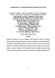
cal are FIG. 2. Transmission spectra for circuits I and II. Calculated transition frequencies ωij
superimposed on the experimental results. As summarized in Table I, panel a shows data from circuit I at nφq = −0.5, panel b shows data from circuit I at nφq = −1.5, panel c shows data from circuit I at nφq = 2.5, and panel d shows data from circuit II at nφq = −0.5. The values of g/2π are written in the panels. The red, green, blue, and cyan lines indicate the transitions |0i → |1i, |0i → |2i, |1i → |3i, and |2i → |4i, respectively.
circuits I and II are designed to have smaller values of ∆ than circuit III. Figures 2a–d show normalized amplitudes of the transmission spectra |S21 (ωp )|/|S21 (ωp )|max from circuits I and II as functions of the flux bias ε and probe frequency ωp (see also Supplementary Information, Figs. S5a-d). Characteristic patterns resembling masquerade masks can be seen around ε = 0. At each value of ε, the spectroscopy data was fitted with Lorentzians to obtain the frequencies ωij of the transitions |ii → |ji, where the indices i and j label the energy eigenstates according to their order in the energy-level ladder, with the index 0 denoting the 4
TABLE I. Set of parameters obtained from fitting spectroscopy measurements. circuit nφq
Figure
√ ∆/2π ωo /2π g/2π α = g/ωo 2g/ ωo ∆ (GHz) (GHz) (GHz)
I
−0.5
2a
0.505 6.336
4.57
0.72
5.1
I
−1.5
2b, 3a
0.430 6.306
4.92
0.78
6.0
I
2.5
2c
0.299 6.233
5.79
0.93
8.5
II
−0.5
2d
0.441 5.711
7.63
1.34
9.6
III
0.5
SI6
3.84
5.63
1.01
2.4
5.588
The parameters are obtained from five sets of spectroscopy data in three circuits. The column “Figure” shows the corresponding figures. “SI” stands for Supplementary Information.
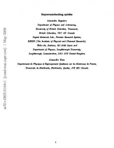
ground state. Theoretical fits to ωij were obtained by diagonalizing Htotal , treating ∆, ωo , and g as fitting parameters. The obtained parameters are shown in Table I. The calculated transition frequencies ωijcal are superimposed on the measured transmission spectra. As g increases, the anticrossing gap between the qubit and the oscillator frequencies at ε ' ±ωo becomes smaller and the signal from the |1i → |3i transition gradually transforms from a W shape to a Λ shape in the range |ε| . ωo . These features are seen in both the experimental data and the theoretical calculations, with good agreement between the data and the calculations. Note that ωo depends on the qubit state and ε via Lqc , which results in the broad V shape seen in the spectra (see Supplementary Information, section S2). To capture signals from more transitions, the transmission spectra in a wider ωp range and a smaller ε range were measured, as shown in Fig. 3a for circuit I at nφq = −1.5. As we approach the symmetry point ε = 0, the signals from the |0i → |2i and |1i → |3i transitions cal disappear while signals from the |0i → |3i and |1i → |2i transitions appear near ω03 and cal ω12 . The appearance and disappearance of the signals are well explained by the transition
matrix elements Tij = hi|(ˆ a+a ˆ† )|ji shown in Fig. 3b: when ε → 0, |T02 | = |T13 | → 0 (forbidden transitions), while |T03 | and |T12 | are maximum (allowed transitions). As can be seen from the expression for Tij , these features are directly related to the form of the energy eigenstates and can therefore serve as indicators of the symmetry properties of the energy 5
eigenstates, similarly to how atomic forbidden transitions are related to the symmetry of atomic wave functions. The weakness of the signals from the |0i → |3i and |1i → |2i transitions is probably due to dephasing caused by flux fluctuations. No signals from the |0i → |3i and |1i → |2i transitions were observed in circuit I at nφq = 2.5 and in circuit II. The broad dips at ωp /2π = 6.2, 6.38, and 6.45 GHz are the result of a background frequency dependence of the transmission line’s transmission amplitude, and these features can be ignored here. The feature at 6.2 GHz also contains a narrow signal from another qubitoscillator circuit that is coupled to the transmission line (see Supplementary Information, section S3). To conclude this analysis of the observed transmission spectra, the fact that the frequencies of the spectral lines and the points where they become forbidden follow, respectively, ωijcal and |Tij | lends strong support to the conclusion that Htotal accurately describes our circuits. Importantly, in circuits II and III, g is larger than both ωo and ∆, emphasizing √ that the circuits are in the deep strong-coupling regime [g & max(ωo , ∆ωo /2)]25 . The fact that at ε = 0 the two forbidden transitions are located between the two allowed transitions is a further sign that g > ωo /2 (see Fig. 3c). In contrast, the highest coupling strengths achieved in previous experiments12,13 give g/ωo = 0.12 and 0.1, respectively. From the spectrum in Fig. 3a, we find that ω01 (ε = 0)/∆ = 0.13 GHz/0.43 GHz= 0.30, meaning that the Lamb shift26 is 70% of the bare qubit frequency. The same value (0.30) is obtained from theoretical calculations for g/ωo = 0.78. Using our experimental results, we can make a statement regarding the A2 term and the superradiance no-go theorem16 in our setup. A direct consequence of the no-go theorem is that, provided that the condition of the theorem (CA2 > g/∆) is satisfied, the system parameters will be renormalized such that the experimentally measured parameters will satisfy √ the inequality 2g/ ∆ωo < 1 (see Methods). However, in all five cases in our experiment, √ we find that 2g/ ∆ωo > 1, with the ratio on the left-hand side ranging from 2.4 to 9.6 (see Table I). These results demonstrate that the A2 term in our setup does not satisfy the condition of the no-go theorem and therefore does not preclude a superradiant state. In fact, we expect that CA2 � 1 as shown in Methods. The energy eigenstates of the qubit-oscillator system can be understood in the following way. In the absence of coupling, the energy eigenstates are product states where the oscillator is described by a Fock state |nio with n plasmons. Because of the coupling to the qubit, 6
6.5
c
6.8
a
6.6 6.4 6.2
6.3
ωij/2π (GHz)
ωp/2π (GHz)
6.4
01 02 03
6.0
4.92 GHz 6.2
5.8 6
|Tij|
1.0 0.5 0.0
12 13
d
4
b
−0.5 0.0 0.5 ε/2π (GHz)
2 0
0
2
4 6 8 g/2π (GHz)
10
FIG. 3. Selection rules and transmission spectrum around the symmetry point. a Transmission spectrum for circuit I at nφq = −1.5 plotted as a function of flux bias ε. The transical superimposed on the experimental result in a and the matrix elements |T | tion frequencies ωij ij
plotted in b are calculated using the parameters shown in Table I, i.e. ∆/2π = 0.430 GHz, ωo /2π = 6.306 GHz, and g/2π = 4.92 GHz. c The calculated transition frequencies around ωo and d from the ground state are plotted as functions of g at ε = 0. The red, green, black, magenta, and blue lines in all four panels indicate the transitions |0i → |1i, |0i → |2i, |0i → |3i, |1i → |2i, and |1i → |3i, respectively. Solid (dashed) lines in panels c and d indicate that the corresponding matrix elements Tij are nonzero (zero). Allowed and forbidden transitions cross at g/2π ' ωo /4π = 3.15 GHz25 , where there is an energy-level crossing and the energy eigenstates |2i and |3i exchange their physical states. The black dotted line is at the coupling strength in circuit I at nφq = −1.5, g/2π = 4.92 GHz.
the state of the oscillator is displaced in one of two opposite directions depending on the ˆ persistent-current state of the qubit25 : |Liq ⊗ |nio → |Liq ⊗ D(−α)|ni o and |Riq ⊗ |nio → ˆ ˆ |Riq ⊗ D(α)|ni a† − α ∗ a ˆ) is the displacement operator, and α is the o . Here, D(α) = exp(αˆ displacement. The amount of the displacement is approximately ±g/ωo . As the energy eigenstates of an isolated qubit at ε = 0 are superpositions of the persistent-current states, √ √ |giq = (|Liq + |Riq )/ 2 and |eiq = (|Liq − |Riq )/ 2, the energy eigenstates of the qubitoscillator system at ε = 0 are well described by Schr¨odinger-cat-like entangled states between 7
TABLE II. The energy eigenstates of the qubit-oscillator system. |qubiti ⊗ |oscillatori basis
energy eigenbasis g
ωo 2
|0i
|0i
|1i
|1i
|2i
|3i
|3i
|2i
arbitrary g
g=0 √
(|Liq ⊗ | − αio + |Riq ⊗ |αio )/ 2 √ (|Liq ⊗ | − αio − |Riq ⊗ |αio )/ 2 √ ˆ ˆ (|Liq ⊗ D(−α)|1i o + |Riq ⊗ D(α)|1io )/ 2 √ ˆ ˆ (|Liq ⊗ D(−α)|1i o − |Riq ⊗ D(α)|1io )/ 2
|giq ⊗ |0io |eiq ⊗ |0io |giq ⊗ |1io |eiq ⊗ |1io
The left two columns are written in the energy eigenbasis while the right two columns are written in the tensor product basis of qubit and oscillator states. At g ' ωo /2, there is an energy-level crossing and the energy eigenstates |2i and |3i exchange their physical states. |Liq and |Riq are the persistentcurrent states of the qubit, |giq and |eiq are the energy eigenstates of the ˆ ˆ qubit, | ± αio = D(±α)|0i o are coherent states of the oscillator, D(α) is a displacement operator, and |nio is a Fock state of the bare oscillator. At g = 0 and hence α = 0, the energy eigenstates are product states, as shown in the right-most column. For arbitrary g, the energy eigenstates of the qubit-oscillator system are entangled states.
ˆ persistent-current states of the qubit and displaced Fock states of the oscillator D(±α)|ni o, ˆ as shown in Table II. Note that the displaced vacuum state D(α)|0i o is the coherent state √ P n |αio = exp(−|α|2 /2) ∞ n=0 α / n!|nio . Although the above picture works best when ωo � ∆, theoretical calculations show that it also gives a rather accurate description for circuit III (with ωo /∆ = 1.44) (see Methods). The vanishing of the spectral lines corresponding to the |0i → |2i and |1i → |3i transitions at ε = 0 is a consequence of the symmetric form of the energy eigenstates. This symmetry is expected from the current-inversion symmetry in the Hamiltonian Htotal , and it supports the theoretical prediction that the energy eigenstates at that point are qubit-oscillator entangled states. Using Htotal and the parameters shown in Table I, we can calculate the qubit-oscillator ground-state entanglement Egs (see Supplementary Information, section S5). In all cases, Egs & 90%, and for circuit II in particular Egs = 99.88%. In comparison, the ground-state 8
entanglement for the parameters of Refs. 12 and 13 is 6% and 4%, respectively. It should be noted here that in all five cases in our experiment there will be a significant population in the state |1i in thermal equilibrium, and the thermal-equilibrium qubit-oscillator entanglement will be reduced to below 8% for circuits I and II, and 25% for circuit III (see Supplementary Information, Table S1). In conclusion, we have experimentally achieved deep-strong coupling between a superconducting flux qubit and an LC oscillator. Our results are consistent with the theoretical prediction that the energy eigenstates are Schr¨odinger-cat-like entangled states between persistent-current states of the qubit and displaced Fock states of the oscillator. We have also observed a huge Lamb shift, 70% of the bare qubit frequency. The tiny Lamb shift in natural atoms, which arises from weak vacuum fluctuations, was one of the earliest phenomena to stimulate the study of quantum electrodynamics. Now we can design artificial systems with light-matter interaction so strong that instead of speaking of vacuum fluctuations we speak of a strongly correlated light-matter ground state, defining a new state of matter and opening prospects for applications in quantum technologies. Note added in proof: After acceptance of our paper, we became aware of a related manuscript (Ref. 27) taking a different approach to the same theme.
ACKNOWLEDGMENTS
We thank Kae Nemoto, Masao Hirokawa, Kunihiro Inomata, John W. Munro, Yuichiro Matsuzaki, Motoaki Bamba, and Norikazu Mizuochi for stimulating discussions. The authors are greatful to Mikio Fujiwara, Kentaro Wakui, Masahiro Takeoka, and Masahide Sasaki for their continued support through all the stages of this research. We thank Junichi Komuro, Shinya Inoue, and Etsuro Sasaki for assistance with experimental setup. We also thank Sander Weinreb for their support by providing excellent cryoamplifiers, and Noriyoshi Matsuura and Yoshitada Kato for their cordial support in the startup phase of this research. Some of our calculations were performed using the QuTiP simulation package28 . This work was supported in part by the Scientific Research (S) Grant No. JP25220601 by the Japanese Society for the Promotion of Science (JSPS). 9
AUTHOR CONTRIBUTIONS
All authors contributed extensively to the work presented in this paper. F. Y., T. F., K. S. carried out measurements and data analysis on the coupled flux qubit - LC-oscillator circuits. F. Y., T. F. designed and F. Y., T. F., K. K. fabricated the flux-qubit and associated devices. T. F., F. Y., K. K., S. S., and K. S. designed and developed the measurement system. S. A. provided theoretical support and analysis. F. Y., T. F., S. A., and K. S. wrote the manuscript, with feedback from all authors. K. S. designed and supervised the project.
METHODS
Laser microscope image. The laser microscope image in Fig. 1b was obtained by Keyence VK-9710 Color 3D Laser Scanning Microscope. The magnification of the objective lens is 10. The application “VK Viewer” was used for image acquisition. Scanning electron microscope image. The scanning electron microscope image in Fig. 1c was obtained by JEOL JIB-4601F. The acceleration voltage was 10 kV, the magnification was 6500, and the working distance was 8.7 mm. Nonlinearity of M and the A2 term of the total Hamiltonian.
We now con-
sider the nonlinearity of the mutual inductance M between the flux qubit and the LC oscillator. As discussed in the Supplementary Information, M is almost the same as Lc in Fig. 1a, which depends on the current flowing through the Josephson junction Ib as p Lc (Ib ) = Φ0 /(2π (ac Ic )2 − Ib2 ), where ac Ic ≡ IcM is the critical current of the Josephson junction. We thus assume that M can similarly be written as
M (Ib ) =
Φ p 0 . 2 2π IcM − Ib2
(2)
The nonlinearity of M (Ib ) up to second order in δIb can be written as
∂M (Ib ) δIb2 ∂ 2 M (Ib ) M (Ib + δIb ) = M (Ib ) + δIb + ∂Ib 2 ∂Ib2 � � 2 Ib δIb IcM + 2Ib2 2 = M (Ib ) 1 + 2 + δI . 2 IcM − Ib2 2(IcM − Ib2 )2 b 10
(3)
The coupling Hamiltonian can be written as Hc = M (Iˆq + Iˆo )Iˆq Iˆo = M (Iˆq + Iˆo )Ip σz Izpf (ˆ a+ a ˆ† ), where Iˆq = Ip σz is the persistent-current operator of the qubit, Iˆo = Izpf (ˆ a+a ˆ† ) is the current operator of the oscillator, and the current Iˆq + Iˆo flows through the mutual inductance. Typically, Ip � Izpf . Taking into account the nonlinearity of M (Iˆq + Iˆo ), the coupling Hamiltonian is written as
Hc = M (Iˆq + Iˆo )Iˆq Iˆo ! 2 IcM + 2Iˆq2 2 = M (Iˆq ) 1 + 2 + Iˆo Iˆq Iˆo 2 IcM − Iˆq2 2(IcM − Iˆq2 )2 � � 2 3 2 + 2Ip2 )Ip Izpf (IcM Ip2 Izpf † 2 † 3 † (ˆ a+a ˆ) + σz (ˆ a+a ˆ) = M (Ip ) Ip Izpf σz (ˆ a+a ˆ )+ 2 2 IcM − Ip2 2(IcM − Ip2 )2 Iˆq Iˆo
= ~g[σz (ˆ a+a ˆ† ) + CA2 (ˆ a+a ˆ† )2 + CA3 σz (ˆ a+a ˆ† )3 ],
(4)
where
~g = M (Ip )Ip Izpf ,
CA2 =
Ip Izpf , 2 IcM − Ip2
(5)
(6)
and
CA3
2 2 (IcM + 2Ip2 )Izpf = . 2 2(IcM − Ip2 )2
(7)
Here, we considerd terms up to second order in Izpf /Ip . We find that 1 � CA2 � CA3 considering the following relation, IcM (= ac Ic ) > Ip (. a3 Ic ) � Izpf (� Ic ), where ac & 1 (see Supplementary Material), 0.4 . a3 . 0.8, Ic is several hundred nano amperes, and Izpf is several ten nano amperes. Since the term CA3 is very small, we ignore the third term in Eq. (4). The total Hamiltonian of the circuit considering the nonlinearity of M up to first order in Izpf /Ip is given by 11
Htotal = − ~2 (∆σx + εσz ) + ~ωo a ˆ† a ˆ+
1 2
�
+ ~gσz (ˆ a+a ˆ† ) + CA2 ~g(ˆ a+a ˆ† )2 ,
(8)
where the first term is the Hamiltonian of the flux qubit, the second term is the Hamiltonian of the LC oscillator, and the third term is the coupling Hamiltonian. The fourth term proportional to (ˆ a+a ˆ† )2 is known as the A2 term in atomic physics. This term can be eliminated by a variable transformation as
Htotal
� � 1 ~ † ˆa ˆ+ + CA2 ~g(ˆ a+a ˆ† )2 + ~gσz (ˆ a+a ˆ† ) = − (∆σx + εσz ) + ~ωo a 2 2 � � ~ ~ωo ~ωo = − (∆σx + εσz ) + + CA2 ~g (ˆ a+a ˆ † )2 − (ˆ a−a ˆ† )2 + ~gσz (ˆ a+a ˆ† ) 2 4 4 0 0 ~ ~ω ~ω = − (∆σx + εσz ) + o (ˆb + ˆb† )2 − o (ˆb − ˆb† )2 + ~g 0 σz (ˆb + ˆb† ) 2 4 4 ~ 1 = − (∆σx + εσz ) + ~ωo0 (ˆb†ˆb + ) + ~g 0 σz (ˆb + ˆb† ), (9) 2 2
where
ωo0 =
p
ωo2 + 4CA2 gωo ,
0
r
g =
ωo g, ωo0
(10)
(11)
and the new field operators, ˆb + ˆb† =
r
ωo0 (ˆ a+a ˆ† ) ωo
(12)
ωo (ˆ a−a ˆ† ), ωo0
(13)
and ˆb − ˆb† =
r
are used. The form of the Hamiltonian in Eq. (9) is exactly the same as the one where the coupling term is linear in (ˆ a+a ˆ† ), which is given by linear Htotal = − ~2 (∆σx + εσz ) + ~ωo (ˆ a† a ˆ + 12 ) + ~gσz (ˆ a+a ˆ† ).
12
(14)
Note that the transformation described by Eqs. (12) and (13) is a Hopfield-Bogoliubov transformation29 . It guarantees that [ˆb, ˆb† ] = [ˆ a, a ˆ† ] = 1. In other words, both the a ˆ operators and the ˆb operators obey the harmonic oscillator commutation relations. The two sets of operators are related to each other by quadrature squeezing operations. The most natural choice among these two and all other quadrature-squeezed variants is the one that leads to the standard form of the harmonic oscillator Hamiltonian, usually expressed as ~ωo a ˆ† a ˆ. As such, the ˆb operators are the most natural oscillator operators for our circuits. The a ˆ operators were defined based on an incomplete description of the circuit, considering the properties of the LC circuit and ignoring the qubit and coupler parts of the circuit. In particular, the A2 term in our circuits describes an additional contribution to the inductive energy of the oscillator that arises in the presence of the qubit and coupler circuits. Similarly, the expression given in the main text for the current zero-point fluctuations must be modified in order to correctly describe the fluctuations in the full circuit. Condition for superradiant phase transition. In cases where one expects a sharp transition from a normal to a superradiant state, e.g. when ∆ � ωo or when the single qubit is replaced by a large ensemble of N qubits (and g is defined to include the ensemble √ enhancement factor N ), the phase transition condition (without the A2 term) is: 4g 2 = ∆ × ωo .
(15)
After taking into account the renormalization of ωo and g caused by the A2 term as described above, the condition for the phase transition becomes r r ωo ωo + 4CA2 g 2 4g = ∆ × ωo × , ωo + 4CA2 g ωo
(16)
or in other words 4g 2 = ∆ × (ωo + 4CA2 g) .
(17)
If the parameters are constrained to satisfy the relation CA2 > g/∆, the right-hand side increases whenever we increase the left-hand side, and no matter how large g becomes it will never be strong enough to satisfy the phase transition condition. This can indeed be the case with atomic qubits, and it leads to the no-go theorem in those systems16 . Fidelities of qubit-oscillator entangled states for circuit III. The fidelity between two pure states |φi and |ψi is given by F (|φi, |ψi) = |hφ|ψi|2 . For circuit III, the fidelities between the four lowest energy eigenstates given in Table II |iTII i and the corresponding exact 13
a
b Ic
Ic
j1
j2
Ic
Ic
j3
nfq - 1.5nfc
dI
a3Ic
nfq ja Ic
jb Ic
c
a3Ic
jc Ic
M
jd
ac(nfc)Ic
Ic
Lqc(nfq, qubit state)
nfc
nfc
nfc j4
Icoup
FIG. S1. Circuit diagrams of the flux qubit and coupler. a, The qubit (red and black) consists of three Josephson junctions in the upper branch (red) and the coupler (black), which is four parallel Josephson junctions. b, The coupler junctions are simplified to a single effective Josephson junction. c, The equivalent circuit of b, now consisting of the mutual inductance M and the inductance across the qubit and the coupler Lqc , which depends on both the flux bias and the qubit state.
energy eigenstates of Htotal |iexact i (i = 0, 1, 2, 3) are calculated to be F (|0TII i, |0exact i) = 0.981, F (|1TII i, |1exact i) = 0.985, F (|2TII i, |2exact i) = 0.975, and F (|3TII i, |3exact i) = 0.967. All the other data sets give significantly higher fidelities. In particular, for circuit II F (|0TII i, |0exact i) = 0.99994.
SUPPLEMENTARY INFORMATION
S1.
FLUX BIAS DEPENDENCE OF THE COUPLER’S CRITICAL CURRENT
The circuit diagram of the coupler in circuit I is shown as the black part of the circuit in Fig. S1a. Here, nφc is the normalized flux bias in units of the superconducting flux quantum Φ0 = h/2e through each coupler loop defined by two neighboring parallel junctions. The critical currents of the two large junctions of the flux qubit and the four junctions of the coupler are all approximately equal, with the value Ic . The current through the coupler Icoup is the sum of the currents across the four Josephson junctions: Icoup = Ic (sin ϕa + sin ϕb + sin ϕc + sin ϕd ), where ϕi (i = a, b, c, d) is the phase across junction i. Considering the fluxoid quantization of each loop, the phases can be written using ϕa and nφc as 14
ϕb = ϕa + 2πnφc ,
(S18)
ϕc = ϕa + 4πnφc ,
(S19)
ϕd = ϕa + 6πnφc .
(S20)
and
Here, we ignore the sum of the kinetic and geometric inductances of the superconducting lead, which is at least an order of magnitude smaller than those of the Josephson junctions. Using Eqs. (S18)–(S20), Icoup can be written as
Icoup = Ic [sin ϕa + sin(ϕa + 2πnφc ) + sin(ϕa + 4πnφc ) + sin(ϕa + 6πnφc )] = 2Ic [sin(ϕa + πnφc ) cos(πnφc ) + sin(ϕa + 5πnφc ) cos(πnφc )] = 4Ic sin(ϕa + 3πnφc ) cos(2πnφc ) cos(πnφc ).
(S21)
Thus, the critical current of the coupler Ic(coup) can be described by the ratio ac (nφc ) =
Ic(coup) = 4 cos(2πnφc ) cos(πnφc ). Ic
(S22)
Now, the coupler junctions in Fig. S1a can be replaced by a single effective Josephson junction whose critical current is ac (nφc )Ic as shown in Fig. S1b. Circuit II is almost the same as circuit I except that its coupler consists of two Josephson junctions of critical current Ic , forming a superconducting quantum interference device (SQUID). The critical-current ratio of the SQUID is described by acII (nφcII ) = 2 cos(πnφcII ),
(S23)
where nφcII is the normalized flux bias through the SQUID loop. Thus, the circuit diagram of the flux qubit in circuit II is also described by Fig. S1b. 15
S2.
ESTIMATION OF Lqc AND M
The circuit in Fig. S1b should be simplified to the one in Fig. S1c to estimate Lqc and M as functions of the bias current δI coming from the current in the LC oscillator and normalized flux bias through the qubit loop nφq in units of Φ0 . The total Josephson energy of the circuit is given by EJtotal = −EJ [cos ϕ1 + cos ϕ2 + a3 cos ϕ3 + ac cos(−ϕu + 2πnφq )] −
δIΦ0 ϕx , 2π
(S24)
where EJ = Φ0 Ic /2π, ϕi (i = 1, 2, 3) is the phase difference across the ith junction, a3 and ac are the critical current ratios of the third and the coupler junctions, ϕu = ϕ1 + ϕ2 + ϕ3 is the phase difference across the upper branch of the qubit loop, and ϕx = (ϕu + πnφq ) is the average phase difference across the upper and lower branches of the qubit loop. The last term is the energy of the bias current source. At nφq ∼ 0.5, EJtotal has two local minima in the three-dimensional parameter space spanned by ϕ1 , ϕ2 , and ϕ3 . The localized state at each minimum corresponds to one of the two persistent-current states of the flux qubit, |Liq and |Riq . For simplicity, we use the sets of |Ri
|Li
phases {ϕi } and {ϕi } at the minima of EJtotal as the values of the different phases for |Liq and |Riq . Figure S2a shows the nφq dependence of different phases corresponding to |Liq and |Riq . In the calculation, the parameters Ic = 460 nA and a3 = 0.705, which are estimated from other samples fabricated simultaneously in the same fabrication process, are used. We also assume that the global magnetic field simultaneously provides flux bias through the loops of the qubit and the coupler according to their area ratio as nφq : nφc = 24 : 1. |L(R)i
The qubit-state-dependent inductance across the qubit and coupler Lqc |L(R)i
lated considering the Josephson inductances, LJ1 |L(R)i
Φ0 /(2πIc cos ϕ2
|L(R)i
), LJ3
|L(R)i
= Φ0 /(2πa3 Ic cos ϕ3
|L(R)i
= Φ0 /(2πIc cos ϕ1 |L(R)i
), and LJ4
is calcu|L(R)i
), LJ2
=
|L(R)i
= Φ0 /(2πac Ic cos ϕ4
),
as
|L(R)i
L|L(R)i qc
=
LJ4
|L(R)i LJ1
|L(R)i
(LJ1 +
|L(R)i
+ LJ2
|L(R)i LJ2
+
|L(R)i
+ LJ3
|L(R)i LJ3
|Li
+
)
|L(R)i LJ4
.
(S25)
|Ri
Figure S2d shows the flux-bias dependence of Lqc and Lqc , which can be approximately |Li
|Li
|Ri
|Ri
|Li
|Ri
described as Lqc = Lqc0 +DL (nφq −0.5) and Lqc = Lqc0 −DL (nφq −0.5) (DL ∼ DL < 0), |Li
|Ri
respectively. The small asymmetry between Lqc and Lqc is due to the flux-bias dependence 16
π/2
a
3L
φi (rad)
1L, 2L 4L
0
1R, 2R
4R 3R
-π/2 0.20
b |L>q
φu (rad)
0.18
0 -10nA +10nA
0.16 −0.16
c |R>q
−0.18
0 -10nA +10nA
−0.20
Lc, Lqc, M (pH)
182
d Lc(L)
180
Lc(R) Lqc(L) Lqc(R) M(L) M(R)
178
0.49
0.50 nÁq
0.51
FIG. S2. Flux bias dependence of phases and inductances. a, The flux bias dependence of the phase across the different Josephson junctions in Fig. S1b when the qubit state is |Liq and |Riq . b (c), The flux bias dependence of the phase across the upper branch of the qubit loop ϕu at three different current bias values, δI = 0, ±10 nA, when the qubit state is |Liq (|Riq ). d, The flux bias dependence of the coupler inductance Lc , the mutual inductance M , and the inductance across the qubit and the coupler Lqc when the qubit state is |Liq and |Riq .
|Li
|Ri
of ac (nφc ). Note that at nφq = 0.5, Lqc = Lqc = Lqc0 . The inductances of the coupler |L(R)i
junction, Lc
|L(R)i
= LJ4
|L(R)i
are also plotted in Fig. S2d, and are slightly larger than Lqc
.
It is more convenient to describe the qubit-state-dependent inductance using the energy eigenstates of the qubit, |giq and |eiq , as 17
1 Lqc = (L|gi + L|ei qc ) + 2 qc 1 + L|ei = (L|gi qc ) + 2 qc
1 |gi eig (L − L|ei qc )σz 2 qc 1 |gi (L − L|ei qc )(cos θσz + sin θσx ), 2 qc
(S26)
where σzeig is Pauli matrix in the energy eigenbasis, σx, z are Pauli matrices in the persistent√ |g(e)i current basis, θ is defined as cos θ = ε/ ∆2 + ε2 , and Lqc is the inductance across the qubit and the coupler when the qubit state is |g(e)iq . The relation between the persistentcurrent states and the energy eigenstates of the qubit is written as θ θ |gi cos 2 sin 2 |Li q = q . sin 2θ − cos 2θ |eiq |Riq |L(R)i
Thus Lqc
|L(R)i
Lqc
(S27)
|g(e)i
can be transformed to Lqc as |gi |Li cos2 2θ sin2 2θ Lqc Lqc = . |ei |Ri sin2 2θ cos2 2θ Lqc Lqc |g(e)i
and Lqc
(S28) |Li
|Ri
are shown in Fig. S3 as functions of the energy bias ε: Lqc and Lqc are |gi
|ei
straight lines, while Lqc and Lqc are Λ-shaped and V-shaped, respectively. Note that the resonance frequency of the LC oscillator ωo = √
1 (L0 +Lqc )C
also depends on the qubit state
and the flux bias via Lqc except at ε = 0. At sufficiently low temperatures, the qubit is in the ground state, and ωo as a function of ε is V shaped. The mutual inductance between the qubit loop and the LC oscillator M can be calculated as M = Φ0 |δnφq /δI|, where (∂ϕu /∂nφq )δnφq = [ϕu (δI) − ϕu (−δI)]/2. The phase ϕu for |Li (|Ri) as a function of nφq at δI = ±10 nA is shifted from that at δI = 0 as shown in Fig. S2b (c). From the shifts, M is obtained as shown in Fig. S2d. M is found to be very close to the coupler inductance Lc . The flux bias dependence of ac (nφc ) causes a small difference in M between two cases of |Liq and |Riq , which is less than 1 % and we ignore it in the analysis in the main text and the consideration of the nonlinearity of M in Methods.
S3.
MEASUREMENT SETUP
On each of two sample chips that we prepared, there are four qubit-oscillator circuits coupled to a single coplanar transmission line. In order to make them easily identifiable, 18
Lqc (a.u.)
R L g e
Lqc0
−5
0 ε/2π (GHz)
5
−1
0 ε/2π (GHz)
1
FIG. S3. Flux-bias and qubit-state dependences of Lqc . The right panel is the magnification of the rectangle part of the left panel. The blue and green solid lines and the red and cyan dashed |Ri
|Li
|gi
|ei
lines correspond to Lqc , Lqc , Lqc , and Lqc , respectively. Base T
4K
Att
Att
RT
Magnetic shield
îo C
îq
Network analyzer
L0
nfq Lc
Isolators Filters
Cryo amp
FIG. S4. Measurement setup. The sample of flux qubit coupled to the LC oscillator is cooled down in a dilution refrigerator and measured using a network analyzer. For the sample details, see Fig. 1 in the main text. The green and cyan lines are the signal input and output lines, respectively.
we designed the four oscillators to have different resonant frequencies and the four qubits to have different areas. The energy spectroscopy of the qubit-oscillator circuit is performed via the coplanar transmission line, which is inductively coupled to the LC oscillator, as shown in Fig. S4. The probe microwave signal is continuous, sent from a network analyzer (Agilent N5234A), and attenuated in the signal input line before arriving at the sample, which is placed in a magnetic shield. The transmitted signal from the sample is amplified (by Caltech cryogenic LNA model CITCRYO1-12A) and measured by the network analyzer. When the frequency of the probe signal ωp matches the frequency of a transition between 19
two energy levels, the transmission amplitude decreases, provided that the transition matrix element is not zero. The input power is kept as low as possible to avoid cascade transitions, such as the transition |ii → |ji followed by |ji → |ki when ωp ' ωij ' ωjk . The samples are measured in a dilution refrigerator with a nominal base temperature of 10 mK. From the depth ratio of the signals from the |0i → |2i and |1i → |3i transitions shown in Fig. 3a in the main text, which is directly related to the population ratio of the states |0i and |1i, the temperature of circuit I at nφ = −1.5 can be estimated to be approximately 45 mK. In Figs. 2 and 3 in the main text and Figs. S5 and S6, the transmission spectrum S21 (ωp ) is measured at each flux bias ε, and |S21 (ωp , ε)| is shown.
S4.
WIGNER FUNCTION OF THE REDUCED DENSITY OPERATORS OF THE
OSCILLATOR
R Fig. S7 shows the Wigner functions6 , W (α, ρ) = (1/π 2 ) exp(η ∗ α − ηα∗ )tr[ρ exp(ηˆ a† − η∗a ˆ)]d2 η, of the reduced density operators of the oscillator trq (|0ih0|) and trq (|2ih2|) in the case of circuit II, where the states |0i and |2i are calculated from Htotal using the parameters in Table I in the main text, and trq is the partial trace over qubit states. The states trq (|0ih0|) and trq (|2ih2|) are well described by mixtures of the two coherent states | ± αi and the two ˆ displaced Fock states D(±α)|1i separated from each other by 2α = 2.67, where the overlap between the two coherent states is h−α|αi = 0.028.
S5.
EVALUATION OF QUBIT-OSCILLATOR ENTANGLEMENT
The qubit-oscillator entanglement in the ground state can be evaluated as the (base-2) von Neumann entropy of the qubit30 : Egs = −Tr{ρq log2 ρq },
(S29)
where ρq is the qubit’s reduced density matrix obtained by tracing out the oscillator degree of freedom from the qubit-oscillator ground state. Figure S8 shows Egs as a function of α, where α is g/ωo . We can see from this figure that Egs increases and approaches 1 as α increases above 1. The entanglement for the thermal-equilibrium state can be evaluated as twice the Nega20
6.35
1.0
a 6.34 0.5
4.57 GHz 6.33 6.32
b 0.0
4.92 GHz 6.30
c 6.24
6.5
e
6.23
6.4
5.79 GHz −20
−10
0
10
20
5.72
5.71
ωp/2π (GHz)
ωp/2π (GHz)
6.31
6.3
4.92 GHz 6.2
d 7.63 GHz
5.70
−15
−10
−5
0 5 ε/2π (GHz)
10
15
−0.4 0.0 0.4 ε/2π (GHz)
FIG. S5. Transmission spectra for circuit I and II without the fitting curves. The normalized amplitude of the transmission spectra as functions of flux bias ε. These spectra are cal . As the same as Fig. 2a–d and 3a in the main text without calculated transition frequencies ωij
summarized in Table I in the main text, panel a shows data from circuit I at nφq = −0.5, panels b and e show data from circuit I at nφq = −1.5, panel c shows data from circuit I at nφq = 2.5, and panel d shows data from circuit II at nφq = −0.5. The values of g/2π are written in the panels.
tivity30 (which is one of the mixed-state entanglement measures used in the literature): X Ete = 2N = 2 |λ|, (S30) λ