PRL 118, 135301 (2017)
PHYSICAL REVIEW LETTERS
week ending 31 MARCH 2017
Superfluid Boundary Layer G. W. Stagg,* N. G. Parker, and C. F. Barenghi Joint Quantum Centre (JQC) Durham-Newcastle, School of Mathematics and Statistics, Newcastle University, Newcastle upon Tyne, NE1 7RU, United Kingdom (Received 3 March 2016; revised manuscript received 11 January 2017; published 28 March 2017) We model the superfluid flow of liquid helium over the rough surface of a wire (used to experimentally generate turbulence) profiled by atomic force microscopy. Numerical simulations of the Gross-Pitaevskii equation reveal that the sharpest features in the surface induce vortex nucleation both intrinsically (due to the raised local fluid velocity) and extrinsically (providing pinning sites to vortex lines aligned with the flow). Vortex interactions and reconnections contribute to form a dense turbulent layer of vortices with a nonclassical average velocity profile which continually sheds small vortex rings into the bulk. We characterize this layer for various imposed flows. As boundary layers conventionally arise from viscous forces, this result opens up new insight into the nature of superflows. DOI: 10.1103/PhysRevLett.118.135301
At sufficiently low temperatures, liquid helium has two striking properties. First, it flows without viscosity. Second, its vorticity is constrained to thin minitornadoes, characterized by fixed circulation κ (the ratio of Planck’s constant to the mass of the relevant boson—one atom in 4 He and one Cooper pair in 3 He-B) and microscopic core radius ξ (0.1 nm in 4 He and 10 nm in 3 He-B). In contrast, the eddies in everyday viscous fluids can have arbitrary shape, size, and circulation. Of ongoing experimental and theoretical study is the nature of turbulence in superfluids [1–4], a state consisting of an irregular tangle of quantized vortex lines. Despite fundamental differences between superfluids and classical fluids, the observations of Kolmogorov energy spectra (famed from classical isotropic turbulence) in superfluid turbulence [1] are suggestive of a deep connection between them. Superfluid turbulence is nowadays most commonly formed by moving obstacles, including grids [5], wires [6–9], forks [10,11], propellers [12,13], spheres [14], and other objects [15]. Despite progress in visualizing the flow of superfluid helium in the bulk [16,17], including individual vortex reconnections [18], the study of flow profiles [19,20] is still in its infancy and there is no direct experimental evidence about what happens at boundaries. Here, vortices are believed to be generated by two mechanisms. First, vortices can nucleate at the boundary of the vessel or object [21]. When the relative flow speed is sufficiently low, the flow is laminar (potential) and dissipationless. Near curved boundaries, however, intrinsic vortex nucleation occurs if the local flow velocity exceeds a critical value. Second, the
Published by the American Physical Society under the terms of the Creative Commons Attribution 4.0 International license. Further distribution of this work must maintain attribution to the author(s) and the published article’s title, journal citation, and DOI.
0031-9007=17=118(13)=135301(5)
vortices can be procreated (extrinsically generated) by the “vortex-mill” mechanism [22] from so-called “remanent vortices” which are present in the system since cooling the helium through the superfluid transition. Remanent vortices can be avoided using judicious, slow experimental protocols [23]. The nanoscale vortex core in superfluid helium is comparable in size to the typical roughness of the boundaries of the vessel or stirring object. Unfortunately, the lack of direct experimental information about vortex nucleation at the boundaries and the subsequent vortexboundary interactions, limit the interpretation of experiments. Theoretical progress is challenging and to date has focussed on smooth and idealized surfaces. In principle, the superfluid boundary conditions are straightforward: the superfluid velocity component, which is perpendicular to the boundary, must vanish at the boundary, whereas the tangential component (in the absence of viscous stresses) can slip. For the latter reason, in superfluids we do not expect boundary layers typical of viscous flows. Implementing these superfluid boundary conditions, it was found [24,25] that one or more vortices sliding along a smooth surface can become deflected or trapped by small hemispherical bumps. Such bumps can also serve as nucleation sites for vortices; the local superfluid velocity is raised at the pole of the bump and more readily breaks the critical velocity for vortex nucleation [26]. Indeed, our recent simulations [27] have shown that, if the bump is elliptically shaped and elongated perpendicular to the imposed flow, the superfluid velocity v at the pole is enhanced, reducing the critical Mach number for vortex nucleation from v=c ∼ 1 to smaller values v=c ∼ ϵ−1 ≪ 1 (where ϵ ≫ 1 is the ellipticity of the bump), and increasing the intrinsic vortex nucleation rate (for a given supercritical imposed flow). We expect, therefore, that microscopically small surface roughness may promote the nucleation of vortices at a surface. For preexisting vortex
135301-1
Published by the American Physical Society
PRL 118, 135301 (2017)
PHYSICAL REVIEW LETTERS
FIG. 1. AFM image of a section of the NbTi wire rough surface, smoothed by a Gaussian blur (standard deviation 6 nm) so as to remove discontinuities in the surface profile.
lines in the vicinity of the surface, there is also indirect experimental evidence of a vortex mill mechanism which continuously feeds vorticity into the flow by stretching any preexisting vortex lines. This mechanism only works if the spooling vortex, held by pinning sites at the surface, is aligned in the streamwise direction [22]. In summary, boundary roughness potentially affects both the intrinsic and extrinsic mechanism to create new vortices. To shed light on the problem, we work with the 3D profile of a rough surface [Fig. 1]. This corresponds to a (ð1 μmÞ2 region of the surface of a thin NbTi wire used to generate quantum turbulence at Lancaster University, as profiled via atomic force microscopy (AFM) [28]. The surface is rough, with a height up to around 10 nm, and features sharp grooves and steep ridges, likely to have arisen during the etching phase of the wire preparation. We assume that such a “mountain” landscape is typical of the wires and similar objects used in experiments. We model the flow of superfluid helium over this surface through the time-dependent Gross-Pitaevskii equation (GPE) for a weakly interacting Bose superfluid [29]. The GPE describes a fluid, of density nðr; tÞ and velocity vðr; tÞ, which follows a classical continuity equation and a modified Euler equation (the modification being the presence of a quantum pressure term, arising from zero-point motion of the particles and responsible for vortex nucleation and reconnections). While the GPE provides only a qualitative model of the strongly interacting superfluid helium (for example, the GPE’s excitation spectrum lacks helium’s roton minimum), it nevertheless contains the key microscopic physical ingredients of our problem: finite-size vortex core, vortex interactions, and vortex reconnections. The more traditional vortex filament model [34], used to model the motion of vortex lines in the presence of smooth spherical [35,36], hemispherical [24,25], and cylindrical
week ending 31 MARCH 2017
boundaries [37,38], is less appropriate for a number of reasons: it assumes that the vortex core is infinitesimal compared to any other length scale (which is not the case if vortex core and wall roughness are comparable); it does not contain vortex nucleation and kinetic energy losses due to sound emission; and it is difficult to generalize from smooth, geometrically simple (cylindrical or spherical) boundaries to rough boundaries. The bulk fluid has uniform average density n0, with the surface imposed as an impenetrable region. The characteristic scales of length and speed are healing length ξ (the vortex core size) and speed of sound c, respectively. A characteristic time scale follows as τ ¼ ξ=c. We simulate the superfluid flowing at an imposed speed v over the entire AFM surface, in a 3D domain, periodic in x and y. The surface area ð1 μmÞ2 is mapped onto the largest practical healing length area of ð400ξÞ2 [29]. In the vicinity of the surface the local fluid speed is enhanced by the surface’s roughness, with the maximum values occurring near the tallest mountains. Up to a critical speed, vc , the flow remains vortex-free. For increased imposed flow velocity, vc is first exceeded at the highest mountain, leading to vortex nucleation [Figs. 2(a)–2(c)], and then at other high mountains on the surface. The critical velocity for vortex nucleation across this surface occurs for an imposed flow vc ≈ 0.2c; this is considerably smaller than, say a hemispherical bump for which vc ≈ 0.5c [26], indicating the significant role of the surface roughness in enhancing the breakdown of laminar flow. We focus on the imposed flow speeds v ¼ 0.3c, 0.6c, and 0.9c, each well exceeding vc . Nucleated vortices either peel off the boundary or, more frequently, slide down the slopes of the mountains in the form of partially attached vortex loops (carried by the imposed flow). Nucleated vortex loops are of the same circulation and form clusters (manifesting as partially attached vortex bundles) on the leeward side of the mountains, see Fig. 2(b). The velocity field of vortex bundles and the nucleation of small vortex loops throughout the surface cause vortex stretching and reconnections, distorting the bundles of vortices and small rings into a complex tangle downstream of the mountains. The tangle is continuously fed by further vortices which are generated. The formation of the tangle is shown in Fig. 2(c), and the fully developed turbulent layer near the surface is seen in Figs. 2(d) and 2(e). A movie [39] shows the full evolution of the turbulent layer. As the number of vortices increases, the turbulent region remains strongly localized near the surface, up to approximately the height of the tallest mountain, forming a distinct layer [Fig. 2(d)]. Vortex reconnections cause a continuous ejection of vortex rings which spread into the bulk [Figs. 2(d) and 2(e)]. These small rings, predicted by Refs. [40,41], play an important role in turbulent cascades [42]. The turbulent layer and ejected vortex rings are not isotropic: on average, vortex lines tend to be flattened,
135301-2
PRL 118, 135301 (2017)
PHYSICAL REVIEW LETTERS
FIG. 2. Vortex nucleation and formation of the turbulent boundary layer for imposed flow v ¼ 0.6c. (a)–(c) Isosurface density plots (0.25n0 ), showing the surface (yellow) and vortices (red) in the vicinity of the two tallest mountains (view taken along y for 15ξ ≤ x ≤ 125ξ) at times t ¼ 20, 30, 100τ. In (c) note three vortex lines which are aligned along the imposed flow and develop unstable Kelvin waves which will reconnect and create new vortex loops. (d)–(e) Isosurfaces of the entire surface in the saturated turbulent regime at late times (t ¼ 1220τ). Note the turbulent layer up to approximately the height of the tallest mountains and the region of small vortex rings above it.
parallel to the surface; the ejected rings also tend to lie more in the xy plane (and travel vertically away from the layer). We monitor the vortex line length below the tallest mountain (z ≈ 100ξ), L0 , and above it, L1 [Fig. 3 (inset)]. For v ¼ 0.6c, L0 increases with time and saturates. Meanwhile, L1 rises slowly, as small rings are continually shed by the turbulent layer into the bulk. Repeating for slower (v ¼ 0.3c) and faster (v ¼ 0.9c) imposed flows reveals the same qualitative behavior, but where the layer forms at a slower and faster rate, respectively. The resulting vortex line length distribution is shown in Fig. 3. The vortices are predominately located near the surface of the wire, with a faster imposed flow leading to denser turbulent layers. At early times, vortex lines which become aligned along the flow direction may twist and generate further vortices. Surface roughness favors this effect by providing pinning
week ending 31 MARCH 2017
FIG. 3. Average vortex line length, L (bottom scale), as a function of height, z (left scale), for v ¼ 0.3c (solid red line), v ¼ 0.6c (dashed blue line), and v ¼ 0.9c (dot-dashed green line) in the saturated regime. A 2D slice (y ¼ 0.1 μm) of the 3D surface along x (top scale) is shown in grey to visualize the height of the highest mountains. Inset: Vortex line length below (L0 , solid line) and above (L1 , dashed line) the height of z ¼ 100ξ (approximately the height of the highest mountain) for imposed flow speeds v ¼ 0.3c (top), 0.6c (middle), and 0.9c (bottom).
sites for streamwise-aligned vortices which develop Kelvin waves and reconnect, spooling new vorticity. An example of this vortex-mill mechanism [22] can be seen in Fig. 2(c). This confirms that the vortex tangle which develops can be interpreted as generated either intrinsically, or extrinsically by the vortex-mill mechanism: in both cases vortices nucleate at the tallest mountains before filling the layer below. At later times (when the turbulent layer of vortices has saturated) and/or for higher imposed flow velocities, the critical velocity is exceeded across greater areas of the surface. However, the highest mountains continue to dominate vortex generation; here the fluid velocity is always the highest and vortex shedding occurs at the fastest rate. To maintain equilibrium, vortex line length is continuously ejected from the top of the turbulent layer by vortex twisting and reconnections which create small vortex rings that detach and travel upwards in the positive z direction. An example is seen in Fig. 4, and highlights the role of reconnections (hence of the quantum pressure) in creating new vortices. To characterize the turbulent layer in a quantitative way, we determine the average turbulent velocity hvi [43] as a function of height z for the three imposed flow speeds [Fig. 5]. In all cases, the turbulent layer consists of three regions. In the top region, 100ξ ≲ z ≲ 200ξ, hvi is equal to the velocity of the applied flow, showing that, above the
135301-3
PRL 118, 135301 (2017)
PHYSICAL REVIEW LETTERS
FIG. 4. Extrinsic nucleation of a vortex ring (highlighted in blue) from the boundary layer, which escapes into the bulk. As for Fig. 2 but zoomed up on a ð76ξÞ2 region of the surface at times t ¼ 730, 640, 750, and 770τ.
height of the tallest mountain, the flow is unaffected by the rough surface underneath. In the middle region, 40 ≲ z ≲ 100ξ, the presence of vortices near the surface creates a velocity field that counteracts the imposed flow: the closer to the surface one is, the slower hvi is. In the bottom region, 0 ≲ z ≲ 40ξ, most of the computational volume is below the average surface, and only the fluid in the valleys contributes to hvi, which rapidly drops to near zero. The difference between the energy which is fed into the turbulent layer by the incoming (uniform) flow profile and the energy removed by the (approximately linear) profile is the energy dissipated into sound waves [44,45]. In classical turbulence, the energy dissipation can be related to the kinematic viscosity ν of the fluid. In our problem, we estimate [29] that the emergent ν is ν=κ ≈ 2.4, 1.5, and 1.1 at the three imposed flow speeds, larger than ν=κ ≈ 0.1 reported in He4 experiments [46]. However, in our problem the vortex lines are much closer to each other, relative to the vortex core size: the ratio of the average vortex distance δ ≈ L−1=2 and vortex core radius a0 at the three imposed speeds is δ=a0 ≈ 13.8, 7.4, and 5.1, whereas δ=a0 ≈ 2 × 10⁶ is typical of He4 experiments [29]. Stronger accelerations and more frequent reconnections justify the larger dissipation in our problem. The analogy with classical fluids was recently pursued by the introduction of the superfluid Reynolds number [47,48] Res ¼ ðv − vc ÞD=κ (where D is the length scale of the problem), Quasiclassical flows (such as von Kármán vortex street configurations for the flow past an obstacle [27,47,49,50]) appear only if Res is sufficiently large. Two-dimensional simulations [47] suggest that turbulence onsets for Res > Rec ¼ 0.7 (the von Kármán vortex streets
week ending 31 MARCH 2017
FIG. 5. Average superfluid velocity, hvi (bottom scale), as a function of height, z (left scale), for v ¼ 0.3c (solid red line), v ¼ 0.6c (solid blue line), and v ¼ 0.9c (dot-dashed green line) in the saturated regime. The grey surface silhouette is as in Fig. 3.
becoming irregular). In our case, D ¼ 60ξ and κ ¼ 2πcξ; for the three applied flow speeds we find Res ≈ 1.0, 3.8, 6.7, all larger than the cited Rec , which is to be expected since we have developed turbulence. In classical fluid dynamics, boundary layers arise from viscous forces which are absent in low temperature superfluid helium. A classical fluid boundary layer is either laminar or turbulent, and it is natural to ask whether there is any transition from a laminar to turbulent boundary layer for our problem. In classical laminar flow, sheets of fluid slide past each other, smoothly exchanging momentum and energy only via molecular collisions at the microscopic scale; in the turbulent case, eddies induce mixing across sheets which are macroscopically separated from each other. The superfluid analog of laminar flow is potential (vortex-free) flow. Our simulations show either vortex-free flow or turbulent flows past the rough surface, so they describe a transition from laminar flow to developed turbulence. The bottom region of fluid (0 ≲ z ≲ 40ξ) is a poor analog to a classical laminar viscous sublayer because it contains irregular vortex lines which terminate at the boundary. In conclusion, our findings illustrate a deep analogy between classical and quantum fluids in the presence of boundaries, besides the analogies already noticed [1] in homogeneous isotropic turbulence. Our results also suggest that the walls which confine the flow of superfluid helium and the surfaces of moving objects used to generate turbulence (wires, grids, propellers, spheres) may be covered by a thin layer of tangled vortex lines. The experimental implications of such a “superfluid boundary layer” on macroscopic observables need to be investigated, particularly in 3 He-B, where, due to relative large healing length, it is possible to control surface roughness. Data supporting this work is openly available following the link in Ref. [51].
135301-4
PRL 118, 135301 (2017)
PHYSICAL REVIEW LETTERS
We thank R. P. Haley and C. Lawson (Lancaster University) for providing the AFM image of their “floppy wire.” C. F. B. acknowledges funding from EPSRC (Grant No. EP/I019413/1). This work used the facilities of N8 HPC, provided and funded by the N8 consortium and EPSRC (Grant No. EP/K000225/1).
*
[email protected] [1] C. F. Barenghi, L. Skrbek, and K. R. Sreenivasan, Proc. Natl. Acad. Sci. U.S.A., 111, 4647 (2014). [2] D. I. Bradley, S. N. Fisher, A. M. Guénault, R. P. Haley, G. R. Pickett, G. Potts, and V. Tsepelin, Nat. Phys. 7, 473 (2011). [3] D. E. Zmeev, P. M. Walmsley, A. I. Golov, P. V. E. McClintock, S. N. Fisher, and W. F. Vinen, Phys. Rev. Lett. 115, 155303 (2015). [4] L. Boué, V. L’vov, A. Pomyalov, and I. Procaccia, Phys. Rev. Lett. 110, 014502 (2013). [5] S. I. Davis, P. C. Hendry, and P. V. E. McClintock, Physica (Amsterdam) 280B, 43 (2000). [6] A. M. Guénault, V. Keith, C. J. Kennedy, S. G. Mussett, and G. R. Pickett, J. Low Temp. Phys. 62, 511 (1986). [7] D. I. Bradley, D. O. Clubb, S. N. Fisher, A. M. Guénault, R. P. Haley, C. J. Matthews, G. R. Pickett, V. Tsepelin, and K. Zaki, Phys. Rev. Lett. 95, 035302 (2005). [8] D. I. Bradley, M. Človečko, M. J. Fear, S. N. Fisher, A. M. Guénault, R. P. Haley, C. R. Lawson, G. R. Pickett, R. Schanen, V. Tsepelin, and P. Williams, J. Low Temp. Phys. 165, 114 (2011). [9] S. N. Fisher, A. J. Hale, A. M. Guénault, and G. R. Pickett, Phys. Rev. Lett. 86, 244 (2001). [10] R. Blaauwgeers, M. Blazkova, M. Človečko, V. B. Eltsov, R. de Graaf, J. Hosio, M. Krusius, D. Schmoranzer, W. Schoepe, L. Skrbek, P. Skyba, R. E. Solntsev, and D. E. Zmeev, J. Low Temp. Phys. 146, 537 (2007). [11] D. I. Bradley, M. Človečko, S. N. Fisher, D. Garg, E. Guise, R. P. Haley, O. Kolosov, G. R. Pickett, V. Tsepelin, D. Schmoranzer, and L. Skrbek, Phys. Rev. B 85, 014501 (2012). [12] J. Maurer and P. Tabeling, Europhys. Lett. 43, 29 (1998). [13] J. Salort, C. Baudet, B. Castaing, B. Chabaud, F. Davidaud, T. Didelot, P. Diribarne, B. Dubrulle, Y. Cagne, and F. Gauthier, Phys. Fluids 22, 125102 (2010). [14] J. Jäger, B. Schudurer, and W. Schoepe, Phys. Rev. Lett. 74, 566 (1995). [15] W. F. Vinen and L. Skrbek, Progress in Low Temperature Physics, edited by W. P. Halperin and M. Tsubota (Elsevier, Amsterdam, 2008), Vol. XVI, Chap 4, pp. 195–246. [16] D. E. Zmeev, F. Pakpour, P. M. Walmsley, A. I. Golov, W. Guo, D. N. McKinsey, G. G. Ihas, P. V. E. McClintock, S. N. Fisher, and W. F. Vinen, Phys. Rev. Lett. 110, 175303 (2013). [17] D. Duda, P. Švančara, M. La Mantia, M. Rotter, and L. Skrbek, Phys. Rev. B 92, 064519 (2015). [18] G. P. Bewley, D. P. Lathrop, and K. R. Sreenivasan, Nature (London) 441, 588 (2006). [19] T. Xu and S. W. Van Sciver, Phys. Fluids 19, 071703 (2007). [20] W. Guo, M. La Mantia, D. P. Lathrop, and S. W. Van Sciver, Proc. Natl. Acad. Sci. U.S.A. 111, 4653 (2014).
week ending 31 MARCH 2017
[21] T. Frisch, Y. Pomeau, and S. Rica, Phys. Rev. Lett. 69, 1644 (1992). [22] K. W. Schwarz, Phys. Rev. Lett. 64, 1130 (1990). [23] N. Hashimoto, R. Goto, H. Yano, K. Obara, O. Ishikawa, and T. Hata, Phys. Rev. B 76, 020504(R) (2007). [24] K. W. Schwarz, Phys. Rev. Lett. 47, 251 (1981). [25] M. Tsubota, Phys. Rev. B 50, 579 (1994). [26] T. Winiecki, Ph.D. thesis, University of Durham, 2001. [27] G. W. Stagg, N. G. Parker, and C. F. Barenghi, J. Phys. B 47, 095304 (2014). [28] C. R. Lawson, Ph.D. thesis, Lancaster University, 2013. [29] See Supplemental Material at http://link.aps.org/ supplemental/10.1103/PhysRevLett.118.135301, which includes Refs. [30–33], for further details. [30] C. J. Pethick and H. Smith, Bose-Einstein Condensation in Dilute Gases (Cambridge University Press, Cambridge, England, 2002). [31] P. H. Roberts and N. G. Berloff, in Quantized Vortex Dynamics and Superfluid Turbulence, edited by C. F. Barenghi, R. J. Donnelly, and W. F. Vinen (Springer, Berlin, Heidelberg, 2001), pp. 235–257. [32] G. W. Rayfield and F. Reif, Phys. Rev. 136, A1194 (1964). [33] C. F. Barenghi and N. G. Parker, A Primer in Quantum Fluids (Springer, Berlin, 2016). [34] K. W. Schwarz, Phys. Rev. B 38, 2398 (1988). [35] R. Hänninen, M. Tsubota, and W. F. Vinen, Phys. Rev. B 75, 064502 (2007). [36] D. Kivotides, C. F. Barenghi, and Y. A. Sergeev, Phys. Rev. B 77, 014527 (2008). [37] R. Hänninen and A. W. Baggaley, Proc. Natl. Acad. Sci. U.S.A. 111, 4667 (2014). [38] R. Goto, S. Fujiyama, H. Yano, Y. Nago, N. Hashimoto, K. Obara, O. Ishikawa, M. Tsubota, and T. Hata, Phys. Rev. Lett. 100, 045301 (2008). [39] See Supplemental Material at http://link.aps.org/ supplemental/10.1103/PhysRevLett.118.135301 for a movie of the vortex nucleation and temporal evolution of the turbulent layer. [40] M. Kursa, K. Bajer, and T. Lipniacki, Phys. Rev. B 83, 014515 (2011). [41] R. M. Kerr, Phys. Rev. Lett. 106, 224501 (2011). [42] B. V. Svistunov, Phys. Rev. B 52, 3647 (1995). [43] hvi is the x component of the velocity averaged over the xy plane and 5 time steps in the saturated regime. [44] C. F. Barenghi, N. G. Parker, N. P. Proukakis, and C. S. Adams, J. Low Temp. Phys. 138, 629 (2005). [45] M. Leadbeater, T. Winiecki, D. C. Samuels, C. F. Barenghi, and C. S. Adams, Phys. Rev. Lett. 86, 1410 (2001). [46] P. M. Walmsley and A. I. Golov, Phys. Rev. Lett. 100, 245301 (2008). [47] M. T. Reeves, T. P. Billam, B. P. Anderson, and A. S. Bradley, Phys. Rev. Lett. 114, 155302 (2015). [48] W. Schoepe, JETP Lett. 102, 105 (2015). [49] K. Sasaki, N. Suzuki, and H. Saito, Phys. Rev. Lett. 104, 150404 (2010). [50] W. J. Kwon, J. H. Kim, S. W. Seo, and Y. Shin, Phys. Rev. Lett. 117, 245301 (2016). [51] http://dx.doi.org/10.17634/101785‑5.
135301-5