"SuperOPF" Framework - CiteSeerX

A “SuperOPF” Framework Alberto Lamadrid Surin Maneevitjit Timothy D. Mount Carlos Murillo-S´anchez Robert J. Thomas Ray D. Zimmerman December 24, 2008

1

Contents 1 Introduction

3

2 Extensible Optimal Power Flow Architecture

5

3 Secure Day-Ahead Scheduling and Real-time Redispatch 3.1 Background . . . . . . . . . . . . . . . . . . . . . . . . . . . . . . 3.1.1 Modeling post-contingency constraints . . . . . . . . . . . 3.1.2 Modeling dispatchable generation limits . . . . . . . . . . 3.1.3 Market-based offer specification . . . . . . . . . . . . . . . 3.1.4 Responsive load and load shedding specification . . . . . . 3.1.5 Reserve allocation in a day-ahead setting . . . . . . . . . . 3.1.6 Receding horizon, stochastic transition and cost framework 3.1.7 Base case dispatch vs. optimal procurement . . . . . . . . 3.2 Basic Nomenclature . . . . . . . . . . . . . . . . . . . . . . . . . . 3.3 Day-ahead problem formulation . . . . . . . . . . . . . . . . . . . 3.4 Real-time adjustment of dispatch . . . . . . . . . . . . . . . . . . 3.4.1 Redispatching the intact system . . . . . . . . . . . . . . . 3.4.2 Redispatching in a post-contingency state . . . . . . . . . 3.5 Implementation . . . . . . . . . . . . . . . . . . . . . . . . . . . . 3.6 Numerical considerations . . . . . . . . . . . . . . . . . . . . . . . 3.6.1 Solution tightness . . . . . . . . . . . . . . . . . . . . . . . 3.6.2 Completion of optimization in post-contingency dispatches 3.6.3 Larger scale implementation . . . . . . . . . . . . . . . . . 4 Case Studies 4.1 Maintaining Reliability Standards . . . . . . . . . . . . . . . 4.2 The Analytical Framework . . . . . . . . . . . . . . . . . . . 4.2.1 Fixed Reserve Requirements . . . . . . . . . . . . . . 4.2.2 Responsive Reserves Requirements (Co-optimization) 4.3 The Specifications for the Case Study . . . . . . . . . . . . 4.4 Results of the Simulation . . . . . . . . . . . . . . . . . . . . 4.5 Conclusions . . . . . . . . . . . . . . . . . . . . . . . . . . .

2

. . . . . . .

. . . . . . .

. . . . . . .

. . . . . . . . . . . . . . . . . .

. . . . . . .

. . . . . . . . . . . . . . . . . .

7 8 10 11 11 12 13 13 15 15 17 19 20 21 21 22 22 22 22

. . . . . . .

23 23 26 27 28 32 40 53

1

Introduction

There are a wide range of activities in the power systems area that depend critically on the availability of tools which enable decision-makers to properly allocate and value system resources, including shared public goods such as reliability. The following is a very incomplete list of some of these activities. • electricity markets – design and operation of markets – markets for energy, capacity, ancillary services – all time scales from real-time to multi-year forward markets • power grid operations – unit commitment – unit dispatch – maintenance scheduling • regulatory oversight – market monitoring – setting and monitoring reliability standards – evaluating impacts of environmental regulations • resource planning – optimal investment – reliability studies – evaluation of economic and reliability impacts of changes in technology: wind, solar, PHEV, DER, CHP, smart grid Current state-of-the-art tools typically break the relevant optimization problems down into sequences of sub-problems, often using DC approximations to model the transmission network and replacing voltage and adequacy requirements with corresponding proxy constraints. This approach may be adequate to find a solution in which the allocations approximate the optimal, but the prices are often distorted, especially when the system is stressed. It is precisely under stressed conditions when 3

correct prices are most informative for identifying the location of existing weaknesses in the network, what equipment needs to be added or upgraded and the net benefits of these upgrades. Using proxy limits for planning system adequacy, such as reserve margins to ensure adequate generation capacity, tends to obscure the real weaknesses in the system. The objective of the SuperOPF project is to develop a framework that will provide proper allocation and valuation of resources through true co-optimization across multiple scenarios. Instead of solving a sequence of simpler and approximate sub-problems, the SuperOPF approach combines as much as possible into a single mathematical programming framework, with a full AC network and simultaneous co-optimization across multiple scenarios with stochastic costs. This effort involves development of the problem formulations, implementation of research grade software codes, and testing of the methods and algorithms on a range of case studies to demonstrate their added value over currently available tools. The strategy for developing the SuperOPF can be structured into three levels as illustrated in Figure 1.

wind penetration simulation infrastructure

load not served other case studies day-ahead scheduling

stochastic co-optimization framework

real-time redispatch

extensible OPF

MATPOWER

other formulations

Figure 1: Three Level Structure The foundation of the SuperOPF is an extensible optimal power flow formulation, consisting of a standard AC OPF with certain user supplied extensions. The 4

problem formulation is described in section 2 and an implementation is provided in the Matpower [32] package. While the framework and its multi-scenario co-optimization approach are applicable to a range of problems in power systems operation and planning, they grew out of work on the types of optimal power flow problems arising in the operation of modern day-ahead and real-time electricity markets. Section 3 describes the application of this framework to the problems of day-ahead scheduling and subsequent consistent redispatch. It explores some of the background for the problem and details the formulations used in the initial implementation of the second level of Figure 1. Section 4 describes a set of case studies that apply the current SuperOPF implementation to illustrate its use in determining the net social benefit of system reliability on a given network. One feature, allowing load to be shed at the value of lost load (VOLL), for example, provides a measure of the economic value of maintaining operating reliability by computing the cost of the load-not-served when reliability standards are violated.

2

Extensible Optimal Power Flow Architecture

The foundation of the SuperOPF is an extensible optimal power flow formulation, consisting of a standard AC OPF with certain user supplied extensions. The traditional formulation minimizes the cost of generation subject to the nodal real and reactive power balance equations and the usual limits on voltage magnitudes, branch flow limits and generator outputs. It can be expressed in the following form. min f (x)

(1)

g(x) = 0 h(x) ≤ 0 xmin ≤ x ≤ xmax

(2) (3) (4)

x

subject to

This is a general non-linear constrained optimization problem, with both nonlinear costs and constraints. The optimization variable x is defined in terms of the nb ×1 vectors of bus voltage angles Θ and magnitudes V and the ng ×1 vectors of generator (generalized to include dispatchable loads) real and reactive power injections

5

P and Q as follows.  

 x= 

Θ V P Q

    

(5)

The objective function (1) is simply a summation of individual polynomial cost functions fPi and fQi of real and reactive power injections, respectively, for each generator. min

ng h X

Θ,V,P,Q

i

fPi (pi ) + fQi (qi )

(6)

i=1

The equality constraints (2) consist of two sets of nb non-linear nodal power balance equations, one for real power and one for reactive power. gP (Θ, V, P ) = 0 gQ (Θ, V, Q) = 0

(7) (8)

The inequality constraints (3) consist of two sets of nl branch flow limits as nonlinear functions of the bus voltage angles and magnitudes, one for the from end and one for the to end of each branch. hf (Θ, V ) ≤ 0 ht (Θ, V ) ≤ 0

(9) (10)

The variable limits (4) include an equality limited reference bus angle and upper and lower limits on all bus voltage magnitudes and real and reactive generator injections. θref ≤ θi ≤ θref , vimin ≤ vi ≤ vimax , pmin ≤ pi ≤ pmax , i i min max qi ≤ q i ≤ qi ,

i = iref i = 1 . . . nb i = 1 . . . ng i = 1 . . . ng

(11) (12) (13) (14)

Here iref denotes the index of the reference bus and θref is the reference angle. The extensions to the standard formulation that form the basis for the SuperOPF framework include additional optional user-defined costs fu , linear constraints, and variables z. These augment the problem formulation as follows. min f (x) + fu (x, z) x,z 6

(15)

subject to g(x) = 0 h(x) ≤ 0 xmin ≤ x ≤ xmax " # x l≤A ≤u z zmin ≤ z ≤ zmax

(16) (17) (18) (19) (20)

The additional user-supplied cost term in (15) 1 fu (x, z) = wT Hw + Cw (21) 2 is a general quadratic cost on a vector w that is derived from the optimization variables in two steps. First, a linear combination r of the optimization variables is defined by " # x r=N , (22) z then a translation, a dead zone, and individual scalar functions, chosen by the user out of a predefined library set, are applied to each of the elements in r to yield w. This way, many classes of functions can be applied to all of the optimization variables in the problem. These extensions are used internally by Matpower to add a number of additional features to the standard OPF, including • piecewise-linear costs on generation • generator P-Q capability limits • voltage angle difference limits • price sensitive (dispatchable/interruptible) demands They are also available to be used by higher level programs, such as those used to implement the stochastic co-optimization framework of the SuperOPF.

3

Secure Day-Ahead Scheduling and Real-time Redispatch

This section describes the formulation of a stochastic, contingency-based, securityconstrained optimal power flow for the procurement of energy and distributed reserve. 7

3.1

Background

This work combines several standard problems found in systems operation and planning into a single mathematical programming framework for the purpose of achieving greater clarity with respect to the underlying problem that it is desired to solve and for ease of extraction of sensitivity information from the solution. The problems herein considered are • The optimal power flow problem with a full AC nonlinear network model and constraints; • The N − 1 contingency security problem with both static (post-contingency voltage and MVA limits) and dynamic (generator ramp rate limits; voltage angle difference limits; post-contingency load pickup governed by participation factors) constraints; • The problem of procuring an adequate supply of both active and reactive power and corresponding geographically adequate distributed reserves in a day-ahead market scenario in light of the uncertainty of the actual realized demand and the occurrence of specific contingencies, while taking into account the costs and constraints on the corresponding post-contingency flows; • The problem of setting the price for the day-ahead contracts for power and reserve; and • A consistent mechanism for redispatching and pricing the next day under a specific realization of the set of all uncertain quantities involved. Each of these problems is usually tackled separately, in a sequential process that revises the original dispatch produced by an optimal power flow solver to accomodate the additional restrictions. However, the sequential nature of typical practice does not ensure that these are introduced in a way that preserves optimality for the overall problem, nor allows for the original LBMP’s to be used correctly for pricing both active and reactive power and reserve, or for understanding the price of security. The approach employed here tries to accomodate as many of the issues involved as possible in a single, consistent mathematical program, avoiding the use of proxies of the constraints. The resulting problem is formidable to solve but it exhibits a structure that is amenable to decomposition and coordination approaches to its solution, making a parallel implementation possible and desirable. Secure operation of generation and transmission systems addresses a plethora of issues. It involves planning so that the system can survive the occurence of certain 8

kinds of events, most notably so-called “contingencies”, in which a piece of equipment goes offline suddenly. But it also involves planning so that the system can continue to perform if the operating conditions expected at the decision-making moment do not materialize exactly, i.e. if there is uncertainty in the prediction of load, climate, wind or river flow. Of these two types of issues, perhaps the first results in more acute concerns, because a sudden realization of a contingency disturbs the state of the system before much can be done by the operators. Several events occur in different time frames after a contingency. First, new bus voltages can be reached in a matter of seconds as the transient governed by automatic reactive controls takes place. If the controls steer the voltage towards a stable equilibrium, it still remains to be seen if the overall voltage profile that is reached is appropriate. In a longer time scale involving tens of seconds, frequency controls steer generators to balance the active power and make up for lost generation or load. Under-frequency relays may trigger network reconfiguration events in extreme cases at this stage. In a time frame of a few minutes, area exchange controls balance deviations from scheduled transactions, and operator-originated redispatches start to take place. In some cases, an automatic redispatch is initiated right after the contingency in order to improve the security and economy of the initial post-contingency operating point. A key planning decision is the amount and location of spinning reserve that must be set aside for eventual use in case of a contingency. The required redispatches might not be feasible otherwise. Thus, correctly solving the planning problem requires addressing the issue of geographically appropriate reserve allocation. Furthermore, correct pricing of this commodity requires that it be explicitly included in the formulation. A taxonomy of system states with respect to security is offered in [6]. The normal state is that of “secure”, when no operating limits are violated and no limits would be violated in the event of a contingency. Secure operation requires planning with respect to credible contingencies in order to both position the current state accordingly and to plan for corrective rescheduling strategies in the event that one of them does occur. There are many approaches to solving this problem, depending on the formulation, the simplifications, the available tools, and on the numerical method used. Some are only approximate in light of the simplifications, e.g. DC flow instead of AC flow, and require further examination before claiming that the solution is engineering-feasible. Others do not produce accurate pricing information due to the nature of the solution method employed, or the use of proxy constraints instead of precise models of the physical limitations. One key criterion is whether the approach is 1) direct, 2) base flow data modification-based or 3) base flow with added self9

contained constraints. The first approach is used, for example, in [1,2,5,7–10,12–15] and involves actual simultaneous formulation of the post-contingency flows with additional constraints that bound the deviations of the injections in the post-contingency flows from those in the base case. These are the only coupling constraints; voltage security and rating limits are imposed directly on the post-contingency flows. Clearly, as more contingencies are considered the problem’s size becomes formidable and it is tempting to exploit the problem structure with a decomposition framework, typically a price coordination scheme such as Benders or Lagrangian relaxation. The second idea relies on modification of the original problem data for the base case OPF so as not to violate limits in a post-contingency state. A typical example is to artificially reduce the rating in a transmission line or the maximum generation capacity in a given unit to alleviate a congestion problem that would occur in a post-contingency state. This is amenable to sequential modification of a base case OPF after a given OPF solution is analyzed and found to be insecure with respect to contingencies. However, the order in which contingencies are studied might be important in determining the final secure dispatch, which raises the possibility of not finding the true optimum. The third idea adds more constraints to the base case OPF to force the resulting solution to be secure. Like the second approach, it is amenable to sequential introduction of constraints into the base OPF, dictated by an analysis of the security of a given solution. These new constraints may typically be linearizations of the constraints that were violated in a post-contingency flow, and are thus proxies that may not be entirely accurate. We now discuss some of the ingredients of the overall problem and how they have been dealt with over the years. Every now and then, reference will be made to specific Matpower implementation conventions and algorithms. This stems from the fact that this software package’s generalized optimal power flow capabilities have been taken advantage of in order to code the prototype implementation. A detailed description of its capabilities and algorithms can be found in [32]. 3.1.1

Modeling post-contingency constraints

Survival of a contingency implies a state trajectory that does not exceed system ratings or operating limits and which reaches an equilibrium that does not violate any limits. Then, the system can be steered towards a more economical and secure operating point with the resources available. The initial response is automatic, as voltage, frequency and automatic generation controls respond to errors. Assuming that no dynamic instability occurs, the final resting point is easy to predict when the

10

ramp rates, participation factors, scheduled area interchanges and voltage setpoints are known. It takes a load flow with a particular form of distributed slack to solve this [16]. In this work, a direct approach (as explained earlier) is employed, meaning that all of the post-contingency situations are modeled by specific load flows that join the overall problem formulation. Once the variables defining those flows are incorporated, they become available to impose coupling constraints such as ramp rates on them, as well as normal voltage, generator capability and transmission capacity limits for the post-contingency solution. This is different from continuation load flow approaches to voltage security such as [27]. If post-contingency load shedding is a possibility, then such loads are modeled as price-responsive loads with their first block priced at the same level as the value of lost load. This is consistent with a welfare maximization problem formulation. 3.1.2

Modeling dispatchable generation limits

Most previous works model the generation limits using box bounds on the active and reactive output. True generator capability curves, however, come from the intersection of several curves, each arising from physical limits being reached in a specific component of the generator [35]. A trapezoidal approximation to these curves is employed in the underlying Matpower [32] OPF formulation which is closer to true generator capability curves. 3.1.3

Market-based offer specification

In market-based scheduling settings, offers for both generation and curtailable loads are usually structured in blocks at a given price, not as a polynomial cost. Blockbased costs resulting in convex piece-wise linear cost functions are dealt with by internally adding new linear constraints and variables using the capability of the generalized OPF solver in Matpower; this is transparent to the user. The specific method employed defines one cost variable yi for each generator or load with blockbased costs, which is added to the problem’s cost functional, and then constraints of the form yi ≥ mj pi + bj , j = 1 . . . # of cost segments (23) are formulated, resulting in a convex feasible region for (yi , pi ). The minimization process drives (yi , pi ) against the boundary, which is exactly the cost curve; see [31,32] for further details. Of course, Matpower also allows polynomial costs and these two representations can both be present in a given problem.

11

$/MW λ

$ MW

λ1 p2

p1

p1

λ1 p1

λ2 p2

pd

MW

demand curve

λ2 p2

“cost” curve for negative injection

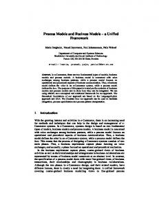
Figure 2: Demand curve and equivalent offer for an injection 3.1.4

Responsive load and load shedding specification

The generalized formulation employed in Matpower allows the specification of price-responsive loads as negative injections. For welfare maximization, the negative of the benefit function can be specified; market bids are assumed otherwise. Thus, a load demand as in Fig. 2 can be converted to a corresponding injection offer or “cost”. Because a load’s reactive consumption cannot be dispatched, price-responsive injections with negative active power are assumed to exhibit a constant power factor. This models the behavior of such loads more accurately and is a standard feature in Matpower. Load shedding can be modeled by specifying a demand curve whose first block’s price corresponds to that of the value of lost load. This approach is appropriate for maximization of social welfare, where the value of lost load should be taken into account. If the actual value of lost load should not be allowed to set the nodal prices at the solution, an alternative approach is to use whatever price caps are in effect in the market. This models load shedding in a setting in which the consumers are not compensated. It should be noted, however, that true load shedding is a non-convex problem; normally, if the first block in a load’s demand curve is made price-responsive to model load shedding, this does not mean that there is an ability to dispatch it half-

12

way through; in a normal OPF setting the solution algorithm might try to split the block. This would require an adjustment to the post-contingency flow in order to shed the whole block. 3.1.5

Reserve allocation in a day-ahead setting

Secure dispatch and post-contingency rescheduling requires that resources be available for redispatch if needed. Traditional security rules include the N − 1 spinning reserve criterion for each control area, in which the amount of reserve must be enough to cover the loss of the largest generation unit. Other rules specify 10 and 30 minute reserve as a percentage of the load being served. Non-integrated market approaches such as [18,19] require pre-specified amounts of reserve to be met, usually divided by zones. However, the true locational aspect of reserve has not always been addressed. The reserve resources must have an appropriate geographic distribution to be able to harness their energy should it be needed if a contingency occurs. Works such as [7–9] address exactly this issue, as opposed to, for example [21,22,28], in which an integrated market is optimized but the reserve amounts to be met are specified in a zone by zone basis, not a contingency analysis-originated basis. The direct formulation approach used there, without simplification of network constraints, is helpful for obtaining solutions that need no further adjustment. The approach suggested in [7] simply provides a solution from which it is feasible to transition to any of the postcontingency states considered; the raison d’ˆetre for reserve is implicit in the dispatch itself. In [8, 9], the concept of reserve amount and reserve contract is introduced, so that reserve markets can be designed, and a full AC flow setting is employed. This work expands [9] to consider both upward and downward excursions as “reserve”, albeit of a different kind, as well as reactive reserve. This makes it easier to integrate the approach to a day-ahead market-based scheduling framework in which there must be a real time follow-through. Other efforts have included [23–26] with a linear flow formulation. 3.1.6

Receding horizon, stochastic transition and cost framework

Security-constrained OPF models that rely on explicit formulation of post-contingency flows can be thought of as multi-scenario planning models with coupling constraints. These constraints are there to model transition-related limits, ramp rates in particular. This suggests a tree structure for the problem, the branches representing both transitions and coupling constraints. This approach has been suggested explicitly in the setting of unit commitment algorithms [11] but is certainly inherent in other “direct” treaments of the security-constrained OPF. In fact, this approach can 13

1,1

1,1,1

1,2

1,2,1

2,1

2,1,1

1

2 2,2

Figure 3: General tree structure for representation of transitions. be generalized further by allowing several tree structures in a single problem. This way, more than one probability-weighted “base case” can be considered, each with corresponding contingency-originated transitions and constraints, also probabilityweighted. The probability weightings used here can be computed from individual equipment failure rates and line outage probabilities based also on weather prediction, as well as historic data. The proposed scheme can be useful to model high-load and low-load predictions in addition to the central 24 hour-ahead load prediction. Of course, this adds to the dimension of the problem. An example of such a tree is shown in Fig. 3, which considers two base cases, with two contingencies considered for each. Here, an additional refinement has been introduced in that the transition to a post-contingency state can be modeled in two stages if necessary, the first being the immediate postcontingency state of the system, after voltage controls have acted, but before AGC has had a chance to correct frequency and area interchange; and a second and final stage in which economic redispatch is assumed to have taken place. In the proposed scheme, the cost of operation for every scenario is weighted by its probability of occurrence, making the problem one of constrained stochastic optimization. This makes economic sense as it solves for the least expected cost of

14

procurement. One could certainly consider (N − 2)-type contingencies sprouting from each of the terminal N − 1 contingency nodes, but it is clear that the dimensionality of the problem would become unmanageable with both current and envisioned computing capabilities. Even when the ramp limits are ignored and a linear (DC) network model is used as in [20], N − 2 security results in huge mathematical programs. This approach, in which the transition direction is important, is different from that considered in [8, 9], where the redispatch amount needed to transition between any two considered scenarios is bounded to be less than the available “ramp rate”. Thus the formulation in this work is less conservative. A related view of the problem is that of a receding-horizon optimal stochastic control problem. The N − 1 security translates to a one-stage horizon from the moment that the control actions are implemented, and the 24 hour-ahead planning translates to a 24-hour control delay. The probabilities employed in the formulation are those estimated day-ahead, which will certainly be different from those in real time, when there is little uncertainty about the load level and the weather. It is important to recognize this because the realized system state one day later is bound to be at least slightly different from the central day-ahead prediction, i.e. the base case. Thus, for completeness of the problem, any real-time or spot rescheduling mechanisms must be taken into account in the day-ahead planning. That is the reason why in this work additional costs on deviations from the contracted dayahead quantity are employed; these must be provided by participants in the market at the same time that they offer in the day-ahead energy and reserve market. 3.1.7

Base case dispatch vs. optimal procurement

A major feature of the proposed formulation is that the day-ahead contract quantities are not constrained to be equal to the base case dispatch. Rather, additional contracted quantity variables together with several sets of inequalities involving the incremental dispatches, reserve variables and actual base and post-contingency dispatches are employed. This offers more flexibility in selecting a day-ahead optimal contract to the independent system operator. In integrated, co-optimized markets this flexibility is actually needed in some cases to be able to reach an optimum hedge. When the contracted quantities are set to be equal to the base case dispatch, the shadow prices on energy may require modification and the system cost can increase.

3.2

Basic Nomenclature

15

pik , qik

ith active and reactive injection in kth post-contingency state (k = 0 for base case).

CP i (·), CQi (·)

Cost function for ith active and reactive injections.

pci , qci

Purchase amounts specified in the day ahead contract for active and reactive power from the ith injection.

+ p+ ik , qik

ith active and reactive upward deviations from contracted amount in k-th post-contingency state; k = 0 means realized deviation from contract with no contingencies.

+ CP+i (·), CQi (·)

Cost for incremental deviations from contract day-ahead quantity.

− p− ik , qik

ith active and reactive downward deviations from contracted amount in kth post-contingency state.

− CP−i (·), CQi (·)

Cost for decremental deviations from contracted day-ahead quantity.

+ rP+i , rQi

Upward active and reactive reserve amount provided by ith injection.

+ + CRP i (·), CRQi (·) Cost functions for upward reserve purchased from ith injection. − rP−i , rQi

Downward active and reactive reserve amount provided by ith injection.

− − CRP i (·), CRQi (·) Cost functions for downward reserve purchased from ith injection.

(Θk , V k , P k , Qk ) Voltage angles and magnitudes, active and reactive injections for power flow in kth post-contingency state (k = 0 means no contingency occured). g k (·)

Nonlinear power flow equations in kth post-contingency state.

hk (·)

Transmission, voltage, generation and other limits in kth postcontingency state.

πk

Probability of kth contingency (π0 is the probability of no contingency).

ng

Number of generators and dispatchable or curtailable loads initially available. 16

nc

Number of contingencies considered.

Gk

Set of indices of generators present in the kth contingency.

Individual variables can be grouped in vectors, such as pik into P k , and it will be consistent with the context.

3.3

Day-ahead problem formulation

For simplicity of notation, we consider a tree with only one root, namely, the base case. More subindices would be required for additional roots, perhaps replacing k by k j , with j being the root index. The functional to minimize is the expected cost min fP (P ) + fQ (Q) + fRP (RP ) + fRQ (RQ ) Θ, V, P, Q, P + , P − , Q+ , Q− , Pc , Qc , RP , RQ

(24)

where the active power cost component is fP (P ) =

nc X

πk

X h

i

− − CP i (pik ) + CP+i (p+ ik ) + CP i (pik ) ,

(25)

i∈Gk

k=0

with three sub-components. Here, πk is the probability of transition to the kth contingency from the day-ahead base case; CP i (pik ) is the production cost or offer for the ith generator in the kth contingency; CP+i (p+ ik ) is an incremental cost, additional to the production cost, on upward deviations from the quantity that is contracted for in the day ahead market. Similarly, CP−i (p− ik ) is an additional cost imposed on downward deviations from the day-ahead contract. These costs allow generators to signal a reluctance to vary their power output from the contracted day-ahead quantities, which can be valid for some types of base load units. Likewise, the reactive power cost is fQ (Q) =

nc X k=0

πk

X h

i

+ − + − (qik ) , CQi (qik ) + CQi (qik ) + CQi

(26)

i∈Gk

the active reserve cost is fRP (RP ) =

ng X

− − + + [CRP i (rP i ) + CRP i (rP i )],

i=1

17

(27)

and the reactive reserve cost is fRQ (RQ ) =

ng X

− − + + )]. (rQi ) + CRQi (rQi [CRQi

(28)

i=1

Here, upward and downward reserves define a dispatch range relative to the dayahead contracted quantities, (pci , qci ). Now, all of this is subject to nonlinear active and reactive power flow constraints in the base case flow and all contingencies, gPk (θk , V k , P k , Qk ) = 0,

k = 0 . . . nc ,

(29)

k gQ (θk , V k , P k , Qk ) = 0,

k = 0 . . . nc ,

(30)

transmission capacity, generation capability curve, voltage limit, dispatchable load power factor, and maximum angular separation constraints for all flows, hk (θk , V k , P k , Qk ) ≤ 0,

k = 0 . . . nc ,

(31)

and new, additional constraints that couple the base case and the post-contingency flows, defining the deviation variables and the reserve variables. The first three such constraints define upward deviations from contract quantity and upward reserves, + 0 ≤ p+ 0 ≤ qik , ∀i, k, ik ,

pik − pci ≤ p+ ik , + max+ p+ , ik ≤ rP i ≤ RP i

(32)

+ qik − qci ≤ qik , ∀i, k,

(33)

+ + max+ qik ≤ rQi ≤ RQi , ∀i, k.

(34)

The next three do the same for downward deviations and reserves, − 0 ≤ p− 0 ≤ qik , ∀i, k, ik ,

pci − pik ≤ p− ik , − max− p− , ik ≤ rP i ≤ RP i

(35)

− qci − qik ≤ qik , ∀i, k,

(36)

− − max− qik ≤ rQi ≤ RQi , ∀i, k.

(37)

Then, the deviations from the base case (not from the contracted amount) are bounded by the physical ramp rate of each unit, + −∆− P i ≤ pik − pi0 ≤ ∆P i − + −∆Qi ≤ qik − qi0 ≤ ∆Qi

∀i, k = 1 . . . nc .

(38)

Finally, these constraints allow imposing or relaxing an equality constraint between the contracted quantities and the base case dispatch quantities by choice of α −α ≤ pi0 − pci ≤ α −α ≤ qi0 − qci ≤ α 18

∀i,

(39)

so that the contracted quantity can be specified to be equal to the base case dispatch if so desired. In this formulation, for the bounds in (33,34,36,37) to be tight at the solution it is − + − + − + − necessary that marginal costs on deviations and reserves (p+ ik , pik , rP i , rP i , qik , qik , rQi , rQi ) be positive. They can be allowed to be zero but that may require adjusting the bounds to be tight as a post-solution procedure that does not affect the cost. Negative marginal costs are not acceptable for this formulation. − + − It is important to note that while the new (p+ ik , pik , qik , qik ) variables and con+ − straints still follow the structure of the actual modeled transitions, the (rP+i , rP−i , rQi , rQi ) variables and constraints bound all deviations from contracted quantities equally, and thus those constraints do not follow the structure exhibited by the transition tree. The solution to the day-ahead problem yields optimal day-ahead contract quanti+ − ties (Pc , RP+ , RP− , Qc , RQ , RQ ) as well as generation ranges; for all considered scenarios, the ith generator’s active output will lie in [pci − rP−i , pci + rP+i ], except perhaps in the scenario in which that unit is off line as a result of a contingency. The treatment of the reactive output is similar. It is thus that the results of the day-ahead planning materialize in a contract for providing a nominal quantity pci at a price that depends on the chosen auction institution and the marginal cost of energy at the generator’s location, with the additional obligation to abide by any redispatch issued by the ISO in real time within the range [pci − rP−i , pci + rP+i ], with such redispatch incurring the incremental costs, additional to those of energy alone, in the amount of the deviation from contract times the accorded price. This range of generation is reflected in the amounts of reserve rP+i and rP−i procured from the ith generator. A day-ahead settlement can be executed or the parties can wait until the real-time pricing and redispatch is performed the next day.

3.4

Real-time adjustment of dispatch

The problem of balancing and pricing the real-time market is now subject to the contract issued the previous day. Reserve quantities have already been determined and payed for; a generation range, together with the original energy and incremental energy offers and the current state of the network are what is available to the ISO to compute any needed redispatch. Incremental amounts and costs are now determined from the pci agreed upon the previous day. Security is still desirable, of course, and the dispatch should still consider the possibility of transitioning to other network configurations as a result of contingencies. At this point in time, however, the probabilities of occurence for contingencies have changed and in some cases, such as the specific realized demand, the uncertainty may no longer exist. The time viewpoint 19

available to the planner now is not the same as the one available the previous day. There is more information. Either the system is “intact” and exhibits the configuration of the base case (with perhaps a somewhat different demand) or a contingency has happened and the system has undergone a transition. 3.4.1

Redispatching the intact system

Assume that an intact system configuration is realized; that is, the configuration contemplated in the base case, possibly with a slightly different demand. While the transition restrictions needed to enforce a secure dispatch should still be included in the model, the probabilities of contingencies used for a pricing run of the model should be set to zero, i.e., the contingencies did not materialize. However, the formulation to follow could also be used for an hour-ahead or 10 minute-ahead redispatch, in which case some probabilities would not be zero. Thus, the problem at this stage becomes     C (p ) + C (q ) n P i ik Qi ik c   X X + + + + +CP i (pik ) + CQi (qik ) min (40) πk   − − − −  Θ, V, P, Q, k=0 i∈Gk  +CP i (pik ) + CQi (qik ) P +, P −, Q+ , Q− subject to gPk (θk , V k , P k , Qk ) = 0,

k = 0 . . . nc ,

(41)

k gQ (θk , V k , P k , Qk ) = 0,

k = 0 . . . nc ,

(42)

hk (θk , V k , P k , Qk ) ≤ 0,

k = 0 . . . nc ,

(43)

+ 0 ≤ p+ 0 ≤ qik , ∀i, k, ik ,

pik − pˆci ≤ p+ ik ,

+ qik − qˆci ≤ qik , ∀i, k,

(44) (45)

+ + p+ ˆP+i qik ≤ rˆQi ∀i, k, ik ≤ r

(46)

− 0 ≤ p− 0 ≤ qik , ∀i, k, ik ,

(47)

− pˆci − pik ≤ p− qˆci − qik ≤ qik , ∀i, k, ik ,

(48)

p− ˆP−i , ik ≤ r

− − qik ≤ rˆQi , ∀i, k,

+ −∆− P i ≤ pik − pi0 ≤ ∆P i − + −∆Qi ≤ qik − qi0 ≤ ∆Qi

∀i, k = 1 . . . nc ,

(49) (50)

+ ˆ− ˆ P+ , R ˆ P− , Q ˆ c, R ˆQ where (Pˆc , R , RQ ) are now parameters, taken from the day-ahead solution. There is no need to enforce box (Pmin , Pmax , Qmin , Qmax ) limits, since they are

20

+ − implicit in (ˆ rP+i , rˆP−i , rˆQi , rˆQi ). However, it should be noted that in generators with trapezoidal (pi , qi ) feasible regions like those employed in Matpower, the upper and lower sloped linear constraints should still be enforced (which Matpower does) and if binding, the corresponding multipliers can be decomposed into equivalent µPmax and µPmin multipliers to be taken into account.

3.4.2

Redispatching in a post-contingency state

Once the base case no longer describes the system configuration, possible transitions represent what would have been an (N − 2)-type event the day ahead. While the transition to the present state should have been feasible thanks to the resources committed day-ahead, it is by no means clear that transitioning to yet another state is allowed at this point. Yet, it makes sense to try to run the problem (40-50), with the base case replaced by the present system state and a set of (currently) credible contingencies, to see if it is still possible to redispatch the system securely and economically with the available resources.

3.5

Implementation

With the capabilities of the extensible OPF architecture described in section 2, it is possible to pose both the day-ahead and the real-time problems by first making copies of the original base case, modifying them to account for the equipment changes that give rise to each of the considered contingencies, and them lump all of these systems together in a big network with (nc +1) islands. The coupling constraints and the additional variables and linear constraints can be cast using the general linear constraint capability, while the costs on reserves and deviations from contract can be specified using the generalized cost component. This has been implemented in R Matlab for a single-root scenario tree which on all other accounts of the formulation is general and can be applied to any system in the Matpower data format. A single routine takes the original network data, performs the modifications on it according to a contingency modification data table, assembles the big disjoint system and specifies the additional linear constraints and generalized cost, proceeding then to call the generalized OPF solver in Matpower. This solver can in turn call R either Matlab ’s fmincon solver, or MEX-file solvers based on MINOS [33] and BPMPD [34] or those developed in [31].

21

3.6 3.6.1

Numerical considerations Solution tightness

Indeed, the day-ahead solution determined by the algorithm procures the reserve amounts needed in light of the scenarios considered and nothing more than that. Thus, if the scenarios do not capture the actual breadth of looming dispatch possibilities, it is possible that in real time, the procured reserve will prove to be inadequate. For the single-root scenario tree, it is therefore important to include not just equipment failures in the contingency set, but also deviations from forecasted load. Given an estimate of the uncertainty of the load forecast, it is possible to bound the estimate with 95 or 99% confidence interval brackets and use these as the lower and higher-than-expected demand scenarios. These two scenarios can capture locational demand differences if the uncertainty in the predictions is known down to a more local (bus or zone) level. 3.6.2

Completion of optimization in post-contingency dispatches

When the probabilities employed in some contingencies are very small, the contribution to the cost function by the injections considered in that contingency can be minimal. Therefore, it is possible that the optimizer being employed will stop the process after asserting that the corresponding portion of the gradient of the cost has a norm smaller than some tolerance, leading to an incomplete optimization of the dispatch for that contingency. This is a scaling issue inherent in the typical sets of probabilities employed in this problem; it would not be present if all outcomes were more or less equiprobable. It makes sense to run the real-time algorithm for each of the scenarios considered immediately after solving the day-ahead problem to see if there are any major differences in the dispatches obtained as a check on this issue. Note that a decomposition and coordination approach to solving this problem could potentially eliminate this scaling issue. 3.6.3

Larger scale implementation

For larger scale implementation, several issues still need to be addressed, among them the robustness and warm start capability of the underlying generalized OPF solver, the specific decomposition and coordination scheme used to separate the problems into smaller units for parallelization purposes, and the integration of the formulation into a unit commitment setting. This last issue may be resolved by employing the basic ideas in [29, 30].

22

4 4.1

Case Studies Maintaining Reliability Standards

Federal legislators have formally recognized the importance of maintaining operating reliability in the Energy Policy Act of 2005 (EPACT05), and the major effect of this legislation is to give the Federal Energy Regulatory Commission (FERC) the overall authority to enforce reliability standards throughout the Eastern and Western InterConnections (see FERC [36]). The North-American Electric Reliability Corporation (NERC) has been appointed by FERC as the new Electric Reliability Organization (ERO), and NERC has been given the responsibility to specify explicit standards for reliability. Although it is still too early to know how well these arrangements will work, it is clear that the threat of paying penalties will be a tangible reason for state regulators to ensure that reliability standards are met. In an electric supply system, the performance of the transmission network and the level of reliability are shared by all users of the network. Reliability has the characteristics of a “public” good (all customers benefit from the level of reliability without “consuming” it). In contrast, real electrical energy is a “private” good because the real energy used by one customer is no longer available to other customers. Markets can work well for private goods but tend to undersupply public goods, like reliability (and over-supply public “bads” like pollution). The reason is that customers are generally unwilling to pay their fair share of a public good because it is possible to rely on others to provide it (i.e. they are “free riders”). Some form of regulatory intervention is needed to make a market for a public good or a public bad socially efficient. If a public good or a public bad has a simple quantitative measure that can be assigned to individual entities in a market, it is feasible to internalize the benefit or the cost in a modified market. For example, the emissions of sulfur and nitrogen oxides from a fossil fuel generator can be measured. Requiring every generator to purchase emission allowances for the quantities emitted makes pollution another production cost. Regulators determine a cap on the total number of allowances issued in a region, and this cap effectively limits the level of pollution. Independent (decentralized) decisions by individual generators in the market determine the pattern of emissions and the types of control mechanisms that are economically efficient. For example, the choice between purchasing low sulfur coal and installing a scrubber is left to market forces in a “cap-and-trade” market for emissions of sulfur dioxide. Unfortunately, when dealing with the reliability of an electric supply system, it is impractical to measure and assign reliability to individual entities on the network

23

in the same way that emissions can be assigned to individual generators. This is particularly true for transmission lines that are needed to maintain supply when equipment failures occur. The NERC uses the following two concepts to evaluate the reliability of the bulk electric supply system (see NERC [40]): 1. Adequacy – The ability of the electric system to supply the aggregate electrical demand and energy requirements of customers at all times, taking into account scheduled and reasonably expected unscheduled outages of system elements. 2. Operating Reliability – The ability of the electric system to withstand sudden disturbances such as electric short circuits or unanticipated failure of system elements. Prior to EPACT05, the NERC standard of one day in ten years for the Loss of Load Expectation (LOLE) was widely accepted by regulators as the appropriate standard for the reliability of the bulk transmission system (i.e., this does not include outages of the local distribution systems caused, for example, by falling tree limbs and ice storms). Nevertheless, it is still very difficult to allocate the responsibilities for maintaining a standard of this type to individual owners of generating and transmission facilities because of the interdependencies that exist among the components of a network. This fundamental problem has not stopped regulators from trying to do it. The basic approach used by state regulators in New England, New York and PJM is to assume that setting reserve margins for generating capacity (i.e., setting a standard for “generation adequacy”) is an effective proxy for meeting the NERC reliability standard. This new proxy for reliability can now be viewed as the sum of its parts, like emissions from generators, and the task of maintaining generation adequacy can be turned over to market forces once the regulators have set a reserve margin. In New York State, regulators have gone one step further and passed the responsibility for purchasing enough generating capacity to meet the adequacy standard on to Load Serving Entities (LSE). Regulators decide what the amount of installed capacity should be in a region and the responsibility for acquiring this amount is prorated among the LSEs. An LSE that fails to comply would be fined (see NYISO [41] and [42]). In contrast, the ISOs in New England and PJM take the responsibility of purchasing the capacity needed in advance, and the cost is eventually prorated to LSEs using the actual load served in real time. This procedure identifies potential shortfalls of capacity in advance much more effectively than the NYISO procedure. 24

Even if the capacity markets are successful in maintaining generation adequacy, there are still important economic issues that are obscured when generation adequacy is used as a proxy for reliability. Changing a public good like reliability into a private good like installed capacity is a convenient sleight-of-hand for the advocates of deregulation because it then appears to be feasible to use market forces to maintain reliability standards. Nevertheless, this is not strictly correct because there is an implicit assumption that the transmission network is already adequate before decisions about generation adequacy are considered. It would be much more valuable for planning purposes to have a method of analysis that calculates the netsocial benefits of generation and transmission assets in terms of both the delivery of real power to customers and the maintenance of reliability standards. This is particularly important for evaluating the role of renewables on a network because these sources are typically intermittent and require additional reserve capacity (or storage capacity) to maintain reliability. Before presenting the new analytical framework in the next section, some of the practical implications of adding an unreliable source of electricity are discussed. The established reliability standard proposed by NERC is to limit failures to less than 1 day in 10 years. Is this standard too stringent, and therefore, more expensive to enforce than it should be? The answer is almost certainly no. The reason is that the Value of Lost Load (VOLL) when an unscheduled outage occurs is very high, particularly for large urban centers. A survey report published by the Lawrence Berkeley National Laboratory (LBNL) in 2004 (LaCommare and Eto [37]) concludes that the total cost of interruptions in electricity supply is $80 billion/year for the nation (op. cit. p. xi-xii), and 72% of this total is borne by the commercial sector (plus 26% by the industrial sector and only 2% by the residential sector). The frequency of interruptions is found to be an important determinant of the cost because the cost of an interruption increases less than proportionally with the length of an interruption. The costs of relatively short interruptions of only a few minutes are substantial. The cost estimates in the LBNL report are developed from an earlier report prepared for the Office of Electric Transmission and Distribution in the U.S. Department of Energy (DOE, Lawton et al. [38]) that summarizes a number of different surveys of the outage costs for individual customers. For large commercial and industrial customers in different economic sectors, the average costs are reported for 1-hour outages in $/Peak kW (op.cit. Table 3-3, p.13). These average costs range from negligible for Construction to $168,000/MWh for Finance, Insurance and Real Estate, and the average cost for all sectors is $20,000/MWh. Although there is a lot of variability in the reported costs of an unscheduled outage, the overall conclusion is that 25

the VOLL is very high for urban centers. The current NERC reliability standard of 1 day in 10 years corresponds to a VOLL of $33,393/MWh (60 + 80,000/2.4, based on an operating cost of $60/MWh and an annual capital cost of $80,000/MW for a peaking unit). Although this value is above the average value, it is still at the low end of the range of VOLL in the DOE report because the distribution of values is skewed to the right. The key to deriving the economic value of maintaining a given reliability standard is to consider the benefits of avoiding unscheduled outages. In the empirical simulations discussed later in Section 4.3, a VOLL of $10,000/MWh is used. Consequently, reducing the probability of an unscheduled outage by 0.1%, for example, still saves $10/MWh. The analytical framework presented in the following section treats equipment failures (contingencies) explicitly. Some components of a network may only have a positive economic value when contingencies occur because they reduce the amount of Load-Not-Served (LNS). Other components, such as a new baseload unit, may reduce the cost of generation when the system is intact and have little affect on reliability. More generally, components will affect both operating costs for the intact system and reliability. For an intermittent source such as wind power, there is a fundamental tension between providing an inexpensive source of generation and making the existing network more vulnerable to outages. The solution to this predicament is to add new capabilities to the network that can compensate for the intermittent nature of wind power, such as load response and storage capacity. Evaluating the net-benefits of a portfolio of assets is the type of problem that can be evaluated using our new analytical framework.

4.2

The Analytical Framework

In a typical restructured market operated by an Independent System Operator (ISO), like the market in the New York Control Area, standards of Operating Reliability are met by requiring that minimum amounts of reserve capacity (spinning reserves) are available in different regions. These reserve requirements are the proxy measures of reliability discussed in the previous section. The generators submit price/quantity offers to sell energy and reserves into an auction, and the objective of the ISO is to determine the optimal patterns of generation and reserves by minimizing the total cost (the combined cost of energy and reserves) of meeting a forecasted pattern of load subject to network and system constraints and the specified amounts of reserves. The Last Accepted Offer is used to clear the market and set uniform market prices for energy and reserves. The market prices are adjusted for congestion and losses to determine the nodal prices for energy (i.e. Locational Based Marginal Prices 26

(LBMP)). In addition, the auction determines the regional prices for reserves in a similar way. Given the large number of nodes (over 400 in the New York Control Area) and the complexity of the network, it is computationally impractical to use a full AC representation of network flows to determine the OPF for a system of this size. As a result, a modified version of a DC OPF is used by the NYISO. For example, if the real flows on a transmission line are limited by a voltage constraint on a regular basis, the rated thermal capacity of the line is reduced in the dispatch to approximate this voltage constraint (an AC representation of network flows determines both real and reactive flows, but a DC representation determines only real flows). Hence, the lower thermal constraint on a transmission line is really another form of proxy limit that provides an additional distortion for determining the true shadow prices of transmission constraints. These distortions of the nodal prices are similar in effect to specifying minimum quantities of reserve capacity as proxies for reliability. The implications of using proxy variables in an OPF will be discussed in more detail elsewhere. For this case study, the empirical analysis is based on an AC OPF using co-optimization to represent equipment failures (contingencies) explicitly in the objective function. 4.2.1

Fixed Reserve Requirements

To illustrate the specific differences between using co-optimization in an OPF instead of using the traditional fixed reserve requirements, it is convenient to start with the structure of an AC OPF using fixed reserve requirements. The formulation follows the pattern described by equations (15)–(20). Additional user variables, costs, and constraints, represented generically in section 2 by z, fu , and A, l, u, respectively, are required to add the fixed reserve portion. Suppose the reserve requirements are defined as a set of fixed zonal MW quantities. Let U denote the set of indices of all generators providing reserves, Zk be the set of generators in zone k and Rk specify the MW reserve requirement for zone k. A new variable ri is introduced for each i ∈ U , to represent the reserves provided by generator i. This value must be positive and is limited above, based on ramp rate, by rimax . 0 ≤ ri ≤ rimax (51) If the marginal cost of reserves from unit i is ci , the user defined cost term from (21) is simply X fu (x, z) = ci ri . (52) i∈U

27

resulting in an overall objective criterion to minimize the combined cost of energy, pi , and reserves, ri , needed to meet the forecasted pattern of load. There are two additional sets of constraints needed. The first ensures that, for each generator, the total amount of energy plus reserves provided does not exceed the capacity of the unit. pig + ri ≤ pi,max , ∀i ∈ U (53) g The second requires that the sum of the reserves available within each zone k meets the mandated levels of reserve capacity needed in different regions to cover the unscheduled failure of equipment. X

ri ≥ Rk ,

∀k

(54)

i∈Zk

In practice, determining the specified levels of reserves needed to meet the established standard of Operating Reliability depends on prior analyses, but it is likely that the actual mandated levels of reserve capacity are relatively conservative (i.e. high) to reduce the likelihood of facing the unpleasant political consequences of a blackout. If Generator i with capacity p∗i , for example, is part of the optimal dispatch for the intact system, it could have an unexpected failure. In this case, Generator i would be eliminated and the OPF would be solved again using only the other generating units committed in the first optimal dispatch, after lowering the appropriate reserve requirements in (54) by p∗i . Hence, the actual dispatch and the prices paid could be substantially different from the optimal solution for the intact system if a contingency occurs. Furthermore, there is no guarantee that an optimal solution will actually be feasible in a given contingency. The feasibility of the dispatch is dependent on there being enough reserve capacity available in the right locations to cover the contingency, and in practice, the mandated levels of reserves are reset relatively infrequently as the characteristics of the system change over time. 4.2.2

Responsive Reserves Requirements (Co-optimization)

Chen et al. [9] have proposed an alternative way to determine the optimal dispatch and nodal prices in an energy-reserve market using “co-optimization” (CO-OPT). The new objective is to minimize the total expected cost (the combined production costs of energy and reserves) for a base case (intact system) and a specified set of credible contingencies (line-out, unit-lost, and high load) with their corresponding probabilities of occurring. Using CO-OPT, the optimal pattern of reserves is determined endogenously and it adjusts to changes in the physical and market conditions 28

of the network. The initial motivation for developing the CO-OPT framework was to make the markets for reserves in load pockets less vulnerable to the exploitation of market power by generators. For this reason, the CO-OPT criterion is referred to as Responsive Reserve Requirements. If the offered prices for reserve capacity are high, the optimal solution will use fewer reserves by, for example, reducing the flow on a transmission tie line to reduce the size of the contingency if the tie line fails. This framework is equivalent to using a conventional n − 1 contingency criterion to maintain Operating Reliability. In practice, the number of contingencies that affect the optimal dispatch is much smaller than the total number of contingencies. In other words, by covering a relatively small subset of critical contingencies, all of the remaining contingencies in the set can be covered without shedding load. In the new SuperOPF formulation described in section 3, the reserve definition is modified to separate positive and negative reserves, now defined as maximum deviations from an optimal contracted dispatch. This new definition of reserve is essentially an agreement to re-dispatch within a specified range upon request. In addition, using the model for load shedding from section 3.1.4, with the price of each load j set to the value of lost load, V OLLj , the objective takes the form of maximizine expected social welfare. This is equivalent to minimizing overall expected cost with an explicit term for the cost of Load-Not-Served (LNS). cost of LNS =

nc X k=0

πk

 X 

j∈Lk

V OLLj × LN Sjk

 

(55)



where πk is the probability of contingency k occurring, V OLLj is the value of lost load for load j and LN Sjk is the amount of load j that is not served in contingency k. Since the reserves are defined by (34) and (37) as the maximum re-dispatch amounts needed to meet the explicit set of contingencies, rather than by the fixed requirements of (54), they are location-specific and are determined endogenously. The optimum quantities of energy and reserves are contracted ahead of real time and then the generators are also paid for the additional energy generated in real time. The maximum (minimum) dispatched capacity of every generator, Gmax and i min Gi , is needed for energy in at least one contingency. The level of reserve capacity for any generator is determined endogenously, and it responds to conditions on the network, such as the pattern of forecasted load. This feature is important for the case study on renewables due to the wide range of wind conditions that affect the actual generation from a wind farm and the difficulty in forecasting wind conditions accurately. The regulated standard of Operating Reliability is maintained if load is met in all of the contingencies. Finding optimal values of LN Sjk > 0 is equivalent to violating 29

this reliability standard, and it signals a failure of System Adequacy in a planning application that would be corrected by increasing the system capacity in some way. Since the VOLL is specified to be very large compared to typical market prices, it is important to note that a major part of the total benefit of many components of the grid comes from avoiding unscheduled load shedding when contingencies occur. When the system is Adequate, no failures of Operating Reliability will be observed, and therefore, it is no longer possible to use the observed market prices to determine the full net-benefit of an investment that was made to avoid unscheduled outages. These are the “Events that didnt Happen” that should be considered when calculating the economic value of reliability in a planning model (see Mount et al. [39]). One of the many useful capabilities of the SuperOPF is that the optimization can be considered in two stages. The first stage is the full co-optimization described in section 3.3 and it can be viewed as the optimum way to minimize the expected costs and maintain Operating Reliability when the system is Adequate (i.e. all LN Sjk = 0 for all credible contingencies). This stage determines the amounts and prices of energy and reserves contracted in advance of real time (e.g. one day ahead). The second stage corresponds to a real-time OPF when the actual state of the system is known and a contingency may have occurred. The objective cost is now to minimize the incremental cost of adjusting from the contracted amounts of resources from the first step to meet the actual system conditions. The second stage of the SuperOPF, described in section 3.4, treats the actual state as the new base (k = 0) and, assuming the system is still intact, includes all of the remaining contingencies. This implies that the optimum dispatch in the second stage still attempts to maintain Operating Reliability. However, if a major failure has already occurred, it may not be possible to meet the load in all situations if a second failure occurs. This would not be a violation of the typical standard of Operating Reliability assuming that the specification of the first stage covered all credible contingencies. For example, if the regulators define System Adequacy as the ability to cover all single failures, there is no guarantee that the system can cover the relatively rare event that two or more failures occur. Following any major contingency, bringing the system back into compliance with Operating Reliability would require adding existing resources that were rejected from the auction in the first stage of the optimization. The current practices adopted in restructured markets are more in line with the optimization for Fixed Reserve Requirements in (51)–(54), and the expected cost of meeting the contingencies is not explicitly part of the objective function. In the New York Control Area, for example, a modified DC OPF minimizes the expected cost of meeting load for the intact system with specified levels of reserves included. 30

If a contingency occurs, there is an ordered list of options, such as using reserve capacity and exercising contracts for interruptible load, with shedding load as the least desirable option. Since the contingencies are not considered explicitly in the optimization, it is virtually impossible to determine the true economic benefit of reliability from the market solutions, and meeting a given reliability standard is treated as a physical constraint rather than as an explicit economic component of the objective function as it is in the SuperOPF. After a contingency occurs, the objective in the SuperOPF is still to minimize the expected cost over all contingencies even if this requires shedding some load in some contingencies. The amount and location of load shedding is determined optimally. For example, if the VOLL in an urban region is much higher than the VOLL in other regions, the solution will implicitly put more weight on avoiding the shedding of load in the urban area. In fact, the SuperOPF is consistent with the relatively successful market design in Australia. In the Australian system, the market clears in real time every five minutes to meet load and to set the prices paid for the energy generated over the following five-minute period. These are the only prices used by the system operator to pay for energy. There are also forward markets, but these markets are financial and are not run or regulated by the system operator. The five-minute auction for energy includes a market for regulation and fast-responding reserves. These ancillary services receive payments for the reserve capacity contracted at the beginning of each five-minute period and for any energy that is actually generated. This is just like the first stage of the SuperOPF, but in the Australian market, the second stage never occurs. The five-minute auctions are like a continuous series of first stage optimizations. Capacity rejected in one period can still be entered into the next periods auction. Consequently, when a contingency occurs, the next market solution will bring new capacity into the market that was not needed (i.e. rejected from the auction) before the contingency occurred. The incentive for ensuring that additional capacity will be ready to enter the market is provided to generators and loads by reporting forecasts of the prices a few hours ahead. These forecasted prices are determined by the existing offers and bids that have been submitted in advance but they are not binding for making payments. All payments for energy and ancillary services are made using the real-time prices. When the forecasted prices are high, and the price cap of $10,000A/MWh is relatively high in the Australian market, more generators are likely to enter the market and loads may adopt procedures for reducing demand in anticipation of the high prices. Another important feature of the Australian market is that the responses to a contingency before the next five-minute market clears are preset and automatic by, 31

for example, using smart appliances as a fast way to shed load for a short period of time in response to a drop in frequency. The following section describes the characteristics of the network used for the case study and the specifications of the simulations. The basic objective of the analysis is to evaluate the effects of increasing the load in a load pocket on Operating Reliability when the amount of installed generation and transmission capacity is fixed. The initial amounts of installed capacity are sufficient to meet the standard for System Adequacy and meet the load in all of the credible contingencies. As the load increases, standards of System Adequacy can no longer be maintained and some load has to be shed in some of the contingencies. In this case study, the focus is on showing how the analytical structure of the SuperOPF makes it possible to identify at what level of load and where on the network problems first occur. An important implication for regulators is that the high cost of shedding load is often localized in the sense that the high market prices are limited to a few nodes. As a result, the best way to fix a problem may be to add Distributed Energy Resources (DER) close to the affected loads rather than increase the capacity of the bulk power transmission network.

4.3

The Specifications for the Case Study

The case study is based on a 30-bus network that has been used extensively in our research to test the performance of different market designs using the PowerWeb platform. The one-line-diagram of this network is shown in Figure 4 below. The 30 nodes and the 39 lines are numbered in Figure 4 and this numbering scheme provides the key to identifying the locations of specific contingencies, constraints and shadow prices in the following discussion. In addition, the six generators are also identified. The network is divided into three regions, Areas 1–3, and Area 1 represents an urban load center with a large load, a high VOLL and expensive sources of local generation from Generators 1 and 2. The other two regions are rural with relatively small loads, low VOLLs and relatively inexpensive sources of generation from Generators 3–6. Consequently, an economically efficient dispatch uses the inexpensive generation in Areas 2 and 3 to cover the local loads and as much of the loads in Area 1 as possible. The capacities of the transmission tie lines linking Areas 2 and 3 with Area 1 (Lines 12, 14, 15 and 36) are the limiting factors. Since lines and generators may fail in contingencies, the generators in Area 1 are primarily needed to provide reserve capacity. The general structure of the network poses the same type of problem faced by the system operators and planners in the New York Control Area. Most of the load is in New York City (i.e. Area 1) and the inexpensive sources of baseload capacity (hydro, coal and nuclear) are located upstate (i.e. Areas 2 and 3). 32

Figure 4: The One-Line-Diagram of the 30-Bus Network.

33

In this case study, the simulation increases the load in Area 1 in small increments until the capacity of the network is no longer able meet all loads in all contingencies. In other words, the standards for Operating Reliability and System Adequacy are eventually violated after the load has been increased sufficiently. The amounts and locations of the different types of installed generating capacity are shown in Table 1 together with the production costs. The levels of load and generation by Area are shown for the initial conditions (i.e. the lowest aggregate load) in Table 2. The total amounts of generating capacity in each Area are similar in Table 1, but the corresponding costs of production vary a lot and are much higher in Area 1. Table 1: Installed Generating Capacity and Production Costs by Type and Location Nuclear Combined Gas Total Area Coal Oil Hydro Cycle Gas Turbine by Area 1 – – 65 MW – 45 MW 110 MW 2 50 MW 70 MW – – – 120 MW 3 65 MW – – 40 MW – 105 MW Total by 115 MW 70 MW 65 MW 40 MW 45 MW 335 MW Type Production $5 $25 $95 $55 $80 – Cost ($/MWh) Table 2 shows that the initial system load is less than half the capacity of installed generating units, and under these conditions, the network has a lot of excess generating capacity. There is no generation in Area 1 in the base case (intact system) and transfers from Areas 2 and 3 are used to meet the load. However, 17 MW are needed in Area 1 (33% of Load) to cover the contingencies (Gen. (max) – Gen. (base)). Exactly the opposite situation exists in Areas 2 and 3, and the levels of generation are substantially higher than the corresponding loads. The additional capacity needed to cover contingencies is smaller than the levels of generation in the base case, and the amounts of idle capacity (i.e. not used in any contingency) are relatively small in Areas 2 and 3 (21 MW) compared to Area 1 (93 MW). More of this unused capacity will be used as the load increases in Area 1, and the simulation covers a wide range of network conditions that illustrate clearly how the different types of constraint on network capacity affect nodal prices. By maintaining Operating Reliability using the initial set of conditions on the network, there is an implicit assumption that the system is robust enough to meet all loads in all credible contingencies. The specific contingencies included in this case study are listed in Table 3. These contingencies include the failures of individual 34

Table 2: Initial Patterns of Load and Generation by Area Gen. % of Gen. % of Gen. % of Area Load Idle (base) Load (min) Load (max) Load MW MW MW MW MW 1 50.7 0.0 0% 0.0 0% 16.8 33% 93.2 2 56.2 91.8 163% 73.6 131% 115.8 206% 4.2 3 48.5 65.0 134% 59.3 122% 87.1 180% 17.9 Total 155.4 156.8 101% 132.9 86% 219.7 141% 115.3 Gen. (base) Generation for the intact system Gen. (min) Lowest generation in a contingency Gen. (max) Highest generation in a contingency Inst. Installed capacity

% of Load 184% 8% 37% 74%

Inst. MW 110.0 120.0 105.0 335.0

generators and transmission lines, and also the uncertainty about the actual level of load caused by the errors of forecasts when the optimum dispatch is determined a day ahead of real time, for example. For generators and lines, there are only two possible outcomes. The first outcome is to perform as required in the optimum dispatch, and the second is to fail completely. However, the probability of failure is very small (0.2% for each failure in this case study), and as a result, the probability that each piece of equipment will perform as required is 99.8%. Since there are 15 failures identified in Table 3, the expected number of failures is 3 in 100 periods because the individual failures and periods are specified to be statistically independent. In other words, the system is expected to be intact 97% of the time. The last two contingencies correspond to errors in load forecasting, and there is a 1% probability that the system load will be substantially higher (lower) than the forecasted level. This capability to deal with uncertainty about load in the SuperOPF is even more useful when variable sources of generation such as wind turbines are part of the network. The basic structure of the simulation is to increase the five loads in Area 1 by proportional increments holding the pattern of loads constant in Areas 2 and 3. For each step in the simulation, the SuperOPF determines the optimal dispatch to meet load and maintain Operating Reliability using the 17 contingencies listed in Table 3. The expectation is that initially, as load increases in Area 1, generation in Areas 2 and 3 will increase until transmission limits on the tie lines are reached. When this happens, further increases in load will be covered by increases in generation from the expensive sources in Area 1. The market will fragment and the prices in the load pocket (Area 1) will be substantially higher than the prices in the Areas 2 and 3. 35

% of Load 217% 214% 217% 216%

k 0 1 2 3 4 5 6 7 8 9 10 11 12 13 14 15 16 17

Table 3: The Contingencies Used in the Case Study Contingency Probability = base case 95.0% = line 1 : 1–2 (between gens 1 and 2, within area 1) 0.2% = line 2 : 1–3 (from gen 1, within area 1) 0.2% = line 3 : 2–4 (from gen 2, within area 1) 0.2% = line 5 : 2–5 (from gen 2, within area 1) 0.2% = line 6 : 2–6 (from gen 2, within area 1) 0.2% = line 36 : 27–28 (main tie, areas 1–3) 0.2% = line 15 : 4–12 (main tie, areas 1–2) 0.2% = line 12 : 6–10 (other tie, areas 1–3) 0.2% = line 14 : 9–10 (other tie, areas 1–3) 0.2% = gen 1 0.2% = gen 2 0.2% = gen 3 0.2% = gen 4 0.2% = gen 5 0.2% = gen 6 0.2% = 10% increase in load 1.0% = 10% decrease in load 1.0%

36

Eventually, the capacity of the network will be insufficient to meet all loads in all contingencies, implying that the standard of Operating Reliability has been violated. This failure to meet all loads will occur first in one or more of the contingencies when equipment fails. Finally, the load will be so high that some load must be shed in the Base Case to obtain a feasible solution for the optimum dispatch. When this happens, the expected price is effectively at the VOLL at all nodes shed load. In practice, it is difficult to predict exactly where on the network the high prices associated with load shedding will occur. Load shedding in a contingency may, for example, be caused by a voltage constraint on a specific transmission line. By incorporating the AC constraints on line flows in the optimization, this is exactly what the SuperOPF does well. The distortions caused by using proxy limits for network capacity in standard planning models tend to be more severe in these extreme situations when the network is stressed. By identifying the specific locations of the high prices where loads are shed, important information is provided for planning purposes to help determine exactly where on the network reliability has failed and what needs to be fixed. This is a necessary first step in determining whether the investment cost of upgrading the network to avoid load shedding can be justified in terms of the economic benefits from not shedding load. In simple terms, if the amount of load shed and the probability of this happening are both very small, the expected benefit may be smaller than the certain cost of financing the investment, and the investment would not be economically efficient. Even the most reliable network will fail to cover some very rare contingencies, such as cascading failures of equipment. The important point is that the structure of the SuperOPF makes it possible to evaluate the economic implications of meeting reliability standards instead of treating reliability as a set of additional physical constraints on network operations using, for example, minimum amounts of reserve generating capacity in different locations. There are two different sources of uncertainty that need to be identified before evaluating the economic benefit of an investment in upgrading the capacity of a network. The first source comes from the inherent uncertainty about the state of the system in a co-optimization because the objective function in (24) determines the expected outcome over a set of different contingencies. It is not certain in a dayahead market, for example, exactly what the state of the network will be in real time. The optimal dispatch determined by the SuperOPF represents a contracted pattern of generation and of upwards and downwards reserves, and the corresponding nodal prices (shadow prices) are the expected prices over the set of contingencies listed in Table 3. Maintaining Operating Reliability corresponds to having no unscheduled outages in any of the contingencies, and this is the case for the initial conditions summarized in Table 2. The main physical restriction on the choice of an optimal 37

dispatch is that it must be possible to meet any one of the contingencies starting from the intact system (k = 0) without violating ramping constraints. The second source of uncertainty is associated with the variability of the levels of load during a year. The expected economic value of an investment should consider the expectation over different contingencies and over different levels of load. The decrease in the expected annual cost of operating the system after making an investment in increased network capacity is the correct economic measure to compare with the annualized cost of financing this investment. In a planning application, the incremental increases in the loads in Area 1 discussed at the beginning of this section can be treated as the increases in the forecasted annual peak load for the system. Implicitly, it is assumed that if no load shedding is observed in any of the contingencies for a given peak load then Operating Reliability can be maintained for the other, lower levels of load throughout the year. In other words, the scheduling of the maintenance of generating units during the year is organized in a sensible way to avoid unscheduled outages, and for this case study, all generators are assumed to be available throughout the year to keep the analysis simple. As soon as standards of Operating Reliability for a specified peak load are violated (because load shedding occurs in some contingencies), the network capacity is no longer Adequate and this is a signal that additional economic analysis is warranted to investigate whether violations also occur at lower levels of load. For this case study, the different levels of load that occur during a year are specified to be consistent with the patterns of loads in New York City and Long Island (for Area 1) and in upstate New York (for Areas 2 and 3) for a year with a relatively hot summer (2005). All loads within Area 1 and within Areas 2 and 3 vary proportionally to the aggregate loads in each of the regions. The simulation breaks a year into 100 equal steps and the corresponding scaled LDCs for each region are shown in Figure 5. Since both the LDC start at 100%, the relatively low values of the LDC for Area 1 imply that the loads in Area 1 are more affected by air conditioning in the summer than the loads are in Areas 2 and 3. These procedures are used to complete the link between the annualized cost of an investment and the expected annual benefit from lower operating costs, and this link is essential for determining the net benefit of an investment. However, the procedures for specifying the pattern of loads during a year represent a rough approximation, and the loads used correspond to a single realization of the actual hourly time-series of loads in two regions. Incorporating the range of possible realizations of hourly load that could occur during a year will be the focus of future research.

38

SCALED LOAD DURATION CURVES 120

Percentage of the Peak Load

100

80

60

40

20 Area 1 Area 2 & 3

0 0

10

20

30

40

50

60

70

80

90

100

Percentage of the Year

Figure 5: The Scaled Load Duration Curves for Area 1 and for Areas 2 and 3

39

4.4

Results of the Simulation

The simulation for this case study has two components. The first component starts with the network shown in Figure 4 and the initial conditions for installed capacity and costs summarized in Tables 1 and 2. The loads in Area 1 are then increased in proportional increments until the specified standard of Operating Reliability is violated. These loads represent the peak loads on the network as levels of demand increase over time. The second component of the simulation takes a specific level of peak load when the network is no longer “Adequate” and is unable to meet all loads in all contingencies. The simulation then determines the expected production costs for the annual pattern of loads described in Figure 5. This second component of the simulation makes it possible to determine the expected cost of violating the reliability standards.

Figure 6: Expected Nodal Prices for Generators as the Peak Load Increases The prices shown in Figure 6 represent the expected nodal prices for the six generators as the peak load on the network is increased (The “Scale Factor” measures the scale of the load in Area 1). Each nodal price is derived from the shadow prices determined by the SuperOPF in equation (29), and it is the expectation of the 40

shadow price over the list of contingencies shown in Table 3. Actual real-time prices would be different because more precise information about the state of network would be incorporated into determining these prices. For example, if a major piece of equipment has failed, the real-time prices in some locations may be much higher than they would have been if the system had remained intact. However, these high prices are weighted by a small probability when the expected nodal prices in Figure 6 are computed, and the biggest weight is put on the prices for the Base Case when the system is intact (Contingency 0 in Table 3). At low levels of load (Scale Factor < 0.9), the nodal prices in Figure 6 are low and the price differences among the generators are small. Note that the nodal prices for Generators 1 and 2 can still be computed even though these units are only needed for reserve capacity when the system is intact. Under the low-load conditions, the network has a lot of excess transmission capacity and all loads can be met with generation from the baseload units. The coal units set the market prices at $25/MWh, and the small differences in the nodal prices reflect losses because there is no congestion on the network. When the system load increases sufficiently (Scale Factor > 0.9), congestion on the network occurs and the nodal prices for Generators 1 and 2 increase substantially to almost $70/MWh and finally to $90/MWh because the expensive units in Area 1 are needed to meet the load. The lowest prices in Figure 6 are for Generator 3 in Area 3 because the tie line from Area 3 to Area 1 (L36) and the adjoining distribution lines within Area 1 have limited capacity, and as a result, this unit is isolated by the network and cannot benefit from the high prices at other locations. Generators 5 and 6 in Area 2 do benefit from the higher prices even though the main tie line from Area 2 to Area 1 (L15) does get congested at high levels of load. The expected nodal prices for the loads in the three areas are shown in Figure 7. Even though the behavior of these prices for most loads follows a similar pattern to the prices for the generators in Figure 6, the price for the load at Bus 8 is an anomaly and it increases to almost $10,000/MWh for the highest levels of load (Scale Factor > 1.30). This high price is the VOLL in Area 1 and it implies that some load at Bus 8 is being shed when the system is intact. In fact, all prices above $90/MWh for this bus are due to load shedding. When load shedding is limited to rare contingencies, the effect on the expected price is small and the expected price increases as load is shed in more of the contingencies. Eventually, load is shed in all contingencies including the Base Case when no equipment failures occur. There are two important implications for system planning that can be drawn from the prices in Figure 7. First, the results derived by the SuperOPF show when and where potential violations in reliability standards occur (i.e. load shedding at 41

Figure 7: Expected Nodal Prices for Loads as the Peak Load Increases

42

Bus 8), and as a result, they raise the important question, what is so special about the load at Bus 8? Why is the network able to meet the other loads in Area 1 and not meet the load at Bus 8? Second, the high prices at Bus 8 are very localized and have surprisingly little effect on the other nodal prices in Area 1. This suggests that the best solution for upgrading the network to meet reliability standards may be to add Distributed Energy Resources close to Bus 8 rather than to upgrade the tie lines into Area 1, for example. A simple way to interpret the price changes in Figures 6 and 7 is to treat the initial increased differences in prices at different nodes as an indication of congestion on the tie lines into Area 1. The existence of a persistently large price difference between a low price region (Areas 2 and 3) and a high price region (Area 1) is the conventional rationale for upgrading transmission capacity on a tie line that is used by economists and advocates for merchant transmission projects. There is nothing basically wrong with this argument. The net benefits of a transmission upgrade should be evaluated if there are substantial amounts of inexpensive generation that could be built but could not be delivered to loads over the existing network. In fact, this was the main justification used by the FERC for encouraging merchant transfers and open access to the bulk power transmission network in Order 888. In fact, the type of analysis used to address network congestion is very similar to the typical economic analysis used to justify upgrading the capacity of a pipeline for natural gas. There is a potential problem if economic analyses are limited to “pipeline” thinking when evaluating a transmission upgrade on an electric delivery system because it ignores the economic value of reliability. The large increase of the nodal price at Bus 8 in Figure 7 when the Scale Factor > 1.3 reflects the cost of having an unreliable network. It is quite possible in practice that the expected costs of these unscheduled outages are much larger than the expected costs of congestion because the VOLL in financial centers like New York City is so high. The overall conclusion is that a sound planning process should be able to evaluate the net economic benefits of both removing congestion and maintaining reliability standards, and in reality, it may be very difficult to allocate the cost of a specific upgrade in capacity to the “economic” component and the “reliability” component in a scientific way. A major benefit of using the SuperOPF is that both components are evaluated simultaneously as part of the standard optimization. The expected costs of unscheduled load shedding are shown in Figure 8 for the different contingencies identified in Table 3. When the Scale Factor (referred to as the Load Factor in Figure 8) increases from 1.05 to 1.25, load shedding occurs in three different contingencies and the expected costs of load shedding are above zero, 43

but when the Scale Factor is above 1.3, load shedding occurs in most contingencies. These high levels of load correspond to the jumps in the nodal prices in Area 1 seen in Figures 6 and 7. When the Scale Factor is above 1.35, load shedding occurs in the Base Case (Contingency 0), and as a result, the expected cost is close to the VOLL (note that the price scale in Figure 8 is logarithmic). As the system load increases in Figure 8, the following sequence of situations can be identified: 1) no load shedding occurs at low loads, 2) load shedding is localized to a small number of contingencies at slightly higher loads, 3) increasing the load further causes load shedding for almost all of the contingencies representing equipment failures, and finally 4) load is shed in the Base Case at the highest loads.

Expected Load Shedding Cost 18

4.5

16

4

Contingency

14

12

3.5

10

3

8

2.5

6

2

4

1.5

2

1

0

0.5

0.6

0.7

0.8

0.9

1

1.1

1.2

1.3

1.4

1.5

1.6

Scale Factor for Load

Figure 8: Expected Costs of Unscheduled Load Shedding in Different Contingencies The discussion turns now to identifying what goes wrong when the load in Area 1 44

is increased sufficiently to cause load shedding at Bus 8, and which component(s) of the network should be fixed to maintain Operating Reliability and avoid shedding load at these higher levels of load. It should be noted, however, that the standard output from the SuperOPF computes shadow prices for all potential real and reactive constraints on the network for each one of the contingencies specified in Table 3. Hence the results that follow represent a highly selective sample that were chosen after screening all of the computed shadow prices to locate constraints that were binding (i.e. have non-zero shadow prices). In addition, there are many different ways to present these results. For example, the expected nodal prices in Figures 6 and 7 are the weighted averages of the shadow prices for real energy taken over all contingencies at the specific nodes for generators and loads, respectively. In contrast, the expected prices in Figure 8 are the weighted averages of the shadow prices for specific contingencies taken over the nodes for loads weighted by the amount of load shed. Furthermore, the underlying shadow prices for each node/contingency combination are determined before the actual network conditions are known using the probabilities of different contingencies occurring shown in Table 3. These shadow prices may not be exactly the same as the corresponding real-time shadow prices after a specific contingency has actually occurred and new information has been incorporated into the optimization. The shadow prices determined by the SuperOPF represent predictions for different contingencies based on the best information available at the time. Figures 9 and 10 illustrate the shadow prices for specific transmission constraints that are caused by congestion and by load shedding, respectively. The shadow prices for different contingencies on the tie line from Area 2 to Area 1 (Line 15 in Figure 4) are shown in Figure 9 (note that Contingency 7 is the failure of Line 15, and therefore, the corresponding shadow prices cannot be computed). The non-zero shadow prices are caused by congestion that becomes apparent in some contingencies at relatively low levels of load (Scale Factor > 0.65), and congestion occurs for the Base Case (Contingency 0) when the Scale Factor is above 0.85. Nevertheless, the highest shadow price shown in Figure 9 is still relatively low (< $100/MWH) even when the system load is at its highest level. Figure 10 shows the shadow prices for Line 10 in the different contingencies. These prices reach $10,000/MWh in some contingencies when the Scale Factor is above 1.1, and in the Base Case (Contingency 0) when the Scale Factor is above 1.3. These levels of load correspond exactly to the levels of load in Figure 8 when load shedding occurs at Bus 8. It should be noted that Line 10 is not a major tie line into Area 1 but only a distribution line within Area 1 that links Bus 8 to Bus 6. The limited capacity of this line at higher levels of load is responsible for 45

Flow Limit Shadow Price @ Branch 15 : 4−12

Contingency

18

16

80

14

70

12

60

10

50

8

40

6

30

4

20

2

10

0 0.6

0.7

0.8

0.9

1

1.1

1.2

1.3

1.4

1.5

1.6

Scale Factor for Load

Figure 9: Shadow Prices for Line 15 Caused by Congestion

46

Flow Limit Shadow Price @ Branch 10 : 6−8 18

10000

16

9000

14

8000

7000

Contingency

12

6000 10 5000 8 4000 6 3000 4 2000 2 1000 0 0.6

0.7

0.8

0.9

1

1.1

1.2

1.3

1.4

1.5

1.6

Scale Factor for Load

Figure 10: Shadow Prices for Line 10 Caused by Load Shedding

47

the load shedding at Bus 8 that violates the standard of Operating Reliability. An important implication for planning is that it is generally much easier to predict where congestion problems are likely to occur on a network than it is to predict the location of reliability problems. Using knowledge of the levels of generation and costs of installed generating units, congestion occurs if some inexpensive units are not fully dispatched for energy or reserves. In practice, large differences in the nodal prices at different locations on the network indicate where this congestion is likey to be. On the other hand, reliability problems may be highly localized and hard to identify because they are associated with rare contingencies and may never actually be observed in a market. In fact, if standards of System Adequacy are maintained on a network, the high shadow prices associated with load shedding should not be observed. Furthermore, system operators often suspend market operations after major contingencies have occured so that the resulting high shadow prices are ignored. For these reasons, it is much better to deal with reliability issues before problems occur using appropriate analytical tools as part of an established planning process than it is to fix problems following an actual blackout. In the long run, maintaining reliabilty standards on an electric delivery system is just like maintaining other forms of infrastructure like bridges. It is very expensive and potentially dangerous to wait until things break before fixing them. The final step in the analysis is to determine the expected annual cost of meeting load using the patterns of load shown in Figure 5. In this case study, the optimal dispatch for different levels of load that occur during a year can be computed in exactly the same way as they are for the different levels of load in Figures 6–10. Since the levels of load in Figures 6–10 represent the peak loads on the network, binding constraints are less likely to occur during the year at the lower levels of load, and as a result, the economic costs of congestion and load shedding will be smaller. At the lowest levels of load, the optimal dispatch will tend to be close to a merit order dispatch and the differences in nodal prices will be small, just as they are in Figures 6 and 7 at low levels of load. Figure 11 shows how the averge shadow price charged to loads can be split into different components of cost for the ranked system loads in different hours in the year. The horizontal axis “Percentage of the Year” is consistent with the ranked loads in Figure 8. The underlying system load decreases moving from left to right. A peak system load of 200MW (Scale Factor = 1.1278) is chosen for the initial network conditions so that load shedding occurs in some contingencies (see Figure 8). Each plot line in Figure 11 is calculated as the expected revenue/cost over all contingencies summed over all relevant nodes (e.g. the nodes for each generator for the production 48

cost) and divided by the total system load before any load shedding occurs. In this way, all of the variables in Figure 11 are measured in $/MWh and are calibrated in terms of the average price/cost per MWh demanded by customers with no outages.

Expected Total Costs/Prices per MW of Nominal Load 70 Energy Cost Energy Price Energy+Reserve Price Load Price Load+LNS Price

60

Cost/Price, $/MWh

50

40

30

20

10

0

10

20

30

40

50

60

70

80

90

100

Percentage of the Year

Figure 11: Components of the Average Price Paid by Loads During a Year The two highest lines in Figure 11 represent the demand side of the market. The average price paid by loads (Load Price) corresponds to the expected nodal prices computed by the SuperOPF. The highest line (Load + LNS Price) includes the cost to customers of Load-Not-Served (LNS) (i.e. LNS x VOLL). In practice, the amount paid to the system operator by loads does not include the VOLL for customers who were served at a node where the load of some other customers was shed involuntarily. Furthermore, the customers at that node who actually faced outages are not compensated. 49

For the supply side of the market, the lowest line in Figure 11 represents the average production cost of meeting the system load (Energy Cost). Since generators are paid the shadow price at the appropriate node, the price actually paid for energy (Energy Price) is usually higher than the true production cost. Figure 11 also shows the average of payments for energy and reserves (Energy + Reserve Price). In this example, the cost of purchasing reserves is relatively small. It should be noted that the reported payments to generators include only the payments for real power and real reserves. However, the SuperOPF does actually compute the corresponding payments for reactive power and reactive reserves, but in this example, these payments are trivially small. In contrast, the nodal prices for loads include the cost of buying reactive power implicitly because each load is specified to have a fixed load factor. Figure 12 shows the equivalent breakdown as Figure 11 in terms of the total hourly payments for different levels of system load during the year. The difference between the Energy Revenue and the Energy Cost measures the net revenue paid to generators above production costs that can be used to cover capital costs. This net revenue is large if expensive peaking units set a high price for baseload units with low production costs, and this is the situation when the Percentage of the Year is less than 70%. For lower levels of load with Percentage of the Year above 70%, the baseload units set the price and the net revenue is essentially zero. For low levels of system load (high values of Percentage of Load), customers pay prices that are very similar to the prices paid to generators. This implies that there is little congestion on the network. In contrast, loads pay a lot more than generators receive at higher levels of load, and this difference can be attributed to increasing congestion on the transmission network. For the highest levels of system load (Percentage of the Year < 10%), the true cost of generation increases and the payments to generators and by loads increases substantially more. This is when congestion on the network becomes severe, and finally when some load is shed, there is a spike in the average payments made by loads. Aggregating the costs, revenues and payments in Figure 12 over all hours of the year provides the basic information needed to evaluate the effects of congestion and reliability on the aggregate market outcomes and the implications for the participants on the demand side and the supply side. Although the results presented are aggregated, this type of information can also be computed for individual nodes, and therefore, the implications for a load or a generator at any particular location can also be determined. In addition, by evaluating the nodal price differences and flows on a specific transmission line, the same type of information can be determined for transmission owners. The aggregate annual values of the different components presented in Figure 12 50

Expected Total Cost/Revenue 14000

12000

Cost/Revenue, $

10000

8000

Energy Cost Energy Revenue Energy+Reserve Revenue Load Revenue Load+LNS Revenue

6000

4000

2000

0

10

20

30

40

50

60

70

80

90

100

Percentage of the Year

Figure 12: Components of the Hourly Payments Made by Loads During a Year

51

Table 4: Expected Annual Payments, Revenues DEMAND SIDE 1 Load Payment + Cost of LNS* 2 Load Payment SUPPLY SIDE 3 Energy + Reserves Revenue 4 Energy Revenue 5 Energy Cost DERIVED VALUES 6 Reliability Cost of LNS* (1 - 2) 7 Congestion Cost (2 - 3) 8 Net Revenue for Generators (4 - 5) * LNS is Load-Not-Served

and Costs ($/Year) $26,062,479 $26,058,061 $24,792,467 $24,506,897 $9,020,838 $4,418 $1,265,594 $15,486,059

are shown in Table 4 for the whole network. In addition, the corresponding costs of unreliability (shedding load), congestion and the net revenue above production costs for generators are computed. In this example, the expected cost of shedding load is very small (< $5,000/Year), and as a result, it is probably too small to justify fixing the problem. Using a conventional economic criterion, if the annualized cost of an investment to upgrade Line 10 is less than this amount, it would be economically beneficial to make the investment. Even though the VOLL is $10,000/MWh when load is shed, the amount of load shed is very small and the probability of the contingencies actually occurring in which load is shed is also very small. When these two features are combined, the implied amount of expected load shed is less than 0.5MW/Year for the system as a whole ($4,418 divided by the VOLL of $10,000). The NERC standard of limiting unscheduled outages to less than one day in ten years (< 2.4 Hours/Year) does not specify the quantity affected. However, it is probably realistic to interpret the NERC rule as stating that no load node should experience a complete outage for more than 2.4 hours in a year. In contrast, the SuperOPF allows partial outages to occur in which the loads for some customers at a node are shed but not for all customers at that node. Reconciling the economic and NERC definitions of reliability for a bulk power transmission system will be the subject for future research using the SuperOPF. For this particular example, the cost of congestion in Table 4 (> $1.2million/Year) is nearly 300 times larger than the cost of failing to maintain reliability. However, making an investment to reduce congestion requires the evaluation of a number of

52

different candidate transmission lines for upgrading the network. This is exactly the type of analysis that can be done using the SuperOPF. In our experience, persistent high price differences on a transmission line are a necessary but not a sufficient condition for getting an economic return from upgrading the capacity of that line on a meshed network. However, the line with the phantom price differences are generally located next to the line that is really causing the congestion. This is another topic for future research. The final derived cost in Table 4 is the net revenue above operating costs paid to generators. This cost (> $15million/Year) is over ten times greater than the cost to the system of congestion. In this example, most of the “excess” money paid by customers above the true operating costs goes to pay generators, and there is no mandate in a deregulated market about how this money should be spent. Even though this example is only a special case, the results raise the question of who is really benefiting from deregulation, and from the point of view of reliability, do the excess payments made by loads above out-of-pocket expenses provide the correct economic incentives needed to maintain standards of Operating Reliability? A casual answer to the question is no, and once again, this topic will be the focus of future research. The costs presented in Table 4 illustrate, in aggregate, the types of information that can be derived from the SuperOPF. In terms of evaluating any proposed upgrade to an existing network, the capabilities of the SuperOPF could be used to calculate how the individual components of the annual costs of running this network change with and without a specified investment. This is exactly the type of capability that regulators should have available when evaluating the net public benefit of proposed changes to a networks capabilities. In practice, the conventional analytical procedures used by regulators fall far short of having this essential analytical capability. A basic criterion for judging planning models in the future should be that they can evaluate the economic consequences of congestion and reliability simultaneously for any AC network specification.

4.5

Conclusions

The main purpose of this section is to illustrate how the new SuperOPF developed by PSERC researchers at Cornell can be used to determine the net social benefit of system reliability on a network with a specified pattern of loads. The important features of the SuperOPF are 1) failures of equipment (contingencies) are considered explicitly in the optimization, 2) load shedding at a high Value-of-Lost-Load (VOLL) is allowed in all contingencies, and 3) the optimization incorporates the 53

nonlinear constraints of a full AC network. These three features make it possible to 1) determine the correct shadow prices for different components of the network under different operating conditions, 2) calculate the correct net social benefit of maintaining Operating Reliability, and 3) evaluate the net economic benefit of an investment that lowers expected production costs. In contrast, most conventional algorithms for determining the dispatch of generators simplify the nonlinear computations by using proxy limits on network capacity, such as lowering the thermal limits of transmission lines. These proxy limits inevitably distort the shadow prices computed in the optimization. Furthermore, proxy measures, such as minimum reserve margins for generating capacity in different locations, are included in the optimization as additional constraints to represent the Operating Reliability. This procedure makes Operating Reliability a physical constraint rather than an economic requirement. In reality, the economic benefits of some components of a network are determined exclusively by avoiding the high cost of unscheduled outages when equipment fails in relatively rare contingencies. In the SuperOPF, the shadow prices and the level of Operating Reliability reflect the actual operating conditions, and high shadow prices tend to occur under adverse conditions when the network is congested due, for example, to high levels of load or equipment failures. These adverse situations are the most important for determining the true economic benefit of different components of a network, but these situations are exactly the ones in which the shadow prices are the most distorted using conventional algorithms. Using conventional dispatching algorithms, it is potentially misleading to use the observed nodal prices of real power and ancillary services in a market as a guide for identifying what should be fixed on a network when standards of Operating Reliability are violated. The fundamental limitations of conventional planning tools are largely responsible for the attempt by many regulators to make a clear distinction between “economic” investments and “reliability” investments when planning capacity expansions. Although this is a convenient simplification, this practice completely ignores the true economic benefit of maintaining a high level of reliability. In reality, most upgrades of a network, particularly of transmission lines, affect both production costs and reliability. Determining how much of the capital cost of a specific upgrade should be treated as a reliability upgrade versus an economic upgrade is quite arbitrary using conventional planning tools. Reliability should be treated as an economic decision that depends on the actual operating characteristics of the network. Using the SuperOPF, shedding load at specific locations in one or more contingencies is an explicit indication that the level of reliability has deteriorated and where on the network the problems have occurred. 54

The basic planning decision is to determine whether an investment in upgrading capacity is justified by showing that the annual cost of this investment is less than the product of the high value of the Load-Not-Served times the small probability that the contingencies in which the outages happen actually occurs. Basically, it is not economically efficient or practical to avoid outages in all possible contingencies. The case study presented in this paper demonstrates how the SuperOPF can be used to address reliability questions using an analytical framework that links the short-run criterion of Operating Reliability with the long-run criterion of System Adequacy in a consistent way.

References [1] O. Alsac and B. Stott, “Optimal load flow with steady state security,” IEEE Trans. Power App. Syst., vol. PAS-93, no. 3, pp. 745–751, May 1974. [2] R.C. Burchett and H.H. Happ, “Large scale security dispatching: An exact model,” IEEE Trans. Power App. Syst., vol. PAS-102, no. 9, pp. 2995-2999, Sept. 1983. [3] B. Stott and E. Hobson, “Power System Security Control Calculations Using Linear Programming, Parts I and II,” IEEE Trans. Power App. Syst., vol. PAS97, no. 5, pp. 1713-1731, Sept. 1978. [4] B. Stott and J.L. Marinho, “Linear programming for power system network security applications,” IEEE Trans. Power App. Syst., vol. PAS-98, no. 3, pp. 837– 848, May 1979. [5] A. Monticelli, M.V.F. Pereira, and S. Granville, “Security-constrained optimal power flow with post contingency corrective rescheduling,” IEEE Trans. Power Syst., vol. 2, no. 1, pp. 175–181, Feb. 1987. [6] B. Stott, O. Alsac, and A.J. Monticelli, “Security analysis and optimization,” Proc. IEEE, vol 75, no 12, pp. 1623–1644, Dec. 1987. [7] J.S. Thorp, C.E. Murillo-S´anchez, and R.J. Thomas, “Time-space methods for determining locational reserves: A framework for location-based pricing and scheduling for reserve markets,” Cornell University, Nov. 2001. [8] J. Chen, J.S. Thorp, R.J. Thomas, and T.D. Mount, “Locational pricing and scheduling for an integrated energy-reserve market,” in Proc. 36th Annual Hawaii International Conf. on System Sciences, Jan. 2003. 55

[9] J. Chen, T.D. Mount, J.S. Thorp, and R.J. Thomas, “Location-based scheduling and pricing for energy and reserve: a responsive reserve market proposal,” Decision Support Systems, vol. 40, no. 3, pp. 563–577, Oct. 2005. [10] J.M. L´opez-Lezama, C.E. Murillo-S´anchez, L.J. Zuluaga, and J.F. Guti´errezG´omez, “A contingency-based security-constrained optimal power flow model for revealing the marginal cost of a blackout risk-equalizing policy in the colombian electricity market,” in Proc. 2006 Transmission and Distribution Conference and Exposition: Latin America. [11] P. Carpentier, G. Cohen, J.-C. Culioli, and A. Renaud, “Stochastic optimization of unit commitment: a new decomposition framework,” IEEE Trans. Power Syst., vol. 11, no. 2, pp. 1067–1073, May 1996. [12] J. Carpentier, D. Menniti, A. Pinnarelli, N. Scordino, and N. Sorrentino, “An algorithm for direct solution of active secure economic dispatch with an improved economic statement,” in Proc. Powercon 2000, vol. 3, pp. 1239–1244. [13] J. Carpentier, D. Menniti, A. Pinnarelli, N. Scordino, and N. Sorrentino, “A model of the ISO insecurity costs management in a deregulated market scenario,” in Proc. 2001 IEEE Porto Power Tech Conf. [14] P. Damrongkulkamjorn and T.W. Gedra, “Optimal power flow with expected security costs,” presented at 31st Annual Frontiers of Powers Conf., Stillwater, Oklahoma, Oct. 26–27, 1998. [15] J. Condren, T.W. Gedra, and P. Damrongkulkamjorn, “Optimal power flow with expected security costs,” IEEE Trans. Power Syst., vol. 21, no. 2, pp. 541–547, May 2006. [16] F. Capitanescu and L. Wehenkel, “Improving the statement of the corrective security-constrained optimal power-flow problem,” IEEE Trans. Power Syst., vol. 22, no. 2, pp. 867–889, May 2007. [17] Y. Fu, M. Shahidehpour, and Z. Li, “AC contingency dispatch based on securityconstrained unit commitment,” IEEE Trans. Power Syst., vol 21, no. 2, pp. 897– 908, May 2006. [18] R.J. Kaye, F.F. Wu. and P. Varaiya, “Pricing for system security,” IEEE Trans. Power Syst., vol 10, no. 2, pp. 575–583, May 1995.

56

[19] H. Singh and A. Papalexopoulos, “Competitive procurement of ancillary services by an independent system operator”, IEEE Trans. Power Syst., vol. 14, no. 2, pp. 498–504, May 1999. [20] R.A. Jabr, A.H. Coonick, and B.J. Cory, “A homogeneous linear programming algorithm for the security constrained economic dispatch problem”, IEEE Trans. Power Syst., vol. 15, no. 3, pp. 930–936, Aug. 2000. [21] M. Madrigal and V.H. Quintana, “A security-constrained energy and spinning reserve market clearing system using an interior-point method,” IEEE Trans. Power Syst., vol. 15, no. 4, pp. 1410–1416, Nov. 2000. [22] T. Wu, M. Rothleder, Z. Alaywan, and A.D. Papalexopoulos, “Pricing energy and ancillary services in integrated market systems by an optimal power flow”, IEEE Trans. Power Syst., vol. 19, no. 1, pp. 339–347, Feb. 2004. [23] F. Bouffard, F.D. Galiana, and A.J. Conejo, “Market-clearing with stochastic security—Part I: Formulation,” IEEE Trans. Power Syst., vol. 20, no. 4, pp. 1818–1826, Nov. 2005. [24] J.M. Arroyo and F.D. Galiana, “Energy and reserve pricing in security and network-constrained electricity markets,” IEEE Trans. Power Syst., vol 20, no. 2, pp. 634–643, May 2005. [25] F.D. Galiana, F. Bouffard, J.M. Arroyo, and J.F. Restrepo, “Scheduling and pricing of coupled energy and primary, secondary, and tertiary reserves,” Proc. IEEE, vol 93, no 11, pp. 1970–1983, Nov. 2005. [26] S. Wong and J.D. Fuller, “Pricing energy and reserves using stochastic optimization in an alternative electricity market,” IEEE Trans. Power Syst., vol 22, no. 2, pp. 631–638, May 2007. [27] F. Milano, C.A. Ca˜ nizares, and A.J. Conejo, “Sensitivity-based securityconstrained OPF market clearing model,” IEEE Trans. Power Syst., vol 20, no. 4, pp. 2051–2060, Nov. 2005. [28] O.E. Moya, “A spinning reserve, load shedding, and economic dispatch solution by Bender’s decomposition,” IEEE Trans. Power Syst., vol. 20, no. 1, pp. 384– 388, Feb. 2005.

57

[29] C.E. Murillo-S´anchez and R.J. Thomas, “Thermal unit commitment including optimal AC power flow constraints,” in Proc. 31st. Annual Hawaii International Conf. on System Sciences, [30] C.E. Murillo-S´anchez and R.J. Thomas, “Thermal unit commitment with a nonlinear AC power flow network model,” in The next generation of electric power unit commitment models, B.F. Hobbs, M.H. Rothkopff, R.P. O’Neill, and H.P. Chao, Eds., Kluwer Academic, 2001, pp. 75–92. [31] H. Wang, C.E. Murillo-S´anchez, R.D. Zimmerman, and R.J. Thomas, “On computational issues of market-based optimal power flow”, IEEE Trans. Power Syst., vol. 22, no. 3, pp. 1185–1193, Aug. 2007. [32] R.D. Zimmerman, C.E. Murillo-S´anchez, Matpower User’s Manual, Version 3.2, [Online]. Available: http://www.pserc.cornell.edu/matpower/. [33] B.A. Murtagh and M.A. Saunders, MINOS 5.5 User’s Guide, Stanford University Systems Optimization Laboratory technical report SOL 83-20R. [34] C. M´esz´aros, “The efficient implementation of interior point methods for linear programming and their application”, Ph.D. thesis, E¨otv¨os Lor´and University of Sciences, 1996. [35] C.W. Taylor, Power system voltage stability, McGraw-Hill, 1994. [36] Federal Energy Regulatory Commission (FERC), Energy Policy Act of 2005 (EPACT05), Washington DC, 2005. [37] K. H. LaCommare and J. H. Eto, Understanding the cost of power interruptions to U.S. electricity consumers, Ernest Orlando Lawrence Berkeley National Laboratory, Berkeley, CA (US), 2004. [38] Lawton, Leora, Michael Sullivan, Kent Van Liere, and Aaron Katz (Population Research Systems, LLC) and Joseph Eto (LBNL), A Framework and Review of Customer Outage Costs: Integration and Analysis of Electric Utility Outage Cost Surveys, Office of Electric Transmission and Distribution, U.S. Department of Energy, Washington DC, November 2003. [39] Mount, Tim, Alberto Lamadrid, Surin Maneevitjit, Bob Thomas and Ray Zimmerman, The Economics of Reliability and the Importance of Events that Didnt Happen, Invited Presentation at the Fourth Annual Carnegie-Mellon University Conference on the Electricity Industry, March 2008. 58

[40] North-American Electric Reliability Corporation (NERC), 2007 Long-Term Reliability Assessment 2007-2016, Princeton NJ, October 2007. [41] New York Independent System Operator (NYISO), 2004 Load and Capacity Data, Rensselaer NY, 2004. [42] New York Independent System Operator (NYISO), Comprehensive Reliability Planning Process Draft Reliability Needs Assessment, Rensselaer NY, September 2005.

59