Superposition method for calculating singular stress fields at kinks ...

International Journal of Fracture 102: 99–139, 2000. © 2000 Kluwer Academic Publishers. Printed in the Netherlands.

Superposition method for calculating singular stress fields at kinks, branches and tips in multiple crack arrays J. KENNETH BURTON JR.1∗ and S. LEIGH PHOENIX2 1 Department of Physics, Cornell University Ithaca, NY 14853, U.S.A. 2 Department of Theoretical and Applied Mechanics, Cornell University, Ithaca, NY 14853, U.S.A.

Received 10 September 1998; accepted in revised form 6 January 1999 Abstract. A method is developed for calculating stresses and displacements around arrays of kinked and branched cracks having straight segments in a linearly elastic solid loaded in plane stress or plain strain. The key idea is to decompose the cracks into straight material cuts we call ‘cracklets’, and to model the overall opening displacements of the cracks using a weighted superposition of special basis functions, describing cracklet opening displacement profiles. These basis functions are specifically tailored to induce the proper singular stresses and local deformation in wedges at crack kinks and branches, an aspect that has been neglected in the literature. The basis functions are expressed in terms of dislocation density distributions that are treatable analytically in the Cauchy singular integrals, yielding classical functions for their induced stress fields; that is, no numerical integration is involved. After superposition, nonphysical singularities cancel out leaving net tractions along the crack faces that are very smooth, yet retaining the appropriate singular stresses in the material at crack tips, kinks and branches. The weighting coefficients are calculated from a least squares fit of the net tractions to those prescribed from the applied loading, allowing accuracy assessment in terms of the root-mean-square error. Convergence is very rapid in the number of basis terms used. The method yields the full stress and displacement fields expressed as weighted sums of the basis fields. Stress intensity factors for the crack tips and generalized stress intensity factors for the wedges at kinks and branches are easily retrieved from the weighting coefficients. As examples we treat cracks with one and two kinks and a star-shaped crack with equal arms. The method can be extended to problems of finite domain such as polygon-shaped plates with prescribed tractions around the boundary. Key words: Stress intensity factors, interacting kinked cracks, wedges.

1. Introduction When modeling fracture evolution in elastic materials, calculating the stress and displacement fields for an arbitrary array of strongly interacting cracks is very difficult. As such cracks grow, some may kink or branch or join others forming a variety of crack sizes and geometries, as shown in Figure 1. To map this evolution realistically, one needs not only the stress intensity factors (SIFs) for crack tips, but also the exponents and intensities of singular stresses at kinks or branches, where new tips may initiate. Furthermore, knowing the full stress field will be essential for treating nucleation of new cracks. In the literature, various techniques have been used to approach such problems but with limited success. Complex variable methods have yielded closed form, analytical solutions, but only for a few simple configurations or periodic arrays. Perturbation methods have been used on kinked cracks (e.g. Cotterell and Rice, 1980), but inaccuracies arise at large kink angles. Conformal mapping techniques may be used on branched cracks (e.g. Chatterjee, 1975) but numerical difficulties are often encountered. More ∗ Present address: Dell Computer Corporation, One Dell Way, Round Rock, TX 78682, U.S.A.

100 J. Kenneth Burton Jr. and S. Leigh Phoenix

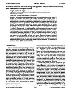
Figure 1. Original multi-crack problem decomposed into a trivial problem (no cracks and nonzero far-field stress) and an auxiliary problem (nonzero crack-face tractions and zero far field stress).

general configurations have required numerical or hybrid numerical-analytical approaches such as superposition based on influence functions, the distributed dislocation technique, the finite element method or the boundary element method. These methods have generally neglected singular stresses at crack kinks and branches. Also, computational requirements become prohibitive for large arrays. 1.1. S UMMARY

OF PAST APPROACHES

One approach we call the traction-based influence function method superimposes stress fields for certain single crack problems. In these ‘unit’ problems, the key task is to tailor the crack face tractions, sometimes called ‘pseudotractions’, such that after superposition the resulting stress fields yield the correct net tractions for the overall problem. In particular, the important problem of a crack with an array of microcracks near its tip has received much attention. Various versions of the method have been given by Hoagland and Embury (1980), Chudnovsky and Kachanov (1983), Chudnovsky et al. (1987a, 1987b), Hori and NematNasser (1987), Gong and Horii (1989), Kachanov et al. (1990), Laures and Kachanov (1991), and Meguid et al. (1991). Other problems, such as T-shaped and H-shaped cracks were treated

Superposition method for calculating singular stress fields 101 by Benveniste et al. (1989), and Dvorak et al. (1992). Additional examples are given in Datsyshin and Savruk (1973), Gross (1982), Chen (1984), Horii and Nemat-Nasser (1985), Yang and Liu (1993) and Atluri (1997). Most versions have used truncated, polynomial expansions of the crack-face tractions, where coefficients are found from a large system of linear algebraic equations. To treat very large arrays of straight interacting cracks, certain simplifications in the interactions were introduced by Kachanov et al. (1990), and Laures and Kachanov (1991). Kachanov (1994) gives an extensive review of the traction-based influence function method. A powerful approach known as the distributed dislocation technique developed in Bilby and Eshelby (1968), formulates crack interaction problems in terms of systems of singular integral equations with Cauchy kernels. Various applications have appeared in the literature, such as those by Lo (1978), Hayashi and Nemat-Nasser (1981), Zang and Gudmundson (1988), Hu and Chandra (1993), Chen and Hasebe (1995) and Han and Wang (1996). Common solution methods use versions of Gauss–Chebyshev quadrature as developed in Erdogan et al. (1973), or Lobatto–Chebyshev quadrature as developed in Theocaris and Ioakimidis (1977) where the usual goal is to obtain crack-tip SIFs. An approach by Gerasoulis (1982), however, uses piecewise quadratic polynomials along the crack line yielding integrals which can be evaluated exactly. A similar approach, used in mining research, models individual cracks as end-to-end sequences of short cuts with polynomial opening displacements (usually rectangular or triangular) so that the integrals can again be evaluated exactly. Crack tip openings, however, are not modeled as having the usual parabolic shape. Examples in two-dimension are given by Crouch (1976), Napier (1990), and Napier and Peirce (1997), and in three-dimension, by Linkov et al. (1998). We also mention hybrid versions of such problems involving dislocation distributions for kinks and branches attached to the ends of straight cracks. This approach has been used by He and Hutchinson (1989) and Niu and Wu (1997). A monograph by Hills et al. (1996) describes in detail and distributed dislocation technique. The boundary element method (BEM) is also used to solve crack problems as described for example in a monograph by Aliabadi and Rooke (1991), and in a recent review by Cruse (1996). Application of BEM is not straightforward since the standard methodology is mathematically degenerated along the crack line. Modifications have often involved using special discretization of crack line integrals in terms of distributed dislocations, as for example in Chang and Mear (1995). Multi-crack problems have also been tackled using an approach involving weighted superposition of certain edge potential functions, as in Dwyer and Pan (1995) and Dwyer and Amadei (1995). Potential functions used have been line edge and auxiliary polar functions, cavity and crack edge functions, and vertex functions capturing crack tip and wedge singularities. The finite element method, using singular tip elements, is popular in solving crack problems. Banks-Sills (1991) gives a review. In this method the whole body must be discretized using fine meshes near crack tips and wedges, so computational requirement are typically very large, and error analysis is problematic. Issues also remain on how to handle interpolation at crack tips, as pointed out by Gray and Paulino (1998). A simpler discretization approach is the spring network model, which Curtin and Scher (1990a, b) used to study interacting crack-like structures. In this model, certain artifacts in the fracture process may occur as shown by Jagota and Bennison (1995). Attempts to avoid meshing involve ‘element-free’ Galerkin methods as described in Fleming et al. (1996), but degree-of-freedom requirements appear to be similar.

102 J. Kenneth Burton Jr. and S. Leigh Phoenix 1.2. D IFFICULTIES

WITH PREVIOUS APPROXIMATE SOLUTION METHODS

In solving problems with many cracks, traction-based influence function methods are efficient so long as cracks are straight and reasonably separated. But in problems with closely spaced tips, as may occur with collinear cracks, the opening displacement profiles distort radically at the inner tips. In many versions, the single-crack tractions are expanded in terms of finite polynomials. The basic difficulty is that in the limit as the two cracks join, the single-crack, traction distribution is divergent at each crack tip. As Kachanov (1994) points out, even a very small ligament between cracks suppresses the SIFs at outer tips, so traction expansions at inner, singular-like points must be accurate. Thus the degrees of such polynomials must be increased radically as the tips become closer. Consequently, methods built on polynomial traction expansions are likely to be poorly suited to treating kinked or branched cracks viewed as adjoining straight cracks. In large, multi-crack arrays, the simplified method of Kachanov and colleagues (see Kachanov, 1994) determines the tractions for a crack as the sum of imposed tractions plus the induced tractions from other cracks acting as though each is isolated (with an elliptical opening) but with a certain weight based on interactions through special traction averaging. The SIFs for the two crack ends are obtained numerically by a standard integral involving the single crack tractions. The method works well provided the cracks are not too close, but errors cannot be reduced arbitrarily because there is no flexibility to adjust the degrees of freedom (DOF). In principle, the distributed dislocation technique can overcome the shortcomings just discussed. A major difficulty, however, is the proper treatment of singularities at crack kinks and branches. A common approach is to write the dislocation density components µ1 (s) and µ2 (s) (tangential and normal), in distance s from a kink or branch, as the product of two functions, µj (s) = β(s)φj (s); the function φj (s) is taken as bounded, often a polynomial, but following Williams (1952), the function β(s) is taken to have the singular form β(s) ∼ s λ−1 near s = 0 where 1/2 < λ < 1 is a real singularity exponent (ignoring 0 or 1) for the wedge at the kink with material angle 2π − ω > π . (For ω < ωc = 1.7848 radians (102.55 degrees) two λ values satisfy 1/2 < λ < 1; the smaller corresponds to symmetric (mode I) deformation, and the larger to antisymmetric (mode II) deformation. For ωc < ω < π , there is only one value corresponding to mode I.) A solution method, tried by He and Hutchinson (1989) on kinked cracks, was to choose φj (s) as a polynomial of degree n and take β(s) as above. This led to the need for very careful numerical integration in many of the singular integrals, requiring a large computational expenditure. Since they were mainly interested in SIFs at the crack tips, He and Hutchinson employed a second, simpler approach based on Gauss–Chebyshev quadrature and used earlier by Hayashi and Nemat–Nasser (1981). Specifically it was assumed that λ = 1/2 and φj (0) = 0 whereby the singular integrals could be evaluated exactly, thus reducing the computation time, but slowing the convergence in n. The assumptions λ = 1/2 and φj (0) = 0 were also used by Niu and Wu (1997), and λ = 1/2 was used in the recent monograph by Hills et al. (1996) (see pp. 90–92) in preference to a cumbersome Gauss–Jacobi quadrature technique mentioned in their Appendix B. The latter authors, however, allowed φj (0) 6 = 0, introducing two conditions on φ1,a (0), φ2,a (0), φ1,b (0) and φ2,b (0) (a pair each for crack segments a and b flanking the kink), which was said to preserve the angle of the kink. Zang and Gudmundson (1988) also worked with a version of the form for µj (s) above, introducing certain constraints connected with ensuring mode I wedge singular behavior, but in the end assumed λ = 1 in example calculations.

Superposition method for calculating singular stress fields 103 An argument often used for making such approximations on kink or branch singular behavior is that using the ‘correct’ λ values for the mating wedges yields little improvement in calculating the SIFs for the crack tips. As we see later, one should not expect much improvement if one does not allow all the natural freedoms of both singular distortion and relative displacement of the mating wedge surfaces. One must include translation and rotation of one wedge relative to its mate associated with λ = 0 and 1, respectively. Corresponding to each eigenvalue λ (including 0 and 1) there happen to be several natural freedoms and relationships between φ1,a (0) and φ2,a (0) on one side of a kink to φ1,b (0) and φ2,b (0) on the other. These aspects appear to have been neglected in previous work, resulting in the need for many additional degrees of freedom (i.e., higher degrees of polynomials for φj,i (s)) to compensate locally at kinks and branches. Of course, the opportunity to calculate generalized SIFs for the wedge singularities is lost. 1.3. O UTLINE

OF THE PAPER

In treating arrays of kinked and branched cracks, there are advantages to a formulation in terms of integral equations with unknown dislocation distributions or opening displacement profiles (ODPs), rather than influence functions based on certain crack-line traction profiles. In following the first approach, our key idea is to develop basis fields derived from certain basis ODPs (opening and tangential) over material cuts we call ‘cracklets’, both of which are motivated by the local crack geometry. These basis ODPs are chosen to be analytically treatable inducing stress and displacement fields given in terms of straightforward classical functions, thus avoiding any numerical integration. Certain basis ODPs induce fields that are specifically chosen to reflect the stress singularities associated with wedges at crack kinks or branches, and others provide additional shaping. In isolation, several of the ‘building block’ ODPs produce nonphysical stress and traction singularities, but after weighted superposition of relatively few, unwanted singularities cancel out. What remains are smooth net, crack-face tractions that are extremely close to those prescribed (often zero in the actual problem), as well as the appropriate singular stresses in the wedge material. In essence the method allows flexibility, efficiency and precision in shaping the crack opening displacements. An important and novel aspect is that in the superposition, certain natural constraints are derived and applied to automatically eliminate unwanted singular tractions at wedge tips, yet retaining the appropriate singular stress behavior in the material as well as freedom of wedge movement and distortion. Then calculating the weighting coefficients involves a least squares fit of the net tractions to those prescribed. Accuracy is assessed both through the root mean square error and through convergence of the SIFs. The method gives an accurate analytical representation of the full stress field, without numerical integration, as well as SIFs for the crack tips and generalized SIFs for the kink singularities. Section 2 introduces the idea of ‘cracklets’ and the fundamentals of the solution method, and Section 3 develops the basis functions for the cracklet ODPs. Section 4 develops the solution strategy and Section 5 gives the SIFs for the crack tips and kink singularities. Section 6 applies the method to certain test problems, demonstrating the need for certain basis terms. We consider (i) a V-shaped crack loaded in far field tension, (ii) a horizontal straight crack partitioned into two and three cracklets, respectively, to see the effects of subdividing long cracks into segments, (iii) a crack with two kinks of different angles, and

104 J. Kenneth Burton Jr. and S. Leigh Phoenix (iv) a star-shaped crack studied recently by Chen and Hasebe (1995). We compute mode I and II SIFs both for crack tips and kink singularities whose exponents we determine. Section 7 concludes with a discussion of possible improvements to the method to speed convergence at the kink singularities. Also mentioned are potential extensions to treating bounded regions with nonuniform applied tractions, small scale tip fracture processes, and crack face interference. Appendix A gives analytical details on evaluating certain integrals used in calculating stress and displacement fields, and Appendix B formulates the nonsingularity constraints for crack face tractions at kinks and branches. Examples of many closely interacting cracks in a finite or infinite plate are left to a sequel. 2. Decomposition of cracks into cracklets and fundamentals of solution method We consider an infinite, isotropic, linearly elastic solid in two-dimension that has several, arbitrarily placed cracks that may be kinked or branched, as shown in Figure 1. Our attention is restricted to cracks that have straight segments in between any kinks or branch points. We assume an x–y Cartesian coordinate system, and apply a far field stress, σ ∞ , uniform in x and y, with the crack faces kept traction-free. Our goal is to calculate the resulting stress, strain and displacement fields in the material. As is common, we decompose this ‘original’ problem into two sub-problems: The first is the ‘trivial problem’ of and infinite body without cracks and with applied far field stress σ ∞ , and the second is the ‘auxiliary problem’ of the original body under zero far field stress but with traction τ = (τx , τy ) = −σ ∞ · ζ applied along each crack face, where ζ = (ζx , ζy ) is the crack face normal that depends on the orientation of the particular crack face and position along it (see Figure 1). The solution to the original problem is the superposition of the solutions to these two problems. In the trivial problem, the stress field is uniformly σ ∞ , and the displacement fields are easy to determine. Thus, the main task is to solve the auxiliary problem. 2.1. D ISLOCATION

DISTRIBUTIONS ALONG CRACK LINES AND CONCEPT OF A CRACKLET

For convenience of presentation, we imagine a single, continuous curve C, which travels a meandering path through the body, passing along the crack lines and through the material from crack tip to crack tip. In effect, the cracks are viewed as segments along this curve, which must be self-intersecting if the cracks are branched. We parameterize this curve in x and y as C(t) = (Cx (t), Cy (t)), where t is distance along it. The opening displacements of the cracks along C are the relative displacements of their upper and lower surfaces, and these are represented in terms of a dislocation distribution pair, (µ1 , µ2 ) = (µ1 (t), µ2 (t)), which are the derivatives with respect to t of the opening displacements in the x and y direction, respectively. Obviously the opening displacements are zero when t corresponds to material between the cracks. First we consider the simplest case of n straight cracks along C, which have no branches or kinks, and we define disjoint line segments C 1 , C 2 , . . . , C n , contained in C, which correspond to these cracks. As is well-known, the crack opening shapes in this case will have the geometry of distorted ellipses (ignoring possible crack-face interference). Thus the opening displacement components for C i , parameterized say by t0,i 6 t 6 t1,i , have the functional p form (t − t0,i )(t1,i − t) φη,i (t − t0,i ) where η = 1, 2 corresponds to components in the x and y direction, respectively, and φη,i (t − t0,i ) is a continuous function with an infinite

Superposition method for calculating singular stress fields 105 number of continuous derivatives on [t0,i , t1,i ]. Typically φη,i (t − t0,i ) is a positive function satisfying φη,i (0) > 0 and φη,i (t1,i − t0,i ) > 0. In modeling applications φη,i (t − t0,i ), is often approximated by a polynomial. Thus, the components of the dislocation density pair along the crack line will have the form s s 1 t1,i − t 1 t − t0,i µη (t) = φη,i (t − t0,i ) − φη,i (t − t0,i ) 2 t − t0,i 2 t1,i − t p 0 + (t − t0,i )(t1,i − t) φη,i (t − t0,i ),

η = 1, 2.

The opening of each crack at one end and closing at the other means that we must have Z dt (µ1 , µ2 ) = (0, 0) for i = 1, 2, 3, . . . , n, Ci

(1)

(2)

ensuring that the opening displacements at its two ends (and in the material between the cracks) are 0 = (0, 0). Obviously (µ1 , µ2 ) = (0, 0) for (C x , C y ) 6 ∈ C 1 ∪ C 2 ∪ · · · ∪ C n . More generally our cracks may be kinked or branched, so we extend the idea of this partition further by considering a more general set of segments C 1 , C 2 , . . . , C n , some of which may have opening displacement profiles (ODPs) along them that have a discontinuous opening displacement (i.e., a jump) at one or both ends. This will occur if we decompose a crack into segments surrounding kinks or branch points. These discontinuities correspond to naked dislocations, and thus, must be represented by Dirac delta functions in (µi , µ2 ) (though at kinks, such delta functions where two cracklets join will be equal and opposite, and thus will ultimately cancel). We call any segment with such an ODP a ‘cracklet’ since any (true) crack with a continuous ODP can be partitioned conceptually into a number of such adjoining units. Equation (2) will remain valid for each cracklet thought of as isolated in the material as long as the integration interval C i , along the cracklet, extends infinitesimally beyond its endpoints, fully including any delta function introduced to reflect a jump in its ODP. There is no reason for the functional form of (µ1 , µ2 ) to specifically follow (1), not even after adding delta functions at some cracklet ends. In fact, at a kink or branch point, ‘several’ exponents other than the −(1/2) in (1) will arise that lead to several corresponding terms to replace those in (1). Also, where cracklets join at a kink or branch point, the terms in these cracklets will have several nontrivial relationships to avoid singular tractions (after superposition), which are not natural to the actual problem. Investigating these relationships and building suitable basis functions for the ODPs will be the main task of Section 3 and Appendix B. 2.2. C RACKLET

MONOSTRESS FIELDS AND SUMMATION TO YIELD TOTAL STRESS FIELD

Let us assume that we know the correct opening displacements for all the cracks, and thus, we know the correct dislocation density pair (µ1 (t), µ2 (t)) describing the crack system, including any delta functions at branches. Consider the ith cracklet, and consider the stress field σ (i) generated at point (x, y) in the material from this cracklet acting as though it is isolated (i.e., alone in the body), so that it has a jump in opening displacement (and typically a local slope discontinuity) at any end associated with a kink or branch point in the actual problem. (i) The dislocation density pair for this isolated cracklet is denoted as (µ(i) 1 (t), µ2 (t)), and it is generated by (µ1 , µ2 ) restricted to C i , which means that the components must include

106 J. Kenneth Burton Jr. and S. Leigh Phoenix delta functions associated with any jumps at its ends. The stress field σ (i) is called the ith ‘monostress field’, and it has components (i) sxy =−

2G 1(i) 1(i) {L2(i) − 2L2(i) 20 + L11 − 2L21 }, π(1 + κ) 10

(3a)

(i) syy =−

2G 2(i) 1(i) 1(i) {L2(i) 11 + 2L21 + L10 − 2L20 }, π(1 + κ)

(3b)

2G 1(i) 1(i) {L2(i) − 2L2(i) 21 − 3L10 + 2L20 }, π(1 + κ) 11

(3c)

and (i) sxx =−

where η(i) Lαβ

Z =

Ci

dt

β 2α−β−1 µ(i) η (t)(x − Ci,x ) (y − Ci,y )

r 2α

,

(4)

p and r = r(t) = (x − Ci,x (t))2 + (y − Ci,y (t))2 is distance between a source and a field point, G is shear modulus, ν is Poisson’s ratio, κ = 3 − 4ν for plane strain problems and κ = (3 − ν)/(1 + ν) for plane stress problems. When (x, y) ∈ C i , i.e., along the ith cracklet, it is understood that the integrals are principal value integrals (important for calculating tractions). The total stress field in the material due to (µ1 , µ2 ), is the sum of all the monostress fields for the cracklets, and is given by σxy =

n X

(i) sxy ,

(5a)

(i) syy ,

(5b)

(i) sxx .

(5c)

i=1

σyy =

n X i=1

and σxx =

n X i=1

In an analogous way, we can calculate the monodisplacement fields and by superposition the overall displacement field, using the results in Appendix A. We emphasize three important points: First, the ith monostress field is completely determined by the ODP along cracklet i, which is the same in the ith single-cracklet problem as in the full n-cracklet problem. The j th single-cracklet problem has no effect on the ith cracklet’s opening displacement in the full problem (though it may affect the absolute displacements of its two surfaces). The traction on cracklet i in the full problem, however, does depend on the opening displacements specified in all of the n single-cracklet problems, and is not simply the traction on cracklet i alone. This occurs because, in the j th single-cracklet problem, the opening displacement imposed is zero along the line of cracklet i whereas the traction is generally nonzero. Second, in (2) only the relative displacements of corresponding points on the two cracklet faces (i.e., those with zero relative displacement in the uncracked material)

Superposition method for calculating singular stress fields 107 (i) are needed to calculate (µ(i) 1 , µ2 ), and thus, each monostress field by (3) and (4). Third, as r → ∞ in (4), L → 0 so the stress field for the full n-cracklet problem goes to zero at infinity. Thus, this formulation is well-suited to treating n-cracklet (auxiliary) problems in infinite materials with zero far field stress and specified nonzero tractions along the cracklet faces. Since we consider problems where the cracks have straight line segments, we can define a local xi − yi coordinate system for the ith cracklet, so that C i lies along the xi -axis with left end at the origin, and therefore, can be parameterized as C i (t) = (ti , 0). Substituting Ci,x (t) = ti and Ci,y (t) = 0 into (4) allows simplification to

Z η(i) Lαβ

=

2α−β−1 yi

β µ(i) η (ti )(xi − ti )

dti , (6) ri2α Ci q where ri = ri (ti ) = (xi − ti )2 + yi2 , and µ(i) η (ti ) is understood as being expressed in local coordinates. (Throughout the paper, transformations between local and global coordinates will be understood from the context.) 2.3. M ONOTRACTIONS

APPLIED ALONG CRACKLET FACES

(i) We will not know in advance the ODPs or (µ(i) 1 , µ2 ) for the cracklets (and thus the opening displacements or (µ1 , µ2 ) for the crack system), but in Section 3 will expand them in terms of a series of suitable basis functions whose coefficients must be determined. For this task we will need to be able to calculate the tangential and normal components of the ‘monotraction’ p(i) applied along the faces of cracklet i in the ith single cracklet problem. These are denoted as p1(i) and p2(i) , respectively, and are obtained from (3) and (6) (in local coordinates and taking the principal values in the integrals) as

pη(i) (xi )

Z µ(i) 2G η (ti ) =− dti , π(1 + κ) C i xi − ti

for η = 1, 2.

(7)

Note that p1(i) and p2(i) correspond to the components of the traction applied to the bottom face, that is, the face with normal in the +yi direction. Those applied to the top face have opposite sign. (Alternatively, these are the scalar magnitudes of the tractions expressed in terms of unit vectors tangential and normal, respectively, to each surface.) Note that for cracklet i, the associated monotraction may be singular at its endpoints in keeping with the discontinuous opening displacements possible there. Of interest will be the tangential and normal components of the overall or ‘net’ tractions on the crack faces, which are induced by (µ1 , µ2 ) along C. These can be viewed as tractions induced by all the cracklets acting together as discussed in the next section. In solving multi-crack problems, the final crack ODPs (or integrated dislocation distributions), will be weighted sums of certain basis ODPs developed in Section 3. Thus, the cracklet monostress fields σ (i) and associated monotractions p (i) will also be weighted sums of associated basis terms. The weights will be determined from a least squares fit of the net tractions calculated from the summed monostress fields, to the prescribed crack-face tractions τ = −σ ∞ ζ in the auxiliary problem. For the basis fields induced by our ODPs or dislocation distributions, exact analytical evaluation of the integrals in (6) is discussed in Appendix A.

108 J. Kenneth Burton Jr. and S. Leigh Phoenix 2.4. S OLUTION

IN TERMS OF A SYSTEM OF SINGULAR INTEGRAL EQUATIONS

In the auxiliary problem, we assume the cracks have been decomposed into a convenient set of n straight cracklets, and the traction τ = (τx , τy ) = −σ ∞ ζ is applied to the cracklets acting together along C. Solving the n-cracklet auxiliary problem reduces, by (5), to finding the dislocation density pair, µ1 (t) and µ2 (t), to satisfy the system of singular integral equations ∞ ∞ τx = σxy ζy + σxx ζx = −ζy

n X

(i) sxy − ζx

i=1

n X

(i) sxx ,

(8a)

(i) sxy ,

(8b)

i=1

and ∞ ∞ τy = σyy ζy + σxy ζx = −ζy

n X i=1

(i) syy − ζx

n X i=1

(i) for the net (summed) traction components, where the monostress components sµν are given by the integrals in (3). At a point (x, y) along a cracklet face, the right-hand-side of (8) includes not just the monotraction components for that cracklet (in local coordinates) given by (7), but also the tractions induced by the n − 1 other cracklets. (Solution of (8) may on occasion lead to locally negative opening displacements, implying interpenetration of the crack surfaces, but we ignore such complications in the present work, though obviously our opening displacement approach provides a natural setting for treating such difficulties.)

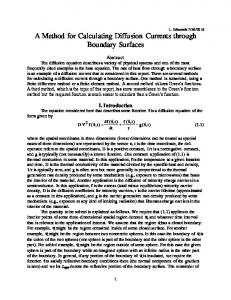
3. Basis functions for cracklet opening displacements As stated, our solution strategy begins with a decomposition of the array of cracks into a convenient set of n straight cracklets, typically extending from crack tips to kinks or branch points, or between such points (though further subdivision of long cracklets may prove desirable under some circumstances). The task in this section is to determine the ‘correct’ functional form of the ODPs for the cracklets, from which we may obtain the dislocation density pair (i) (µ(i) 1 (t), µ2 (t)) for each cracklet (i.e., each C i ) by taking derivatives with respect to the position parameter t along the cracklet line, and including delta functions to reflect any jumps at the ends. For illustration we consider a single crack with several kinks, partitioned into n straight cracklets of differing orientations, as shown in Figure 2. We must find functions to describe, self-consistently, the cracklet ODPs and singular field behavior induced, such that the residual part (leaving only physically realistic singularities in the material), can be determined easily in analytical terms. 3.1. K EY

ISSUES IN WEDGE ANALYSIS AND MATERIAL DISTORTION

The most important and obvious features where cracklets join are the jumps in cracklet opening displacements that occur at kinks and branch points where material wedges exist. As mentioned, these jumps produce delta functions in the cracklet dislocation density pairs, and these produce inverse-of-distance singularities in their induced monotractions and monostresses at cracklet end points. By properly matching jumps for adjacent cracklets, these singularities will cancel in both the net tractions and the resulting stress fields. Less obvious is the role of slope components of the ODPs at cracklet joints, whereby the dislocation density pairs approach constant values. These produce log-distance singularities in

Superposition method for calculating singular stress fields 109

Figure 2. A single kinked crack made up of n straight cracklets. Local interactions between two adjoining cracklets of kink angle ω are studied by considering two associated wedge problems in polar coordinates, shown in the inset.

the induced monostresses and monotractions, which should also cancel in the superposition. Intuitively, one might suspect that properly relating these ODP slopes at a kink or branch reflects in plane rotation of one wedge relative to another. In the auxiliary problem, however, this is an oversimplification as becomes apparent when one attempts to appreciate the subtle conditions (Appendix B) under which the log singularities can cancel in the net tractions, as must physically occur. In fact, one can arrange for such singularities to cancel, yet fail to allow the natural rotation or displacement of one wedge with respect to its mate, thus generating spurious local tractions and distorting the true stress field in the material. Even less obvious is the representation of any wedge tip singularities (1/2 < λ < 1) at kinks and branches and how these are reflected in the cracklet ODPs. These singularities should cancel in the net tractions but the stress singularities should remain in the material. These also have generalized SIFs worthy of evaluation, yet to our knowledge this aspect has been neglected. Proper handling of all of these ODP features, necessitates careful study of the singular behavior occurring at kinks and branches. The singular part of the interaction between adjacent cracklets at a kink is found by studying the associated wedge problems for the upper and lower crack faces, following Williams (1952). In Figure 2, the interaction between the two cracklets with included angle ω < π is revealed by considering the upper and lower wedges of angles ω and 2π − ω, as shown in the inset. It turns out to be simplest to develop the local wedge analysis in terms of the original problem where the boundaries of both wedges are traction-

110 J. Kenneth Burton Jr. and S. Leigh Phoenix free near the vertex, rather than in terms of in the auxiliary problem where the upper and lower wedge faces have constant tractions ±τ . The crack opening displacements as well as the cracklet ODPs will be the same in both problems, as they should be. Note, however, that the local stresses will differ by the constant stress σ ∞ in the trivial problem. More subtly, the displacement fields will also differ because the uniform stretching and Poisson contraction in the trivial problem (without cracks) causes angle distortions of the crack lines, and thus, of the local wedge angles in the auxiliary problem that do not occur in the original problem. Alternatively, in the analysis of the wedges, one may think of these distortions as being caused by the tractions ±τ , which do not create log singularities since no log singularities occur at these material positions in the trivial problem. In superimposing the stress fields of adjacent cracklets, the key to achieving the correct local behavior is to develop natural constraints on local deformation that fully allow the appropriate local wedge distortion, including translation and rotation, yet ruling out singularities in the net tractions after superposition. This is a nontrivial task, which is carried out in Appendix B. 3.2. C RACKLET

SINGULAR BEHAVIOR AND INTERACTIONS FROM WEDGE ANALYSIS AT KINKS AND BRANCHES

Following the analysis of Williams (1952) for traction free wedges, and using the polar coordinate system shown in Figure 2, the crack opening displacement 1u(r, θ) at a kink can be written as a difference of displacements for the upper and lower wedges resulting in the form X 1u(r, θ) ≈ cλ (θ)r λ , (9) λ

where cλ (θ) is a coefficient, and the sum ranges over λ satisfying either the eigenvalue Equation sin(λω) = ±λ sin(ω),

(10)

for the upper wedge, or sin(λ(2π − ω)) = ±λ sin(ω),

(11)

for the lower wedge, and where r is distance along the wedge faces from the vertex. Dependence of cλ on angle θ denotes the fact that this coefficient in general differs for two adjoining cracklets. Also 1u and cλ are both vectors with tangential and normal components. Continuity and boundedness of the displacements for each wedge requires that only eigenvalues λ > 0 be considered, and singular monotractions arise for terms with 0 6 λ 6 1, the special case λ = 1/2 being an exception. (Corresponding to an opening displacement of the form r λ , where λ is not an integer, the leading asymptotic behavior of the monotraction as r → 0 is proportional to cot(π λ)r λ−1 + const. The coefficient of the first term vanishes when λ is an odd half-integer.) Equations (10) and (11) both have λ = 0 and λ = 1 as eigenvalues allowing, respectively, translation and rotation of one wedge relative to the other. Since (10) for the upper wedge has material angle ω < π there are no real solutions with 0 < λ < 1, implying there will be no singular stresses in the upper wedge. The remaining singular behavior comes from the solutions to (11) for the lower wedge, corresponding ultimately to the singular stress behavior in the lower wedge material. Equation (11) has no real solutions, 0 < λ 6 1/2, and exactly one or two such solutions, 1/2 < λ < 1, depending on ω. Only one solution occurs when ω > ωc = 1.7898 radians (102.55 degrees), but two real solutions

Superposition method for calculating singular stress fields 111 occur for ω < ωc . The smallest eigenvalue λ = ρ1 , where 1/2 < ρ1 < 1, produces the strongest singular stress behavior for the lower wedge and symmetric (mode I) deformation with respect to the wedge angle bisector. When a second such eigenvalue λ = ρ2 exists, it satisfies 1/2 < ρ1 < ρ2 < 1 and produces singular stresses with antisymmetric (mode II) deformation. Thus, there are either three or four ‘singular’ terms that should appear in an expansion of the opening displacement, Equation (9), near the kink vertex. These should be reflected in the ODP basis terms for the adjoining cracklets. It is important to point out that although ρ1 is less than ρ2 , and thus, corresponds to the leading singular behavior of the lower wedge, this is not justification for ignoring terms associated with ρ2 . Doing so artificially prevents physically reasonable mode II singular distortion of the lower wedge, thus eliminating one possible cause for crack branching in applications. There may also be complex solutions to (10) and (11), but these have real parts greater than 1. Thus, while they produce material stresses that oscillate infinite rapidly near the wedge vertex, these stresses are bounded by functions approaching zero as r → 0. Leaving out these oscillatory terms does not result in net tractions (after superposition) that are singular or oscillatory, and in fact, these tractions remain well-behaved. (For example, in the auxiliary problem constant tractions produce these same oscillations.) Terms in (9) with the correct λ (or ρ) power are essential to avoid singular net tractions while reflecting the appropriate singular material behavior, but there is no such need for the nonsingular terms. In developing higher order basis terms for more refined corrections to the opening displacements, the function space spanned by the ‘correct’ (by wedge theory) nonsingular terms is also spanned by other basis choices, meaning that the nonsingular part of the material stress field will be represented accurately. So long as efficiency in converging to the solution is not compromised, any convenient basis set may be chosen and we will make a particular choice. Thus, by developing an efficient basis set, the correct stresses and displacements within the material can be approximated accurately. The same ideas apply to interacting, joining cracklets representing say k > 2 crack branches emanating from a point. In this case, k wedge problems arise rather than just two, with k distinct angles summing to 2π , and we can write k eigenvalue equations in place of (10) and (11). Singular behavior within the material will occur only for a wedge whose material angle is greater than π , and there can be at most one. The exponents can again be taken as λ = ρ1 and ρ2 (if such occurs), and we will have singular solutions for these ρ values, and thus, singular behavior captured by (9) for the two cracklets adjacent to this wedge. For an isolated cracklet tip at the end of a crack, the monotraction does not diverge. We can write the opening displacement as in (9) with ω = 0, but without θ-dependence. The only value of λ that generates a divergent material stress field, but a bounded monotraction, is the usual 1/2 associated with the square-root singularity. 3.3. BASIS

FUNCTIONS FOR CRACKLET OPENING DISPLACEMENT PROFILES

We now construct sets of basis functions for cracklet ODPs, some of which produce special opening shapes to reflect the local behavior at crack kinks and isolated tips, and others of which allow finer corrections. These sets allow great flexibility in representing possible opening displacements for the system of cracks upon taking a weighted sum of relatively few terms for each cracklet. The same basis sets will serve for both normal and tangential opening displacements, independently. The members of each set are constructed so that the stress and displacement fields, and induced crack line monotractions can be evaluated analytically,


Figure 3. Normal opening shapes generated by basis functions in Tkink and Ttip where the tip corresponds to the right end. Those for Ikink,1 are the same as those for Tkink except the fundamental shape is a rectangle. Those for Ikink,2 are those for Ikink,1 rotated π radians. Corresponding tangential opening shapes are not shown.

using methods given in Appendix A (where irrational singularity exponents are replaced by arbitrarily close rational approximations). This eliminates the possibility of errors arising from numerical integration, and permits simpler error estimates. We build two fundamental basis sets: The first set applies to what we call terminal cracklets, that is, where the cracklet begins at a crack kink or branch (or subdivision point), and ends at a crack tip. The second set applies to interior cracklets, where each end is either at a kink, a branch, or a subdivision point. First we consider a terminal cracklet of length a, where the right end corresponds to a crack tip, and distance r is measured from the left end corresponding to a kink of angle ω 6 = π or a crack subdivision point of angle ω = π (a degenerate kink). When 0 < ω < ωc we let {ρ1 , ρ2 , 1} be the set of singularity exponents for the kink. (We do not include 0, though it is accommodated later.) When ω > ωc we label the only such solution ρ1 , and have the set {ρ1 , 1}. For ω = π we have only the set {1}. We define basis ODPs consisting of a fundamental function and two sets of correction functions with asymptotic power behavior in terms of distance from either cracklet end, as motivated by the singular wedge or tip behavior described by (9). For a terminal cracklet, our fundamental basis function is the semiellipse, e(r, a), given by e(r, a) = {1 − (r/a)2 }1/2 ,

0 6 r 6 a,

(12)

as illustrated in Figure 3. It generates the usual square-root singularity in the stress field around the tip and a 1/r singularity in both the material and the monotraction at the kink end, but no log r singularity since the slope approaches zero. A cracklet ODP will have this shape (with tangential and normal components) if it is the right half of an isolated crack in an infinite body loaded uniformly in the far field. Generally the left end in (12) will not capture the wedge features in (9) at a kink, so we must create additional basis correction functions or ODPs.

Superposition method for calculating singular stress fields 113 The first set of basis correction functions, Tkink, consists of kink corrections given by Tkink = {r nρ (1 − (r/a)ρ )2 : n ∈ W, ρ ∈ {ρ1 , ρ2 , 1} or {ρ1 , 1} or {1}, depending on ω},

(13)

where W = {0, 1, 2, 3, . . . } and 0 6 r 6 a. (We define the basis functions with only ‘partial’ normalizations in order to simplify the discussion in Appendix B.) Each correction function in Tkink dies out as the square of the distance a − r to the tip, thus causing no stress singularity there. When n = 0, 1, 2, . . . we call the corresponding functions, kink correction functions of the ‘zeroth order’, ‘first order’, ‘second order’, etc. When ρ is 1, we call the corresponding functions ‘polynomial’ kink correction functions, and when ρ is ρ1 or ρ2 , we call them ‘wedge’ kink correction functions. This distinction is important because polynomial kink correction functions do not ultimately produce material stress singularities unlike their wedge counterparts. The normal components of the cracklet opening shapes created by the various basis functions (in isolation) are shown in Figure 3. Note that the zeroth order polynomial corrections have a step opening as well as a nonzero slope at the kink end (r = 0), generating 1/r and log r singularities, respectively, in both the material stresses and the monotractions. The first order polynomial corrections have no step opening but a nonzero slope generating log r singularities. The zeroth order, wedge corrections also have a step opening at the kink, and both the zeroth and first order wedge corrections contribute local r ρ opening displacement behavior there, which ultimately generates the r ρ−1 singular stress behavior in the material. The second set of basis correction functions, Ttip , consists of tip shape corrections given by Ttip = {(r 0 )n+3/2 (1 − (r 0 /a)1/2 )2 : n ∈ W },

0 6 r 0 6 a,

(14)

where r 0 = a − r is distance from the tip end. Each function in Ttip dies out as the square of the distance r from the kink end, causing no singularity there. When n = 0, 1, 2, . . . , we call the corresponding basis functions, tip correction functions of the ‘zeroth order’, ‘first order’, ‘second order’, . . . . The normal cracklet opening shapes created by these tip corrections (in isolation) are shown in Figure 3, where the right end corresponds to the tip. The nth order correction function dies out as the power n+3/2 of the distance r 0 from the tip, thus generating no singularity. Note that n + 3/2 is a natural eigenvalue for a wedge of angle 2π (a crack). These correction √ functions create local tip distortions similar to those for an ellipse multiplied by (a − r)n+1 a/2. The full basis set for terminal cracklets is T = {e(r, a)} ∪ Tkink ∪ Ttip. Essentially we model a terminal cracklet ODP as the vector function X X 1uT (r) = ce(r, a) + cknρ fknρ (r, a) + ctn ftn(r, a), (15) n,ρ

n

where functions fknρ (r, a) and ftn (r, a) are taken from basis Tkink and Ttip , respectively, and the weights c, cknρ and ctn are vectors, with tangential and normal components. When the left end of a terminal cracklet corresponds to a branch point with flanking material wedges of angle ω0 and ω00 , respectively, singular behavior must be considered only if the larger angle exceeds π . Then we use the above basis sets with ρ ∈ {ρ1 , ρ2 , 1} or {ρ1, 1} from the larger angle depending on its value. If neither ω0 nor ω00 exceeds π , we may take ρ ∈ {1}, since no singular material stress behavior occurs. Alternatively, we may arbitrarily choose ρ

114 J. Kenneth Burton Jr. and S. Leigh Phoenix to be a convenient fraction between 1/2 and 1 and construct the basis set as above but requiring the r ρ terms to cancel. Later we consider a star-shaped crack, obtaining fast convergence for ρ = 2/3. Next we consider basis functions for an interior cracklet of length a, which spans between two kink points designated ‘1’ and ‘2’ at the left and right ends, with kink angles ω1 and ω2 , respectively. We let ri be distance measured along the cracklet from kink i, so r2 = a − r1 . We also let {ρ1i , ρ2i , 1} or {ρ1i , 1} be the sets of singularity exponents for the largest wedge at kink i, depending on the value ωi relative to ωc (or take {1} if ωi = π ). The fundamental basis function for an interior cracklet is the constant, {1}, representing a rectangular ODP (Figure 3). It generates 1/ri type singularities at the respective ends, but no log ri singularities. The two sets of basis correction functions are Ikink,1 and Ikink,2 consisting of shape correction functions for kinks 1 and 2, respectively. These are Ikink,i = {rinρ (1 − (ri /a)ρ )2 : n ∈ W, ρ ∈ {ρ1i , ρ2i , 1} or {ρ1i , 1} or {1}, depending on ω},

i = 1, 2.

(16)

Each correction function in Ikink,i dies out as the square of the distance ri − a to the opposite end, thus causing no stress singularity there. When n = 0, 1, 2, . . . we call the corresponding functions, kink correction functions of the ‘zeroth order’, ‘first order’, ‘second order’, and so on. When ρ is 1, we refer to the corresponding functions as ‘polynomial’ kink correction functions, and when ρ is ρ1i or ρ2i we refer to them as ‘wedge’ kink correction functions. The correction functions in Ikink,i have properties at kink end i that are the same as those described for Tkink. The normal cracklet opening shapes created by these kink corrections (in isolation) are shown in Figure 3. (Analogous tangential versions exist but are not shown.) In the superposition those for i = 2 would be those for i = 1 rotated π radians. When an end, i, of an interior cracklet corresponds to a branch point, we modify the basis set just as we did with Tkink . The full basis set for an interior cracklet is thus I = {1} ∪ Ikink,1 ∪ Ikink,2. Essentially we model it’s ODP, expressed arbitrarily in terms of distance r1 from kink 1, as the vector X X 1uI (r1 ) = d + d 1nρ g1nρ (r1 , a) + d 2nρ g2nρ (a − r1 , a), (17) n,ρ

n,ρ

where functions g1nρ (r1 , a) and g2nρ (r2 , a) are from basis sets Ikink,1 and Ikink,2, respectively, and the weights d, d 1nρ and d 2nρ are vectors, with tangential and normal components. The case of straight cracks with neighbors is special. Such a crack of length 2a may be considered as two adjoining, terminal cracklets, with kink angle ω = π, ρ ∈ {1}. An alternative, is to take the function e(r, a) extended over −a 6 r 6 a to become an ellipse, 0 and use the right tip correction basis set, Ttip (r) obtained from Ttip(r) by replacing a with 2a 0 in the denominator of the fraction in (14), as well the ‘reflected’ basis set Ttip (−r) for the left tip. These sets up to order n are not the same as the basis formed by multiplying an ellipse by a polynomial or order n. 3.4. E VALUATION

OF CRACKLET MONOSTRESS AND MONODISPLACEMENT FIELDS

In summary, the normal and tangential opening displacements of each interior and terminal cracklet, ‘in isolation’, are modeled as weighted sums of basis functions that produce opening shapes as shown in Figure 3 (which shows only normal versions). Some normal weights

Superposition method for calculating singular stress fields 115 may be negative yet the overall normal opening displacements may be positive. The opening displacements for the system of cracks are created by assembling the sequence of opening displacements of the individual cracklets C i along C, joining them together at kinks and branch points. Note that center-line distortions of the resulting opening shapes will result when the cracklets mutually interact after superposition, but the opening displacements will be unaffected. To determine the monostress and monodisplacement fields induced by the basis functions in sets T and I , note that each function in Tkink, Ttip and Ikink,i has an expansion in terms of distance r(or r 0 or ri ) from a cracklet end of the form a nρ (r/a)nρ − 2a nρ (r/a)(n+1)ρ + a nρ (r/a)(n+2)ρ over 0 6 r 6 a, for some integer n > 0 and 1/2 6 ρ 6 1. Integrals required to determine the monostress and monodisplacement fields due to the opening displacements e(r, a) and those of the form r nρ over 0 6 r 6 a are given in Appendix A, where particular attention is paid to singularities produced at r = 0 and r = a due to any jumps and slope changes there. 4. Solution strategy, constraints and estimating error In solving a multi-crack, auxiliary problem, the key task is to find crack opening displacements (i) in terms of the cracklet ODPs and dislocation density pairs (µ(i) 1 , µ2 ) that generate net crack tractions (after superposition) that very closely satisfy the traction balance Equations (8a, b), together with (3) and (4). An exact series solution, would involve an infinite, weighted sum of basis terms for each cracklet, but in practise we want high accuracy with as few terms as possible. We can then calculate the auxiliary problem stresses σxx , σyy , and σxy for the body using (3)–(6), and analogously the material displacements u1 and u2 , using results in Appendix A. The full solution requires adding to these the stresses and displacements from the trivial problem. 4.1. L EAST

SQUARES CALCULATION OF COEFFICIENTS , ALLOCATING POINTS , AND ESTIMATING ERROR

Summing over all cracklets, we suppose there are a total of 2m basis terms being used (m normal and m tangential) so that 2m equations are needed to solve for the unknown weighting coefficients. Instead of picking m points along the cracklets according some spacing rule, and enforcing Equations (8a, b) at each point, we consider M > m points and perform a least squares fit. This allows extra weight to be given to important regions of the overall crack line, especially when few DOF are being used (unlike numerical quadrature methods, where the points are fairly rigidly determined by the number of DOF). If one is interested primarily in crack tip SIFs, one may allocate a higher density of points near crack tips to enhance accuracy there. A simple rule to locate M 0 points along a terminal cracklet of length a is to choose points rj , j = 1, . . . , M 0 measured from the kink end according to rj /a = sin{j π/(2M 0 + 2)}. For interior cracklets of length a, M 0 points can be equi-spaced. This method, however, can yield slow convergence for the generalized SIFs for wedge singularities at kinks, especially when both symmetric ρ1 and antisymmetric ρ2 singular deformation modes are present. Thus, to give added weight near kink singularities, one can split up the points and use the above rule at both ends of the cracklet. In later calculations this approach works better. Measuring the tractions at more than the minimum number of points also allows us to make error estimates. Dividing the least squares error of the fit by the sum of the squared normal

116 J. Kenneth Burton Jr. and S. Leigh Phoenix and tangential prescribed tractions, and taking the square root, gives an order-of-magnitude estimate of the relative error in the net crack face tractions and the calculated stress field. We refer to these estimates as relative root mean square (RRMS) error estimates. We will also calculate errors in the SIFs as compared to stable or known values.

4.2. NATURAL

CONSTRAINTS ON SINGULAR BEHAVIOR AND IMPLICATIONS

As mentioned, divergent monotractions are produced by certain basis ODPs that produce singular basis fields. Handling them improperly can lead to errors despite choosing many points close to where cracklets join (and despite apparent decreasing error with increasing m). To avoid this difficulty, we apply certain natural constraints on the leading asymptotic behavior of these singular monotraction terms where cracklets join, so that all traction singularities cancel out automatically. (The tractions become prescribed constants in the auxiliary problem.) Developed in Appendix B, these constraints produce certain algebraic relationships among basis function coefficients, depending subtly on the kink angle ω, and they also reduce the DOF. Similar constraints arise at a branch, the number depending on whether or not adjacent cracklets create a wedge with material angle ω0 > π . These constraints have implications in using certain basis terms: At a kink, the ODP terms e(r, a) and {1 − (r/a)ρ }2 in basis set T , and corresponding terms in set I approach 1 as r → 0 representing jump discontinuities (Figure 3). Thus, each produces a 1/r monotraction singularity, as shown in Appendix B. In the superposition, requiring that these singularities cancel adds two constraints relating the respective coefficients used for tangential and normal opening displacements of adjoining cracklets. Physically this behavior corresponds to the λ = 0 eigenvalue in (10) and (11), which allows translation of one wedge relative to the other. The functions {1−(r/a)ρ }2 and r ρ {1−(r/a)ρ }2 in T and corresponding functions in I each contribute an ODP term proportional to r ρ (Figure 3). Requiring that the induced singularities cancel (in the net tractions but not in the material) adds constraints relating the coefficients of tangential and normal opening displacements of these terms, respectively. When 1/2 < ρ < 1, three constraints arise at a kink, leaving only one independent coefficient, which we later relate to the SIF for either mode I or mode II deformation for the r ρ−1 wedge singularity. For ρ = 1, three constraints arise, provided that ω is not a multiple of π/2, in which case only two arise. When three arise, the one adjustable coefficient remaining allows rotation of one wedge relative to the other. When ω = π through a joint, the upper and lower crack surfaces can rotate with respect to one another, but also, one surface can be uniformly stretched tangentially relative to the other. For the cases ω = π/2, or ω = 3π/2, an angle increase between the crack surfaces on one side must be compensated by an angle decrease by the same amount on the other (rotation), but tangential sliding and stretching displacements of the mating crack surfaces relative to each other, locally proportional to r, is also possible. On the two faces of a wedge, the surface stretching will have opposite signs, giving rise to antisymmetric distortions within each wedge relative to its bisector. These constraints are consistent with requiring that the material wedge angle distortions be zero in the original problem (where the crack face tractions are zero), though not generally in the auxiliary problem because angle changes are needed to compensate for uniform shear strain distortions in the material (depending on Poisson’s ratio) added from the trivial problem. Note that if exponent ρ were not chosen to satisfy (11), the constraints on the associated coefficients would force them all to be zero!

Superposition method for calculating singular stress fields 117 4.3. O RDER

OF CHOOSING BASIS FUNCTIONS IN IMPROVING ACCURACY

Generally we start with the semiellipse terms for tip cracklets and rectangular openings for interior cracklets, and then add zeroth order polynomial and wedge kink corrections. Since the zeroth order kink corrections in T and I actually expand to give ‘first order’ terms proportional to r ρ , using them alone requires applying the constraints in Appendix B to null out the singularities, thus reducing the DOF. To make all four DOF available at this stage, but at the same time not providing wedge singularity or rotation corrections, we add compensating first order (n = 1) correction terms ‘parasitically’ to null out the singularity produced by each term. Next we add zeroth order tip corrections. Then we add first order kink (wedge then polynomial) corrections; at this stage wedge singularities and wedge rotation become possible, reducing errors dramatically. After that are first order tip correction terms, followed by second order kink corrections, and so on. This cycle seems to work well as a ‘rule-ofthumb’. When crack tips are not mutually close, tip correction terms often have little effect on the convergence, so delaying their use is reasonable. 5. Stress intensity factors for crack tips, and kink and branch singularities For the crack tips, the SIFs, KI and KII , are obtained from the coefficients of the elliptical basis terms e(r, a) for opening and tangential displacements respectively, since these determine the curvatures of the openings at the crack tips. This leads to the well known result 2G p (KII , KI ) = c π/a. (18) 1+κ For a kink, we consider the wedge with the largest material angle, say ω0 = 2π − ω, and recall that the zeroth and first order wedge correction terms, of the form {1 − (r/a)ρ }2 and r ρ {1 − (r/a)ρ }2 both contribute to the local opening displacements (between the wedges) of the form r ρ causing the singular stress behavior in the material. Expanding these functions and collecting like terms gives opening displacements between the two wedge mating surfaces radially outward in both directions of the form 1uρ (r) ≈ (ck1ρ − 2ck0ρ )r ρ ,

(19)

(where c may be d depending on cracklet type). For ρ = ρ1 an ‘opening’ mode occurs producing symmetric mode I deformation; the normal opening components of the displacements are the same for the two wedge surfaces, and a positive constant c2 or d2 corresponds to a positive stress intensity factor, with positive normal opening displacements on each side and radially positive (outward directed) wedge surface displacements relative to the apex. This requires the tangential c1 or d1 components to be opposite from one wedge side to the other (see Appendix B). Note that the surface of the wedge with the smaller material angle, ω, does not ‘absorb’ these opening displacements because ρ1 is not an eigenvalue for that wedge. For ρ = ρ2 we have antisymmetric mode II deformation; the opening components of displacements c2 or d2 are equal but opposite from one surface to the other, but the c1 or d1 components are the same (causing opposite radial wedge surface displacements; see Appendix B). We can calculate the generalized SIFs, KI(ρ1 ) and KII(ρ2 ) corresponding to these two deformation modes, respectively, by studying the relationship between the singular stress along the wedge angle bisector (normal in mode I, and shear in mode II) and the wedge surface displacements caused by the opening displacements from these basis terms. For mode I, we may write

118 J. Kenneth Burton Jr. and S. Leigh Phoenix the normal stress along the wedge bisector at angle θ 0 = π − ω/2 as σθθ = KI(ρ1 ) /(2π r)1−ρ1 . For mode II, the corresponding shear stress is of the form τrθ = KII(ρ1 ) /(2π r)1−ρ2 . Using results in Appendices A and B (or working directly with the results of Williams (1952)) we calculate 2G (ρ1 − 1) sin[(ρ1 − 1)ω0 /2] (ρ1 ) 1−ρ1 KI = − ρ1 (ρ1 + 1) 1 − (2π ) 1+κ (ρ1 + 1) sin[(ρ1 + 1)ω0 /2] × and KII(ρ2 )

c2k1ρ1 − 2c2k0ρ1 , sin[(ρ1 − 1)ω0 /2]

(20)

2G sin[(ρ2 − 1)ω0 /2] ρ2 − 1 1−ρ2 = − ρ2 (ρ2 + 1) (2π ) − 1+κ sin[(ρ2 + 1)ω0 /2] ρ2 + 1 ×

c1k1ρ2 − 2c1k0ρ2 , sin[(ρ2 − 1)ω0 /2]

(21)

where ω0 = 2π − ω, c2 · corresponds to normal and c1 · to tangential opening displacements. These result can be shown to collapse to the usual stress intensity factors for crack tips when ω0 = 2π and ρ = 1/2. In the case of interior cracklets c becomes d. (Appendix B uses d in the notation.) 6. Example problems and solutions We now consider several examples to illustrate the power of the method. Specifically, we investigate the ability of various basis terms to eliminate error, which will be given in relative terms as both the estimated RRMS error in the net tractions and relative error in the SIFs, as compared to known or stable values. Some examples have certain symmetries in crack geometry and loading, but to better appreciate the DOF requirements under arbitrary loading, we do not take advantage of these symmetries in the calculations. Also, the DOF represent the number of terms used minus the constraints on the weight coefficients (Appendix B). This is the number of rows in the matrix to be inverted in the least squares fit, which is the main rate-determining part of the algorithm. 6.1. A NGLED

CRACK OF EQUAL - LENGTH ARMS

Consider first a kinked crack with two equal, arms of length a = 1 and kink angle ω = 2π/3, which is modeled as two terminal cracklets as shown in Figure 4. In the original problem the applied, far-field load is simple unit tension along the crack mirror line. The basis set used is T , where for ω = 2π/3, ρ1 = 0.61573 is the only solution of (11) between 0 and 1. We use its rational approximation 8/13, accurate to within 0.06 percent. The number of points chosen for the least squares fit was 19 per cracklet. The density of points was increased near the crack tip according to the method in Section 4.1, but not near the kink where the first point appeared at r/a = 0.0785. The net tractions obtained by doing a least squares fit with various DOF, are shown in Figure 5 along with estimated crack-tip SIFs. Table 1 lists these SIFs along with the RRMS error estimates (as percentages) in the net tractions and calculated SIF errors (as compared to


Figure 4. An angled crack in an infinite plate shown as two terminal cracklets of length a and forming a kink of angle ω. The actual case treated has ω = 2π/3 and a = 1. The loading in the original problem is uniform, far-field tension along the mirror symmetry line. Table 1. Calculated SIFs versus DOF for the 2π/3 angled crack problem. Also shown are SIF errors (compared to 44 DOF) and corresponding RRMS errors in the net tractions. DOF

KI

KII

RRMS error

2 6 6 15 15 20 44

1.275030 (+1.6%) 1.248647 (−0.5%) 1.241887 (−1.0%) 1.252701 (−0.17%) 1.254522 (−0.023%) 1.254717 (−0.0081%) 1.254817

0.736139 (−13%) 0.813483 (−3.8%) 0.842789 (−0.3%) 0.837699 (−0.93%) 0.845439 (−0.017%) 0.845506 (−0.0099%) 0.845590

15.0% 11.5% 8.6% 5.6% 0.44% 0.093% 3 × 10−5 %

values at 44 DOF). Note the absence of any singularities or cusps in the net traction plots on Figure 5, where for the maximum, 44 DOF, the estimated RRMS error in the net traction is only 3 × 10−5 percent. The case of 2 DOF uses just the semiellipse basis terms for normal and tangential openings (4 DOF minus 2 constraints to avoid 1/r stress and traction singularities). Already the errors in the SIFs are surprisingly small. For the 6 DOF cases we add either zeroth order polynomial corrections (ρ = 1) or zeroth order wedge corrections (ρ1 = 8/13) (together with parasitic first order corrections to suppress singularities yet allow the 2 added DOF each). In either case the four additional DOF allow the local curvature at the crack tips and the opening displacements at the kink to be adjusted independently. Adding these terms does not yet permit wedge singular distortions. In Figure 5(a) we note that these correction terms each give qualitatively similar improvements. To get the two cases of 15 DOF, we add both zeroth order wedge and polynomial terms (adding 4 each), zeroth order tip corrections (adding 4 more), and either first order wedge or first order polynomial corrections (adding 1 more each after satisfying constraints). In Figure 5(b) the performance is much better in the case of wedge corrections versus polynomial corrections (0.44 percent versus 5.6 percent RRMS error). Because of the symmetry of the loading and geometry, there is actually no need for first order polynomial corrections, which correspond to rotation of one wedge relative to the other, but the wedge correction


(a)

(b) Figure 5. Net normal and shear tractions in the auxiliary, angled crack problem (ω = 2π/3) with prescribed (target) tractions derived from the original problem: (a) cases with elementary and zeroth order basis terms; (b) cases with first order kink and zeroth order tip correction terms, and higher.

corresponding to symmetric mode I, singular distortions in the lower wedge is needed. With more general loading, both terms will be needed. For larger numbers of DOF (20 by adding in first order tip correction terms, and 44 all the way up to third order) the net traction profiles (Figure 5(b)), are virtually indistinguishable from the prescribed tractions. Indeed most of the visible improvement has occurred by 16 DOF. The tip correction terms have relatively little effect when added, but may be important when considering closely spaced tips. The wedge generalized stress intensity factor KI(ρ1 ) was calculated from (20) to be −0.449 at 44 DOF, meaning the wedge is in a symmetric closing mode (though without surface interference since the wedges are separated). Just before adding the wedge corrections (second

Superposition method for calculating singular stress fields 121 15 DOF plot) the traction plots show that, to suppress the singularity, the residual tractions (net minus prescribed) must force the lower wedge open through local surface shear tractions directed outward from the tip. At 15 DOF, when the wedge correction was first added, KI(ρ1 ) was calculated to have the value −0.443, which differs by less than 1.5 percent from that at 44 DOF. However, the fact that calculation points were relatively sparse near the kink, caused fluctuations for DOF choices between 15 and 28 that were up to 4 percent different. We believe the final value is accurate to 1 percent. The errors in the crack-tip SIF are all much less (sometimes by an order of magnitude) than what is suggested by the RRMS error, suggesting that the RRMS error provides a good estimate for the relative error in the solution. On the other hand, these RRMS error estimates are probably lower than what would be calculated by having a higher density of points near the wedge tip, which would capture more realistically local fluctuations in the net tractions. The apparent high accuracy obtained in the crack-tip SIFs occurs because these local fluctuations tend to average out. 6.2. S INGLE

STRAIGHT CRACK SUBDIVIDED INTO MULTIPLE CRACKLETS

To obtain insight into what happens when we break up long straight crack segments into cracklets, we consider a single crack of length 2a = 2, subdivided into two and three cracklets, respectively. There are no kinks at the cracklet junctions, so the wedge angles are both π , and there are no ρ values less than 1. For a straight crack, a unit, remote tensile loading at arbitrary angle can be decomposed into remote tension perpendicular to the crack line and remote tangential shear, both with known solutions. Also, normal and transverse cracklet ODPs generate normal and tangential monotractions, respectively. Thus we consider only a unit normal load (though the DOF requirements reflect those for arbitrary loading angle). Note that viewing this crack as two adjoining cracklets of equal length a turns out to be trivial, since taking the semiellipse basis term e(r, a) for each component and applying the constraint leaves 2 DOF, which allows matching to the net tractions exactly, thus leaving the well known crack solution. We first view the single crack as two terminal cracklets of unequal length a1 = 1.2 and a2 = 0.8 (see Figure 6(a)). The net traction obtained with various DOF is shown in Figure 6. Table 2 gives the SIF estimates and errors, and the RRMS error for the net tractions. The number of calculation points along each cracklet was again 19 with increased density only at the crack tips. For just 2 DOF we use 2 normal and 2 tangential opening semiellipses e(r, a) with the two constraints. This prevents us from independently varying the opening curvature at each tip, resulting in bulging on the right. Adding 4 more DOF through zeroth order polynomial corrections (but with first order compensation to prevent log r singularities in the tractions), allows varying the curvature of each crack tip without allowing the local slope of the ODP at the joint to deviate from horizontal (no rotation or kink in the ODP) or upper and lower surfaces to stretch relative to each other (though this does not occur for this particular loading). Adding 4 more DOF using zeroth order tip corrections, yields only a slight improvement, but when we add first order polynomial corrections together with the two constraints (to prevent log r traction singularities) yielding 12 DOF in total, the slope of the ODP at the joint adjusts and the error reduction is dramatic. Further alternating between tip and polynomial corrections yields further improvements, and again the RRMS error estimate seems conservative relative to that for the SIFs.


Figure 6. Net normal tractions in the auxiliary problem of a single straight crack of length 2a = 2 originally under far-field tension, when viewed as (a) two unequal cracklets, and (b) three cracklets (see insets). Table 2. Calculated SIFs versus DOF for a straight crack modeled as two unequal-length cracklets. Also shown are SIF errors and corresponding RRMS errors in the net tractions. DOF

√ KI1 / π

√ KI2 / π

RRMS error

2 6 10 12 24

0.864981 (−13.5%) 0.985112 (−1.5%) 0.986086 (−1.4%) 0.999991 (−0.0009%) 1.000000 (+4.1 × 10−5 %)

1.059380 (+5.9%) 0.997792 (−0.2%) 0.999174 (−0.08%) 1.000013 (+0.0013%) 1.000000 (+3.6 × 10−5 %)

14.5% 5.8% 5.3% 0.12% 0.005%

Superposition method for calculating singular stress fields 123 Table 3. Calculated SIFs versus DOF for a straight crack modeled as three cracklets. Also shown are SIF errors and corresponding RRMS errors in the net tractions. DOF

√ KI / π

RRMS error

2 10 14 18 54

1.031475 (+3.1%) 1.017797 (+1.8%) 1.016595 (+1.65%) 1.000002 (0.0002%) 1.000000 (+1.9 × 10−5 %)

17.0% 10.5% 10.0% 0.195% 1.4 × 10−5 %

In the second case we view the above single crack as three adjoining cracklets, two terminal ones of length 0.75, and an interior one of length 0.5 (see Figure 6(b)). The net tractions obtained for various cases up to 54 DOF are shown in Figure 6(b). Table 3 gives estimates of the SIFs and the various errors. For 2 DOF we use opening and shear semiellipses for the terminal cracklet (from T ) and opening and shear rectangles for the interior cracklet (from I ). The flattening effect of the rectangle produces the anticipated errors. Adding zeroth order polynomial corrections (with first order compensation) at the two joints (4 DOF each) and zeroth order tip corrections (4 DOF) does not reduce the error substantially. Adding first order polynomial corrections (2 more DOF at each joint) to get 18 DOF allows adjusting the local ODP slopes, dramatically improving accuracy. Again, the RRMS error seems to provide a conservative estimate of the actual errors. These two examples demonstrate the need for certain basis corrections at the cracklet joints, especially first order polynomial corrections. They also strongly suggest that subdividing straight cracks or cracklets into several smaller cracklets is typically an efficient way to allocate DOF, and that it is better to add higher order basis terms over the full length between true kinks or tips. 6.3. C RACK

WITH TWO KINKS

A more challenging example is a crack with two kinks, modeled as two terminal cracklets and one interior cracklet, as shown in Figure 7. We consider the case a1 = a2 = a3 = 1, with kink angles φ1 = 5π/3, and φ2 = 2π/3, and with a unit, remote tensile loading applied parallel to the axis of the middle cracklet. For kinks i = 1, 2, the wedges have angles φi and 2π − φi , respectively, and the wedge singularity exponents are ρ11 = 0.51222 (21/41) and ρ21 = 0.73090 (19/26), for φ1 , and only ρ12 = 0.61573 (8/13) for φ2 because φ2 is larger than ωc ; the numbers in brackets are the rational approximants, accurate to 0.06 percent. The net tractions, obtained by doing a least squares fit with up to 79 DOF, are shown in Figure 7. The crack-tip SIFs calculated at each DOF level together with the various corresponding error estimates are shown in Table 4. We used 19 points per cracklet with increased density only at the two crack tips. With just 2 DOF, using the ellipse (set T ) and rectangular (set I ) basis functions with the constraints, the errors are fairly large as expected (Table 4) because the middle cracklet opening takes a parallelogram shape, and thus, one kink cannot open more than at the other, thus forcing large net traction aberrations. To reduce this error we go to 10 DOF by adding


Figure 7. Geometry of a crack with two kinks in an infinite plate shown as two terminal cracklets and one interior cracklet. The case treated has a1 = a2 = a3 = 1, φ1 = 5π/3 and φ2 = 2π/3. The loading for the original problem is uniform, far-field tension along the center cracklet line. Table 4. Calculated SIFs versus DOF for a crack with two kinks. Also shown are SIF errors (compared to 79 DOF) and corresponding RRMS errors in the net tractions. KI1

KII1

KI2

KII2

RRMS error

2

1.342869 (−6.9%)

0.650559 (+20.2%)

1.234832 (−6.3%)

0.837683 (−3.9%)

21.8%

10

1.395089 (−3.3%)

0.580771 (+7.3%)

1.300060 (−1.35%)

0.863959 (−0.9%)

7.74%

22

1.421115 (−1.5%)

0.560452 (+3.6%)

1.307594 (−0.8%)

0.866393 (−0.65%)

4.64%

24

1.452793 (+0.7%)

0.533863 (−1.3%)

1.323202 (+0.4%)

0.878287 (+0.7%)

2.48%

38

1.443093 (+0.044%)

0.541553 (+0.073%)

1.318424 (+0.039%)

0.872501 (+0.047%)

0.39%

79

1.442464

0.541158

1.317906

0.872089

0.00019%

DOF

zeroth order wedge corrections ρ11 and ρ12 (with parasitic first order terms), representing an additional 8 DOF, but still with no wedge singularities. Further error reduction occurs with 22 DOF by adding zeroth order polynomial corrections (8 more), and zeroth order tip corrections (4 more). This cuts the error roughly in half (Table 4). To get 24 DOF, we add in first order wedge corrections involving ρ11 and ρ12 for mode I behavior at each kink (2 DOF more) and this reduces the error again by about half. Nevertheless the plots in Figure 8, show that substantial error is much worse at the kinks than elsewhere along the crack faces. This is because first order polynomial corrections have not yet been added and so there is no freedom for rotating one wedge relative to its mate. To get 38 DOF, we finally add first order polynomial corrections (adding 2 after constraints), first order tip corrections (adding 4) and second order mode I wedge corrections, (adding 8) but we still exclude corrections for ρ21 or mode II behavior at kink 1. The RRMS error drops dramatically to 0.39 percent and surprisingly, the effects of missing mode II corrections are not apparent from the plots. Finally, to get 79 DOF at kink 1, we include


Figure 8. Net normal and shear tractions in the auxiliary problem of a crack with two kinks. Dramatic improvements result from including both first order wedge and first order polynomial corrections, capturing the kink singularities and allowing wedge rotation, respectively.

polynomial corrections up to fourth order, mode I wedge corrections up to third order, tip corrections up to fourth order, and finally, first order mode II wedge corrections. This yields a large apparent reduction in RRMS error, though this turns out to be somewhat misleading. Despite the apparent success in reducing the estimated RRMS error to insignificance, calculation of stable values for the mode I and mode II generalized SIFs for the wedge at kink 1 proved to be problematic (though the mode I value at kink 2 was easily obtained). As the DOF were increased the fluctuations in these values were very severe, especially for mode I, where the SIF values were typically much too low. Including basis terms up to first order yielded passable values, but large fluctuations persisted when higher order terms were added. We repeated the calculations using an enhanced density of points near the wedge tips as in Section 3.5. This led to stable SIF values for mode II at kink 1 and mode I at kink 2 as soon as basis terms up to first order were included. Even so, the mode I behavior at kink 1 required basis terms up to third order to yield reasonably stable generalized SIF values. Our estimate of the generalized SIF, KI(ρ12 ) , for kink 2 was −0.384, and was only 4 percent less than this at 25 degrees of freedom. The error is probably less than 1 percent. Thus kink 2 is in mode I closing. Our estimate for KII(ρ21 ) at kink 1 was 0.343 in a positive shear mode. We did not add ρ21 corrections beyond first order, but higher order polynomial corrections tend to provide this function, and in any case the values remained quite stable so the error is about 1 percent. Our (ρ ) estimate of KI 11 at kink 1 is 0.419 so kink 1 is in mode I opening. We are not confident of the accuracy to any better than about 5 percent. Note also that corresponding to this level of accuracy in wedge SIFs is a corresponding increase in estimated RRMS error as compared to values in Table 4 by a factor of about 1,000 for 79 DOF, though it is still less than 1 percent. It is likely that the difficulties in obtaining stable generalized SIFs for kink 1 are related to the opening shapes of the three types of basis corrections (for ρ11 , ρ21 , and 1) of various orders being too similar to one another over most of the length of the cracklet, as is suggested in Figure 3. Thus it may be fruitful to work on refining the basis correction functions in Tkink


Figure 9. Geometry of a ‘star-shaped’ crack with k (here six) equal branches modeled as six terminal cracklets. The loading is far-field, hydrostatic tension in the original problem, and uniform pressure on the crack faces for the auxiliary problem.

and Ikink at the kink ends by providing more dominant local behavior. This can be done by increasing the powers on the factors providing decay away from the kink ends. Finally, we should note that this configuration actually produces surface interference at the kink 1 end of the middle cracklet, which we have ignored. 6.4. U NIFORMLY

PRESSURIZED STAR - SHAPED CRACK

Finally, we consider the problem of a crack shaped as a symmetric, k-pointed star with arms of length a = 1 in a material under hydrostatic far field tension. The auxiliary problem is that of uniform pressure applied to the crack faces (see Figure 9). By symmetry, the ODPs are identical for each arm, and only the normal components are nonzero. Since this problem has k wedges of angle 2π/k with k > 2, no mode I or II wedge singularities occur. Also, by summing Equation (B.4b) for θ = 2π/k over j ∈ {0, 1, . . . , k − 1}, we find that no ρ = 1 term can be present. Thus we choose the basis T using ρ = 2/3 for convenience, but omitting the r 2/3 term. The nonsingularity constraints are automatically satisfied by relating the coefficients through the symmetry; the Burgers vector of any naked dislocation at the origin must have the same rotational symmetry as the star, and thus, must be zero. Using only 7 DOF (reduced from 7k by symmetry), the SIFs for 2 < k < 40, are compared in Table 5 to those calculated by Chen and Hasebe (1995) using an integral equation approach. Although they used 21 DOF, we applied their method for small k, finding much smaller error than that implied by their 4 decimal places. Table 5 also shows RRMS errors as well as error estimates for the stress intensity factors for the crack tips, which tend to be lower. The estimated errors are consistent with the actual errors and in fact, are somewhat larger. Also, the estimated and actual errors both generally increase with k even though the effective DOF used per arm is held constant.

Superposition method for calculating singular stress fields 127 Table 5. Calculated SIFs versus numbers of arms k for a pressurized, star-shaped crack, using only 7 DOF (and rotational symmetry). Also shown are calculated errors, relative to values from Chen and Hasebe (1995), as well as the corresponding RRMS errors in the net tractions. Number of arms

√ KI / π (ours)

√ KI / π (C & H)

Error

RRMS error

2 3 4 5 6 7 8 9 10 20 40

1.000000 0.941421 0.863776 0.797244 0.742553 0.697352 0.659324 0.626738 0.598387 0.434253 0.313160

1.0000 0.9415 0.8635 0.7972 0.7425 0.6972 0.6590 0.6263 0.5979 0.4349 0.3119

— −0.0084% +0.027% +0.0097% +0.0010% +0.0213% +0.051% +0.071% +0.074% −0.15% +0.42%

6.25 × 10−13 % 0.032% 0.11% 0.11% 0.048% 0.12% 0.14% 0.23% 0.39% 0.94% 2.5%

The increasing error indicates the onset of the large-k behavior as the tips get closer, and to solve this problem with few DOF we must analyze the limiting behavior for large k to obtain basis functions with better shapes. The shortcomings in our basis set (and that used by Chen and Hasebe) is seen by focusing on the material triangle between adjacent crack arms. The two radial boundaries are loaded by uniform pressure, and the other boundary load may be approximated by the same uniform pressure, resulting in a uniform contraction of the triangle. This suggests a rectangular ODP except near the tip over a distance approximately equal to the circumferential distance between tips 2π/k. Thus, basis functions with these properties would be desirable. 7. Extensions and discussion The method can be extended to treatment of a polygon-shaped plate with multiple cracks and with nonuniform tractions along the outer boundary. One approach would be to use the method of Chang and Mear (1995) to treat the outer boundary. Another would be to think of this plate as a region enclosed within an infinite plate by a long, polygonal ‘crack’ whose tractions (equal and opposite on the faces) are taken as those originally prescribed on the plate boundary. The far-field stress applied to the infinite plate would be zero, and the tractions on the cracks within the polygonal plate would also be zero. A similar scheme is discussed in Hills et al. (1996). The singularity analysis and exponent structure for the mating wedges at the polygon plate corners may, in some circumstances, require modification to accommodate special traction prescriptions. The coefficients of the basis fields would be determined through least squares fitting of the induced tractions to the prescribed varying tractions around the boundary as well as the zero tractions on the cracks themselves. Many techniques are available to handle the associated wedge problems, such as in Bogy (1968), Hein and Erdogan (1971), Dempsey and Sinclair (1981) and Chen and Nisitani (1993). Our method also provides a natural way

128 J. Kenneth Burton Jr. and S. Leigh Phoenix to solve numerically for generalized stress intensity factor values for plate problems where wedge singularities occur (i.e., where a material angle exceeds π ), an aspect that has largely been neglected in the literature. Small scale yielding over a process zone near a crack tip could be handled by considering a traction versus opening displacement law for crack tip separation, especially one with power law features at small separations. Cracklets and associated basis fields could be constructed to capture the natural, power-law features of the opening displacements over the process zone. Establishing the length of this process zone (spanned by a cracklet) would likely require iteration. Simple versions of this problem were treated by Dvorak et al. (1992). Similarly, constraints to prevent crack-face interference could be developed by not permitting negative opening displacements. As for speed and accuracy improvements over previous approaches, the fastest method is likely to be the one requiring the fewest degrees of freedom for given accuracy, and not requiring additional computational steps such as numerical integration. Our approach is to take advantage of the local geometry and associated asymptotic mechanical behavior, minimizing discretizations along crack lines and avoiding them within the body. There is flexibility in choosing the numerical calculation points along the crack lines to minimize the error. Methods based on quadrature such as Gauss–Chebyshev, Lobatto–Chebyshev or Gauss– Jacobi specify these points rigidly. Most previous methods assess accuracy in terms of the relative error (number of significant figures) in the SIFs either as speed of convergence or in comparison to known ‘benchmark’ values. We go further, developing the exact solution to a problem that is identical to the original problem except that the crack face traction profiles, though smooth, differ by quantifiably small amounts from those prescribed, and the singularity exponents are approximated by arbitrarily close rational numbers. Thus stress and displacement field quantities, often neglected in other methods, are given in closed form without numerical integration. With respect to the incorporation of kink and branch singularities using the distributed dislocation technique we have seen that proper treatment of the ρ = 0 and 1 exponents connected to translation and rotation of mating wedges is important in minimizing errors and economizing on DOF requirements. We have demonstrated that when wedge singularities are treated properly, the error reduction for given DOF can be dramatic, even for SIFs for crack tips. We made little attempt to minimize the DOF requirements for a given problem. Adding some basis terms made little difference in the error and they could have been left out in favor of others. Also accurate calculation of the SIFs for kink singularities may benefit from more refined basis ODP shapes. We believe accurate results are possible through expending on average as few as 8 DOF per crack segment (cracklet) without breaking up long segments. In large crack arrays, we believe that additional efficiencies are possible through application of fast multipole methods as tried by Napier and Pierce (1997). Crack arrays involving 10,000 or more crack segments or branches may be achievable with current computational power, but this is yet to be demonstrated. Appendix A: Evaluation of monofield integrals To calculate the monostress and monodisplacement fields induced by the cracklet ODP functions in basis sets T and I we must evaluate certain integrals corresponding to the associated

Superposition method for calculating singular stress fields 129 dislocation distributions (µ1 , µ2 ) = (µ1 (t), µ2 (t)). This is done exactly when ρ is rational and for irrational ρ we use an arbitrarily close rational approximation (which can be obtained by truncating the continuing fraction expansion after a suitable number of terms). Calculating the monostress and monodisplacement fields requires evaluating (3) and (6) for a single cracklet in terms of its local coordinate system x −y (where we drop the subscript ‘i’). Setting z = x + iy and using the identities x−t 1 = Re , 2 r z−t

(A.1a)

y 1 = −Im , 2 r z−t

(A.1b)

(x − t)y 2 1 = − 12 y Im , 4 r (z − t)2

(A.1c)

y3 1 1 = − 12 y Re − 12 Im , 4 2 r (z − t) z−t

(A.1d)

we can use (6) to obtain η

η

L11 = Re Z1 ,

(A.2a)

Lη10 = −Im Zη1 ,

(A.2b)

η

η

η

η

L21 = − 12 y Im Z2 ,

(A.2c) η

L20 = − 12 y Re Z2 − 12 Im Z1 ,

(A.2d)

where Z

dtµη (t) Ci z − t

η

Z1 = and

(A.3a)

Z η

Z2 =

dtµη (t) d η = − Z1 . 2 (z − t) dz Ci

(A.3b)

Thus, from (3a–c) (i) sxy = −

2G {y Re Z22 + Re Z11 + y Im Z12 }, π(1 + κ)

(A.4a)

(i) syy = −

2G {Re Z21 − y Im Z22 + y Re Z12 }, π(1 + κ)

(A.4b)

(i) sxx = −

2G {Re Z21 + y Im Z22 + 2 Im Z11 − y Re Z12 }. π(1 + κ)

(A.4c)

η

η

Therefore, by evaluating Z1 and Z2 we can calculate the stress field induced by (µ1 , µ2 ). There is a ‘naked’ dislocation in any cracklet ODP (either normal or tangential) where there is a jump at an end, resulting in a Dirac delta function term in µη (t). In (A.3) such terms

130 J. Kenneth Burton Jr. and S. Leigh Phoenix receive full weight by extending the interval C i an infinitesimal amount, thus putting the delta function inside the limits of integration. (For brevity we drop the subscript ‘η’ on µη (t), but understand that the following calculations apply to dislocation distributions corresponding to both tangential and normal ODPs.) In the case of a semielliptical ODP, Equation (12) parameterized by t ∈ [0, a], d 1p 2 µ(t) = a − t 2 (H (t) − H (t − a)) dt a t = − √ (H (t) − H (t − a)) + δ(t), a a2 − t 2

(A.5)

where H (t) is the Heaviside function and δ(t) is the Dirac delta function. Substituting this expression into (A.3a) and evaluating the resulting integral, one obtains Z dφ 1 π z π/2 Z1 = + + z 2a a 0 a sin φ − z " √ !# √ √ 1 a−z− a+z π z a − a 2 − z2 = + ln √ , (A.6a) + √ √ − ln √ z 2a a a 2 − z2 a−z+ a+z a + a 2 − z2 and applying (A.3b) to this equation yields 1 1 + 2 2 z a − z2

Z2 =

" √ !# √ √ a−z− a+z a a − a 2 − z2 ln √ . − 2 − ln √ √ (a − z2 )3/2 a−z+ a+z a + a 2 − z2

(A.6b)

The 1/z and 1/z2 terms in (A.6a) and (A.6b), respectively, arise directly from the delta function in (A.5); the naked dislocation gives rise to a simple pole in Z1 and a second-order pole in Z2 . A discontinuity in the slope of an ODP will give rise to a logarithmic singularity in Z1 and a simple pole in Z2 . Here the simple poles at z = ±a in the second term in Equation (A.6b) are cancelled by simple poles in the third. For a power law ODP parametrized on t ∈ [0, a], we write µ(t) =

d ρ [t (H (t) − H (t − a))] dt

= ρt ρ−1 (H (t) − H (t − a)) − a ρ δ(t − a),

(A.7)

when ρ 6 = 0. We first consider some special cases. When ρ = 0, we modify (A.7) slightly to obtain µ(t) = δ(t) − δ(t − a).

(A.8)

In this case it is trivial to evaluate the integrals in (A.3), and one obtains Z1 =

1 1 − , z z−a

(A.9a)

Superposition method for calculating singular stress fields 131 1 1 − . z2 (z − a)2 The simple poles in Z1 and the second-order poles in Z2 result from ODP jumps. When ρ = 1 inserting (A.7) into (A.3) gives a Z1 = ln(−z) − ln(a − z) − , z−a Z2 =

(A.9b)

(A.10a)

a a . (A.10b) − z(z − a) (z − a)2 At z = a there is a simple pole in Z1 and a second-order pole in Z2 , which are both due to ODP jumps. At z = 0 and z = a there are logarithmic singularities in Z1 and simple poles in Z2 . These arise from the discontinuities in the ODP slope, µ(t). For rational ρ, partial fraction expansions of the integrands in (A.3) yield Z2 =

Z1 = Z˜ 1 −

aρ , z−a

Z2 = (1 − ρ)

˜1 Z ρa ρ aρ , + − z z(z − a) (z − a)2

(A.11a)

(A.11b)

where

  q−1 ρ X ρ z π(−z) j p Z˜ 1 =  zj ln 1 − 1/q  , − z sin πρ a j =0

(A.12)

p and q are integers such that ρ = p/q, and zj = z1/q e2πij/q . The discontinuities in opening displacement and its derivative at t = a give rise to the logarithmic singularity and the simple pole, respectively, in Z1 , and to the simple and second-order poles, respectively, in Z2 . Also, at z = 0 there is a zρ−1 singularity in Z1 and a zρ−2 singularity in Z2 . Except for the logarithmic singularity at z = a in Z2 , which is caused by the discontinuity in µ0 (t) there, all other apparent singularities in Z1 and Z2 cancel. The case of irrational ρ is handled by taking limits where possible in (A.11) and (A.12) and making a suitably accurate rational approximation to ρ to choose p and q to use in the summation in (A.12). The above results apply to 0 6 ρ 6 1. For ρ > 1, integrals in (A.3a, b) can be expressed in terms of those for 0 6 ρ 6 1 using recursions based on the identity t ρ−1 = −(z − t)t ρ−2 + zt ρ−2 . To calculate the monodisplacement fields, we first note that in an infinite material, a dislocation at the origin with Infinitesimal Burgers vector (db1 , db2 ) generates the infinitesimal displacement field given in complex form as z z 1 d(u1 + iu2 ) = db1 κ ln z − ln z¯ + + idb2 κ ln z − ln z¯ − , (A.13) 2π i(κ + 1) z¯ z¯ where u = u1 + iu2 is the displacement at the point z = x + iy. For a dislocation distribution producing a crack-like opening along C(t) = Cx (t) + iCy (t), the monodisplacement field is Z 1 u1 + iu2 = dt (µ1 + iµ2 )(κ ln (z − C(t)) − ln(¯z − C(t))) 2π i(κ + 1) C z − C(t) +(µ1 − iµ2 ) . (A.14) z¯ − C(t)

132 J. Kenneth Burton Jr. and S. Leigh Phoenix When z ∈ C the integral is taken as a principal value integral. For a cracklet ODP with end jumps, the interval again extends infinitesimally beyond the endpoints of C to include delta function terms in µ1 + iµ2 that occur there. In the case of a straight crack, the complex plane can be rotated and translated so that C lies along the real axis. This allows us to simplify (A.14) to Z 1 u1 + iu2 = dt (µ1 + iµ2 )(κ ln(z − t) − ln(¯z − t)) 2π i(κ + 1) C 2iy +(µ1 − iµ2 ) 1 + . (A.15) z¯ − t Thus, from (3) and (A.15) evaluating the integrals Z η Z0 = dtµη (t)ln(z − t) C and η Z1

(A.16a)

Z =

dtµη (t) d η = Z0 , dz C z−t

(A.16b)

will yield the monodisplacement field u1 + iu2 . Integrating by parts on in (A.16a) and noting that (b1 , b2 ) = 0 at the endpoints (slightly extended), we obtain Z dtbη (t) Zη0 = . (A.17) C z−t We now calculate the monodisplacement field due to a semielliptical ODP on a cracklet (Equation (12)), whose functional form, parameterized by t ∈ [0, a], is just b(t) =

1p 2 a − t 2 (H (t) − H (t − a)). a

(A.18)

Substituting b(t) into (A.17) and evaluating the resulting integral, yields !# " √ √ √ √ 2 − z2 2 − z2 a a − z + a + z a z a + Z0 = 1 + 12 π + . (A.19) ln √ √ − ln √ a a a−z− a+z a − a 2 − z2 We also can calculate the monodisplacement field due to a power law ODP on a cracklet parameterized by t ∈ [0, a], that is, b(t) = t ρ (H (t) − H (t − a)).

(A.20)

For integer values of ρ the integral in (A.17) is trivial, and for rational ρ (or rational approximation to irrational ρ), substituting (A.20) into (A.17) yields Z a dt t ρ−1 aρ Z0 = − + z ρ z−t 0 = −

aρ z + Z˜ 1 . ρ ρ

(A.21)

Superposition method for calculating singular stress fields 133 Appendix B: Nonsingularity constraints Our superposition method requires nulling out all singularities in the net crack tractions where cracklets join at a kink. Our basis functions for cracklet ODPs have local power law behavior in terms of r measured from the kink vertex. The terms r ρ with ρ ∈ [0, 1] are the ones that give rise to the traction singularities as r → 0, which we must cancel. For each such term we must consider the two adjoining cracklets for which we arrange the coordinates as in Figure 2 where one cracklet extends from r = 0 to r = a along θ = 0 and the other from r = 0 to r = a 0 along θ = ω. Equations (A.4) give the monostress components for the θ = 0 cracklet in an (x, y) = (r cos θ, r sin θ) coordinate system (and for the θ = ω cracklet by rotating coordinates through ω). It is useful to transform to polar coordinates following σyy − σxx sin 2θ + σxy cos 2θ, 2 σyy + σxx σyy − σxx σθθ = + cos 2θ − σxy sin 2θ. 2 2 From (A.4) we obtain the monotractions σrθ =

srθ = −

(B.1a) (B.1b)

2G {y Re Z22 cos 2θ − y Im Z22 sin 2θ + Re Z11 cos 2θ π(1 + κ) − Im Z11 sin 2θ + y Im Z12 cos 2θ + y Re Z12 sin 2θ},

sθθ = −

(B.2a)

2G {Re Z21 − y Im Z22 cos 2θ − y Re Z22 sin 2θ + Im Z11 − Im Z11 cos 2θ π(1 + κ) − Re Z11 sin 2θ + y Re Z12 cos 2θ − y Im Z12 sin 2θ}.

From (A.11) and (A.12) we see that for ρ ∈ (0, 1) πρ Z1 ∼ const + 1−ρ ei[θ(ρ−1)−πρ] as r → 0+ , r sin πρ yZ2 ∼ const +

πρ (1 − ρ) sin θ ei[θ(ρ−2)−πρ] r 1−ρ sin πρ

(B.2b)

(B.3a) as r → 0+ ,

(B.3b)

which, upon examination of (A.9), also holds for ρ = 0. Equations (B.3) and (B.2) lead to srθ ∼ const − M{d2 (1 − ρ) sin θ cos ργ + d1 [cos θ cos ργ − ρ sin θ sin ργ ]},

(B.4a)

sθθ ∼ const − M{d2 [cos θ cos ργ + ρ sin θ sin ργ ] − d1 (1 + ρ) sin θ cos ργ },

(B.4b)

where γ = θ − π, d1 and d2 are the coefficients of r ρ for the tangential and normal opening displacements applied to the cracklet, θ is measured relative to the cracklet line, and  2G  π(1+κ) r 1−ρπρsin πρ , for ρ ∈ [0, 1); M= (B.5)  − 2G ln r, for ρ = 1. π(1+κ)

134 J. Kenneth Burton Jr. and S. Leigh Phoenix Given the opening displacements (d1 , d2 )r ρ and (d10 , d20 )r ρ along the θ = 0 and θ = ω cracklets, respectively, Equations (B.4) together with rotated versions for the second cracklet sum to yield the respective net tractions σrθ ∼ const − M{d1 cos πρ − d20 (1 − ρ) sin ω cos ργ + d10 [cos ω cos ργ − ρ sin ω sin ργ ]},

(B.6a)

σθθ ∼ const − M{d2 cos πρ + d20 [cos ω cos ργ + ρ sin ω sin ργ ] + d10 (1 + ρ) sin ω cos ργ },

(B.6b)

0 σrθ ∼ const − M{d10 cos πρ + d2 (1 − ρ) sin ω cos ργ

+ d1 [cos ω cos ργ − ρ sin ω sin ργ ]},

(B.6c)

0 σθθ ∼ const − M{d20 cos πρ + d2 [cos ω cos ργ + ρ sin ω sin ργ ]

− d1 (1 + ρ) sin ω cos ργ }, where γ = ω − π . Therefore, the nonsingularity conditions for these terms are just       A B 0 1 d1 0       1 0   d2   0  C D     =  ,  0 1 −A  0    B     d1   0  1

0

C

−D

d20

(B.6d)

(B.7)

0

where A=−

(1 + ρ) sin ω cos ργ , cos πρ

B=

cos ω cos ργ + ρ sin ω sin ργ , cos πρ

cos ω cos ργ − ρ sin ω sin ργ C= , cos πρ

(1 − ρ) sin ω cos ργ D= , cos πρ

(B.8)

We can make the substitutions d10 = −d1 + δ1◦ ,

d20 = d2 + δ2◦

(B.9)

into (B.7) to arrive at the nonsingularity constraints " # " # " # A B +1 d1 −δ2◦ = , C −1 D d2 −δ1◦ "

A

−(B − 1)

C +1

−D

# "

δ1◦ δ2◦

#

" =

0 0

(B.10a)

# .

(B.10b)

These constraints have a nontrivial solution if and only if 0 = ±(B − C) + AD − BC + 1,

(B.11)

Superposition method for calculating singular stress fields 135 and from the definitions in (B.8) it is straightforward to obtain B −C = AD − BC + 1 =

ρ sin ω(sin ρω − sin ρ ω) ˜ , 2 cos πρ

(B.12a)

ρ 2 sin2 ω − sin ρω sin ρ ω˜ , cos2 πρ

(B.12b)

where ω˜ = 2π − ω. Thus, we derive 0 = ±ρ sin ω(sin ρω − sin ρ ω) ˜ + ρ 2 sin2 ω − sin ρω sin ρ ω˜ = (ρ sin ω ± sin ρω)(ρ sin ω ∓ sin ρ ω) ˜ = −(ρ sin ω ± sin ρω)(ρ sin ω ± sin ρ ω), ˜ from which the wedge eigenvalue relations (10) and (11) are implied. Thus, in addition to ρ = 0 and ρ = 1, there are either one or two additional solutions in (1/2, 1) depending on ω relative to ωc . The presence of δ1◦ and δ2◦ on the right of (B.10a) ensures there are never more than two degrees of freedom in the solution to (B.10). When ρ = 0, (B.11) is satisfied for both the upper and lower sign. Hence, two degrees of freedom remain after satisfying the nonsingularity constraints, which reduce to " 0 # " # " # d1 cos ω sin ω d1 = − , (ρ = 0), (B.13) − sin ω cos ω d20 d2 so the crack opening displacement is arbitrary but continuous at r = 0. When ρ ∈ (0, 1], (B.11) is satisfied for both sign choices only for ρ = 1 and ω = π . This leaves two degrees of freedom so the constraints reduce to (d10 , d20 ) = −(d1 , d2 ),

(ρ = 1; ω = π ).

(B.14)

Since ω = π , the two cracklets can be viewed as one straight cracklet. The constraints require the slope of the crack ODP to be continuous at r = 0, which amounts to rotation and uniform tangential ‘stretching’ of one crack surface relative to the other. For the remaining cases ρ ∈ (0, 1), or ρ = 1 with ω 6 = π , (B.11) is satisfied for only one choice of sign. Hence, generally only one degree of freedom remains for choosing the coefficients d1 , d2 , d10 , d20 after satisfying the nonsingularity constraints. An exception occurs when all elements in either square matrix in (B.10) are zero, which occurs only for ρ = 1 with ω = π/2 or 3π/2, in which case A = B − 1 = C + 1 = D = 0, and thus two degrees of freedom remain reducing to (d10 , d20 ) = (d1 , −d2 )

(ρ = 1; ω = 12 π or

1 (3π )). 2

(B.15)

These correspond to rotation of one wedge relative to the other as well as uniform tangential stretching of one wedge surface relative to that of its mate, and vice versa for the other wedge surface. If, instead of using (B.9), we make the substitutions d10 = d1 + δ1? ,

d20 = −d2 + δ2? ,

(B.16)

136 J. Kenneth Burton Jr. and S. Leigh Phoenix into (B.7), instead of (B.10) we obtain " # " # " # A B −1 d1 −δ2? = , C +1 D d2 −δ1? "

−A

B +1

C −1

−D

# "

δ1? δ2?

#

" =

0 0

(B.17a)

# .

(B.17b)

These constraints also produce (B.11), but, depending on the sign choice there, either (B.10b) or (B.17b) has only the trivial solution. The constraints then simplify to either  d20 = d2  1 + B  for AD − BC + 1 = −(B − C) 6 = 0, (A 6 = 0), (B.18a) d10 = −d1 = d2 A or d20 = −d2 d10 = d1 =

 

1−B  d2 A

for AD − BC + 1 = +(B − C) 6 = 0,

(A 6 = 0).

(B.18b)

(The condition A 6 = 0 is always simultaneously satisfied except when ω = π and ρ = 0 or 1, or when ω = π/2 or 3π/2 and ρ = 1. These cases are already covered in (B.13), (B.14), and (B.15).) Thus, for ρ 6 = 0, 1 the r ρ normal and tangential opening displacement terms for the two adjoining cracklets must be combined to produce a local deformation that is either purely symmetric (Equation (B.18a)), or purely antisymmetric (Equation (B.18b)) about the bisector of the wedge angle. By (B.18), only one mode can be present for a given ρ ∈ (1/2, 1). The former is associated with the smaller singularity exponent ρ1 and is analogous to mode I deformation for a crack. The second (if there are two) is associated with ρ2 and is analagous to mode II deformation. Since there is only one DOF for each mode, we can define generalized stress intensity factors, KI(ρ1 ) and KII(ρ2 ) , proportional to d2 = d2 (ρ1 ) and d1 = d1 (ρ2 ) in (B.18a) and (B.18b) respectively. (See Section 5.) In the special case of ρ = 1, (B.8) simplifies to A = − sin 2ω, B = 1, C = cos 2ω, D = 0.

(B.19)

Thus, AD − BC + 1 = (B − C), so that (B.18b) applies, and the constraints become d20 = −d2 ,

d10 = d1 = 0,

(ρ = 1; ω 6 = 12 π, π, or 12 (3π )),

(B.20)

so that antisymmetric deformation occurs amounting to rotation about the origin of one wedge relative to the other. Except when ω = π/2, π , or 3π/2, there are no linear shear crack opening displacement terms. For any kink angle, the condition relating the coefficients of the normal crack opening displacement terms (see (B.14) and (B.15)), turns out to be equivalent to requiring that the material wedge angles be preserved in the original problem (though not necessarily in the auxiliary problem).

Superposition method for calculating singular stress fields 137 Acknowledgments This research was supported by the Air Force Office of Scientific Research under contract F49620-93-1-0235. References Aliabadi, M.H. and Rooke, D.P. (1991). Numerical Fracture Mechanics, Kluwer Academic Press, Dordrecht. Atluri, S.N. (1997). Structural Integrity and Durability. Tech. Science Press, Forsyth, Georgia, U.S.A. Banks-Sills, L. (1991). Application of the finite element method to linear elastic fracture mechanics. Applied Mechanics Reviews 44, 447–461. Benveniste, V., Dvorak, G.J., Zarzour, J. and Wung, E.C.J. (1989). On interacting cracks and complex crack configurations in linear elastic media. International Journal of Solids and Structures 25, 1279–1293. Bilby, B.A. and Eshelby, J.D. (1968). Dislocations and the theory of fracture. Fracture, and Advanced Treatise (Edited by H. Liebowitz), Vol. I, Academic Press, New York, 99–182. Bogy, D.B. (1968). Edge-bonded dissimilar orthogonal elastic wedges under normal and shear loading. Journal of Applied Mechanics 35, 460–466. Chang, C. and Mear, M.E. (1995). A boundary element method for two-dimensional linear elastic fracture analysis. International Journal of Fracture 74, 219–251. Chatterjee, S.N. (1975). The stress field in the neighborhood of a branched crack in an infinite sheet. International Journal of Solids and Structures 11, 521–538. Chen, D.-H. and Nisitani, H. (1993). Singular stress field near the corner of jointed dissimilar materials. Journal of Applied Mechanics 60, 607–613. Chen, Y.Z. (1984). General case of multiple crack problems in an infinite plate. Engineering Fracture Mechanics 20, 591–597. Chen, Y.Z. and Hasebe, N. (1995). New integration schemes for the branch crack problem. Engineering Fracture Mechanics 52, 791–801. Chudnovsky, A. and Kachanov, M. (1983). Interaction of a crack with a field of microcracks. International Journal of Engineering Science 21, 1009–1018. Chudnovsky, A., Dolgopolsky, A. and Kachanov, M. (1987a). Elastic interaction of a crack with a microcrack array – I. Formulation of the problem and general form of the solution. International Journal of Solids and Structures 23, 1–10. Chudnovsky, A., Dolgopolsky, A. and Kachanov, M. (1987b). Elastic interaction of a crack with a microcrack array – II. Elastic solution for two crack configurations (piece-wise constant and linear approximations). International Journal of Solids and Structures 23, 11–21. Cotterell, B. and Rice, J.R. (1980). Slightly curved or kinked cracks. International Journal of Fracture 16, 155–169. Crouch, S.L. (1976). Solution of plane elasticity problems by displacement discontinuity method. International Journal of Numerical Methods in Engineering 10, 301–343. Cruse, T.A. (1996). BIE fracture mechanics analysis-25 years of developments. Computational Mechanics 18, 1–11. Curtin, W.A. and Scher, H. (1990a). Brittle fracture in disordered materials: A spring network model. Journal of Materials Research 5, 535–553. Curtin, W.A. and Scher, H. (1990b). Mechanics modeling using a spring network. Journal of Materials Research 5, 554–562. Datsyshin, A.P. and Savruk, M.P. (1973). A system of arbitrary oriented cracks in elastic solids. Journal of Applied Mathematics and Mechanics 37, 306–313. Dempsey, J.P. and Sinclair, G.B. (1981). On the singular behavior at the vertex of a bi-material wedge. Journal of Elasticity 11, 317–327. Dvorak, G.J., Zarzour J. and Benveniste, Y. (1992). Fracture of fibrous metal matrix composites – IV. Plastic zones, local stresses and fracture strength. Engineering Fracture Mechanics 42, 501–517. Dwyer, J.F. and Amadei, B. (1995). Application of the edge function method to rock mechanics. Rock Mechanics and Rock Engineering 28, 185–209.

138 J. Kenneth Burton Jr. and S. Leigh Phoenix Dwyer, J.F. and Pan, E. (1995). Edge function analysis of stress intensity factors in cracked anisotropic plates. International Journal of Fracture 72, 327–342. Erdogan, F., Gupta, G.D. and Cook, T.S. (1973). Numerical solution of singular integral equations. Methods of Analysis and Solutions of Crack Problems (Edited by G.C. Sih), Noordhoff, Leyden, 368–425. Fleming, M., Chu, Y.A., Moran, B. and Belytschko, T. (1996). Enriched element-free Galerkin methods for crack tip fields. International Journal of Numerical Methods in Engineering 40, 1483–1504. Gerasoulis, A. (1982). The use of piecewise quadratic polynomials for the solution of singular integral equations of Cauchy type. Computers and Mathematics with Applications 8, 15–22. Gong, S.X. and Horii, H. (1989). General solution to the problem of microcracks near the tip of a main crack. Journal of the Mechanics and Physics of Solids 37, 27–46. Gray, L.J. and Paulino, H. (1998). Crack tip interpolation revisited. SIAM Journal on Applied Mathematics 58, 428–455. Gross, D. (1982). Spannungsintensitätsfaktoren von Ribsystemen. Ingenieur Archiv 51, 301–310. Han, X. and Wang, T. (1996). A general method for solving the problem of both open and closed multiple cracks. International Journal of Fracture 79, R69–R72. Hayashi, K. and Nemat-Nasser, S. (1981). Energy release rate and crack kinking under combined loading. Journal of Applied Mechanics 48, 520–524. He, M.-Y. and Hutchinson, J.W. (1989). Kinking of a crack out of an interface. Journal of Applied Mechanics 56, 270–278. Hein, V.L. and Erdogan, F. (1971). Stress singularities in a two-material wedge. International Journal of Fracture Mechanics 7, 317–330. Hills, D.A., Kelly, P.A., Dai, D.N. and Korsunsky, A.M. (1996). Solution of Crack Problems: The Distributed Dislocation Technique. Kluwer Academic Publishers, Dordrecht, The Netherlands. Hoagland, R.G. and Embury, J.D. (1980). A treatment of inelastic deformations around a crack tip due to microcracking. Journal of the American Ceramic Society 63, 404–410. Hori, M. and Nemat-Nasser, S. (1987). Interacting micro-cracks near the tip in the process zone of a macro-crack. Journal of the Mechanics and Physics of Solids 35, 601–629. Horii, H. and Nemat-Nasser, S. (1985). Elastic fields of interacting inhomogenieties. International Journal of Solids and Structures 21, 731–745. Hu, K.X. and Chandra, A. (1993). Interactions among general systems of cracks and anticracks: An integral equation approach: Journal of Applied Mechanics 60, 920–928. Jagota, A. and Bennison, S.J. (1995). Element breaking rules in computational models for brittle fracture. Modelling and Simulation in Materials Science and Engineering 3, 485–501. Kachanov, M. (1994). Elastic solids with many cracks and related problems. Advances in Applied Mechanics (Edited by J.W. Hutchinson and T.Y. Wu), Vol. 30, Academic Press, New York. Kachanov, M., Montagut, E.L. and Laures, J.P. (1990). Mechanics of crack-microcrack interactions. Mechanics of Materials 10, 59–71. Laures, J.P. and Kachanov, M. (1991). Three-dimensional interactions of a crack-front with arrays of penny-shaped microcracks. International Journal of Fracture 48, 255–279. Linkov, A.M., Zoubkov, V.V. and Heib, M.A. (1998). Computer aided analysis of stressed state and rock burst hazard in veins and coal seams influenced by faults. Submitted. Lo, K.K. (1978). Analysis of branched cracks. Journal of Applied Mechanics 45, 797–802. Meguid, S.A., Gong, S.X. and Gaultier, P.E. (1991). Main crack-microcrack interaction under mode I, II and III loadings: Shielding and amplification. International Journal of the Mechanical Sciences 33, 351–359. Napier, J.A.L. (1990). Modelling of fracturing near deep level mining excavations using a displacement discontinuity approach. Mechanics of Jointed and Faulted Rock (Edited by H.P. Rossmanith), Balkema, Rotterdam, 709–715. Napier, J.A.L. and Peirce, A.P. (1997). The use of a multipole expansion technique to analyse large scale fracture processes and seismic recurrence effects in deep level mines. International Journal of Rock Mechanics and Mining Sciences 34, 680–689. Niu, J. and Wu, M.S. (1997). Strong interactions of morphologically complex cracks. Engineering Fracture Mechanics 57, 665–687. Theocaris, P.S. and Ioakimidis, N.I. (1977). Numerical integration methods for the solution of singular integral equations. Quarterly of Applied Mathematics 35, 173–183.

Superposition method for calculating singular stress fields 139 Williams, M.L. (1952). Stress singularities resulting from various boundary conditions in angular corners of plates in extension. Journal of Applied Mechanics 19, 526–528. Yang, G.-P. and Liu, X. (1993). Interaction and propagation of random microcracks in tension. Studi e Ricerche 14, 143–163. Zang, W.L. and Gudmundson, P. (1988). A boundary integral method for internal piece-wise smooth crack problems. International Journal of Fracture 38, 275–294.

Superposition method for calculating singular stress fields at kinks ...

Superposition method for calculating singular stress fields at kinks ...

Suggest Documents

singular stress fields along a stress singular line and at a vertex in

Singular Stress Fields for Transverse Cracks in Multi-Layer Satin

Superposition of Stress Fields in Diametrically Compressed ... - SciELO

SOLITONS, KINKS AND SINGULAR ... - Academia Romana

Universal method of strictly calculating self-consistent fields of

FAST METHOD FOR CALCULATING ... - IOPscience

Erratum to: Separatrices at singular points of planar vector fields

Practical method for analyzing singular index and intensity of singular ...

CRACK INITIATION CRITERIA FOR SINGULAR STRESS ...

Singular Point Method

General Method for Calculating Satellite Collision ...

METHOD OF EDGE CURRENTS FOR CALCULATING ... - CiteSeerX

Simplified Analytical Method for Calculating the ...

Numerical method for calculating the apparent

A Method for Calculating Diffusion Currents through

improved method for calculating surface tension

Method for Calculating the Amplitude Scattering

A Simple Method for Calculating Valve Curvature

A SINGULAR FUNCTION BOUNDARY INTEGRAL METHOD FOR

Asymptotic Iteration method for singular potentials

SINGULAR INTEGRAL METHOD FOR THE PULSE-MODULATED

A numerical method for solving singular fractional

Convergence of Newton's Method for Singular

Hybrid Method for Computing the Nearest Singular