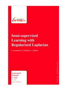
As an illustration, consider the bi-dimensional classification problem of Figure ... the goal of learning is to find a function which discriminates at best between red ...
Supervised learning with decision tree-based methods in computational and systems biology Pierre Geurts, Alexandre Irrthum, Louis Wehenkel Department of EE and CS & GIGA-Research, University of Liège, Belgium Abstract At the intersection between artificial intelligence and statistics, supervised learning provides algorithms to automatically build predictive models only from observations of a system. During the last twenty years, supervised learning has been a tool of choice to analyze the always increasing and complexifying data generated in the context of molecular biology, with successful applications in genome annotation, function prediction, or biomarker discovery. Among supervised learning methods, decision tree-based methods stand out as non parametric methods that have the unique feature of combining interpretability, efficiency, and, when used in ensembles of trees, excellent accuracy. The goal of this paper is to provide an accessible and comprehensive introduction to this class of methods. The first part of the paper is devoted to an intuitive but complete description of decision tree-based methods and a discussion of their strengths and limitations with respect to other supervised learning methods. The second part of the paper provides a survey of their applications in the context of computational and systems biology. The supplementary material provides information about various non-standard extensions of the decision tree-based approach to modeling, some practical guidelines for the choice of parameters and algorithm variants depending on the practical objectives of their application, pointers to freely accessible software packages, and a brief primer going through the different manipulations needed to use the tree-induction packages available in the R statistical tool.
Introduction Recent advances in experimental techniques have resulted in a dramatic increase of the amount and diversity of data being generated in the context of molecular biology. With tools such as microarrays, high-throughput sequencing, mass spectrometry, or advanced imaging techniques, measurements are possible at various scales and for more and more components of biological systems. The integration of all these data with available knowledge to better understand biological systems is at the heart of systems biology. The increase of complexity and dimensionality requires advanced computational approaches to store, organize, and analyze the data before they could be turned into novel biological knowledge. Among computational biology tools, machine learning naturally appears as one of the key components. In particular, supervised learning provides techniques to learn predictive models only from observations of a system and is thus particularly well suited to deal with the highly experimental nature of biological knowledge. Supervised learning has indeed been applied to a wide spectrum of problems in computational biology, ranging from genome annotations and structure prediction to the inference of networks of interactions between various kinds of biological entities, the prediction of protein functions, and the discovery of biomarkers and drugs. Among all supervised learning methods, this paper is devoted to a particular family of methods, called decision tree-based methods. Decision trees are among the most popular learning algorithms and they have been applied extensively in computational biology. The key ingredients of the success of these methods are their interpretability, that makes their model transparent and understandable to human experts, their flexibility, that makes them applicable to a wide range of problems, and their ease of use, that makes them accessible even to non-specialists. Combined with ensemble methods, they furthermore often provide state-of-the-art results in terms of predictive accuracy. Importantly in the context of high-throughput data sets, tree-based methods are also highly scalable from a computational point of view. The goal of this paper is to provide an accessible and comprehensive introduction to tree-based supervised learning methods and a survey of their applications in computational and systems biology. The 1
0.63
healthy
0.8
0.8
0.8
0.6
0.6
0.6 X2
Y sick healthy sick
1
X2
X2 0.35 0.94 0.08
1
X2
X1 0.19 0.44 0.63 ... 0.20
1
0.4
0.4
0.4
0.2
0.2
0.2
0
0 0
0.2
0.4
0.6
0.8
1
(a)
0 0
X1
(b)
0.2
0.4
0.6
0.8
1
0
0.2
0.4
0.6
X1
X1
(c)
(d)
0.8
1
Figure 1 An illustrative two-dimensional supervised learning problem. From left to right: (a) tabular learning sample, (b) scatter-plot of the learning sample together with the optimal classification boundary for this problem, (c) the classification boundary for a too simple model and (d) of a too complex one paper is structured as follows. We begin with a short introduction to supervised learning, with a discussion of the bias/variance tradeoff and of cross-validation methods. We then proceed with a detailed description of tree-based methods, starting with the main steps of standard decision tree induction, followed by a discussion of ensemble methods and tree-based attribute importance measures. We conclude this section with a discussion of the main strengths and limitations of these methods with respect to other supervised learning algorithms. The remainder of the paper is devoted to a survey of the main classes of applications of decision tree methods in the context of computational and systems biology. Supplementary material discusses several extensions of tree-based methods, gives some pointers towards freely available software packages implementing these methods, and provides a few practical guidelines on how to best exploit these methods, which are illustrated with an application in the R statistical language. The reading of this paper can be usefully complemented by a few other papers. An short intuitive review of decision trees can be found in Kingsford and Salzberg.1 Two more general introductions to machine learning in biology are given by Larrañaga et al 2 and by Tarca et al.3 Two other recent papers are dedicated to two other families of supervised learning methods and their applications in computational biology: support vector machines4 and artificial neural networks.5
Supervised learning In this section, we briefly introduce supervised learning. For more details, we refer the reader to general textbooks about supervised learning (and machine learning in general).6–8
Problem statement Machine learning denotes a broad class of computational methods which aim at extracting a model of a system from the sole observation (or the simulation) of this system in some situations. By the term model, we mean a set of exact or approximate relationships between the observed variables of the system. The goal of such models may be to predict the behavior of this system in some yet unobserved situations or to help understanding its already observed behavior. Supervised learning refers to the subset of machine learning methods which derive models in the form of input-output relationships. More precisely, the goal of supervised learning is to identify a mapping from some input variables to some output variables on the sole basis of a given sample of joint observations of the values of these variables. The (input or output) variables are often called attributes or features, while joint observations of their values are called objects and the given sample of objects used to infer a model is generally called the learning sample. As an illustration, consider the bi-dimensional classification problem of Figure 1 and assume that the goal of learning is to find a function which discriminates at best between red and green points. For example, each point of this space might represent a patient whose state is described by two input variables which are the result of two medical tests. Patients marked in red are those suffering from some disease while patients marked in green are the healthy ones. The goal could be to help a physician to predict the status of a new patient (the output) for which the test results are known (the inputs). In the real world, of course, each point of the learning sample is generally described by (many) more than
2
one or two input attributes and these attributes may have many other kinds of values than real numbers (discrete values, time series, images, sequences, for example). Also the output variables may represent more complex information than our binary decision variable. The above problem is the kind of problem targeted by supervised learning algorithms. Loosely speaking, a supervised learning algorithm receives a learning sample (like the one represented in Figure 1(a)) and returns an input-to-output function h (a hypothesis) which is chosen from a set of candidate models (its hypothesis space). Learning algorithms differ by the specific form of the hypotheses they consider (determined either by a parametric class of mathematical expressions or by a class of algorithmic procedures computing the outputs from the inputs), by their definition of the quality of hypotheses, and by the optimization strategy they use to find a high quality hypothesis in their hypothesis space. For example, a potential candidate function returned by a learning algorithm is the one given in Figure 1(b) in blue, represented by the decision boundary that it defines in the input space. Even though this function makes some mistakes on the learning sample, it seems that these mistakes are merely due to noise in the data (which may be due either to errors in measurements or to effects for which no input variables have been observed) and the function is thus a plausible explanation of the learning sample. As a matter of fact, for our toy problem, this particular input-output function turns out to be optimal in the sense that its predictions minimize the probability of mis-classification. An important criterion to assess learning algorithms, especially in the context of computational and systems biology, is the interpretability of the models that it infers from the data, i.e. the information that it may bring to a human expert about the studied input-output relationship. For example, in our medical application, it would be interesting to know if one of the two tests is not useful or not necessary to predict the disease status. Computational efficiency and scalability are also of great concern, especially for very large datasets, be it in the number of objects or the number of attributes. However, the main criterion used to assess learning algorithms is their prediction accuracy, i.e. the way the model they produce generalizes to unseen data (i.e. data that were not observed in the learning sample).
Bias-variance tradeoff To explain why supervised learning of models with good predictive accuracy is not trivial, it is necessary to understand the bias/variance tradeoff in this context. To give some intuition about this tradeoff, let us first assume that we want to separate the two classes in Figure 1 with a linear decision boundary. Figure 1(c) shows one such model illustrating the fact that with linear models it is impossible to discriminate well enough the two classes of our toy problem. The family of linear models is not well suited to solve our task because the best linear model is too far from an optimal decision boundary like the one represented at Figure 1(b), whatever the amount of data used to infer it. This source of error is called bias. Let us assume now that we use a much larger family of hypotheses among which there exist one or several which realize a perfect separation between classes in our learning sample. Then, by using this hypothesis space, the learning algorithm might produce a decision boundary like the one shown on Figure 1(d). This time, the classification boundary perfectly separates all learning objects of different classes. Like the linear model however, this model is still not appropriate. This time, the model is too complex and hence it learns “too much” information from our data. In this case, we say that the learning algorithm overfits the data. If we would use another learning sample for the same problem (e.g. by repeating the experiment on another group of patients), then it would be very likely that the model found by the same learning algorithm would be very different from the one of Figure 1(d). In this case, we say that the learning algorithm suffers from variance, because the hypothesis that it returns for a given problem is very much dependent on the particular learning sample that is provided. When it comes to apply the hypothesis inferred by supervised learning on new objects, both bias and variance are sources of error and hence they should ideally both be minimal. Moreover, as they react in an opposite direction to variations of the complexity of the hypothesis space, there is a tradeoff between their effects which must be taken into account. Because of its central role in supervised learning, this tradeoff has received a lot of attention in the design of supervised learning algorithms. The main approach to handle it is to adapt the complexity of the hypothesis space to the problem under consideration (during learning), e.g. by using cross-validation to select meta-parameters controlling the complexity of the hypothesis space.
3
Assessment by cross-validation The evaluation of the predictive accuracy of a model is crucial in supervised learning, first in order to predict its future performance on new data but also in order to provide the learning algorithm with a criterion to choose a model in its hypothesis space. Evaluation requires the choice of an estimation procedure and of a performance measure. Usually the performance of the model as estimated on the learning sample, called resubstitution estimate, is a very optimistic estimate of the true quality of the model. A more reliable estimate would be obtained from a sample independent of the data sample used during the learning stage. For example, a hold-out estimate is obtained by partitioning the learning sample ls into two disjoint subsets, the validation sample vs and the learning sample ls without the objects in vs, denoted ls\vs. A model is learned from ls\vs and its performance is assessed on vs. A common practice is to save one third of the data for the validation. However, when the learning sample is very small, subdividing further the data will yield an unreliable estimate. In these cases, cross-validation provides a way to make a better use of the available sample. In S k-foldScross-validation, we divide the learning sample into k disjoint subsets S of the same size, ls = ls1 ls2 . . . lsk . A model is then inferred by the learning algorithm from each sample ls\lsi, i = 1, . . . , k and its performance is determined on the held out sample lsi . The final performance is computed as the average performance over all these models. Notice that when k is equal to the number of objects in the learning sample, this method is called leave-one-out. Typically, smaller values of k (say, between 10 and 20) are however preferred for computational reasons. Notice that when cross-validation is used to make a selection between several models (e.g. corresponding to different values of the meta-parameters of a learning algorithm or produced by different learning algorithms), then an additional external run of cross-validation is necessary to provide also a reliable estimate of the finally chosen model.9 Evaluation also raises the question of the choice of a performance measure. This choice usually depends on the application. In the context of classification, i.e. when the output variable is discrete, the most common measure is the error rate of the model (i.e. the probability of making a wrong prediction as estimated for example by the proportion of wrong predictions on the validation sample). The main drawback of this measure is that it is sensitive to the proportion of objects of different classes in the validation sample and that it does not convey information about the kind of errors. In the context of binary classification, it is therefore usually complemented by other measures such as sensitivity (the proportion of objects in the class of interest that are well classified) or specificity (the proportion of objects in the other class that are well classified). Moreover, since most classifiers inferred by supervised learning actually produce a confidence score (e.g., in the form of a class probability estimate), in the case of binary classification problems, one may use different thresholds on this score to achieve different compromises between sensitivity and specificity. To evaluate a model independently of the chosen threshold, one can use a ROC curve,10 that plots true positive rate (sensitivity) versus false positive rate (1-specificity) for different values of this threshold. The quality of a ROC curve is evaluated by the area under this curve (AUC), as we will illustrate below.
Decision tree induction Decision tree induction11, 12 is currently one of the most interesting supervised learning algorithms. The paternity of tree-based learning methods is often attributed to Hunt with his Concept Learning System.13 Later on, the method was formalized, extended, and popularized in the field of statistics by the famous book of Breiman, Friedman, Olsen, and Stone on Classification And Regression Trees (CART11 ). During the same period, Quinlan also contributed to the dissemination of this approach in the field of artificial intelligence with his ID314 and C4.512 algorithms. Let us notice that decision tree induction, originally designed to solve classification problems, have been extended to handle more complex output spaces (e.g. single- or multi-dimensional regression). For the sake of simplicity, we will focus on the case of classification trees and describe in this context the main ideas behind this methodology. We will then discuss its main strengths and weaknesses with respect to other supervised learning methods. For advanced readers, the supplementary material elaborates on the extensions of the basic decision tree framework, in particular to regression.
4
X2