Research and applications
Supervised machine learning and active learning in classification of radiology reports Dung H M Nguyen, Jon D Patrick ▸ Additional material is published online only. To view please visit the journal online (http://dx.doi.org/10.1136/ amiajnl-2013-002516). School of Information Technologies, University of Sydney, Sydney, New South Wales, Australia Correspondence to Dr Dung H M Nguyen, School of Information Technologies, University of Sydney, 1 Cleveland St, Sydney, NSW 2006, Australia;
[email protected] Received 18 November 2013 Revised 7 April 2014 Accepted 29 April 2014 Published Online First 22 May 2014
ABSTRACT Objective This paper presents an automated system for classifying the results of imaging examinations (CT, MRI, positron emission tomography) into reportable and non-reportable cancer cases. This system is part of an industrial-strength processing pipeline built to extract content from radiology reports for use in the Victorian Cancer Registry. Materials and methods In addition to traditional supervised learning methods such as conditional random fields and support vector machines, active learning (AL) approaches were investigated to optimize training production and further improve classification performance. The project involved two pilot sites in Victoria, Australia (Lake Imaging (Ballarat) and Peter MacCallum Cancer Centre (Melbourne)) and, in collaboration with the NSW Central Registry, one pilot site at Westmead Hospital (Sydney). Results The reportability classifier performance achieved 98.25% sensitivity and 96.14% specificity on the cancer registry’s held-out test set. Up to 92% of training data needed for supervised machine learning can be saved by AL. Discussion AL is a promising method for optimizing the supervised training production used in classification of radiology reports. When an AL strategy is applied during the data selection process, the cost of manual classification can be reduced significantly. Conclusions The most important practical application of the reportability classifier is that it can dramatically reduce human effort in identifying relevant reports from the large imaging pool for further investigation of cancer. The classifier is built on a large real-world dataset and can achieve high performance in filtering relevant reports to support cancer registries.
OBJECTIVE
To cite: Nguyen DHM, Patrick JD. J Am Med Inform Assoc 2014;21:893–901.
The aim of this study was to develop an automated system for classification of radiology reports, which uses active learning (AL) solutions to build optimal supervised machine learning models. The optimal model is the one that can generate the best performance with minimal cost in manual classification. The classification data used in this research were contributed by experienced coders, and the authors of the reports were all experienced radiologists. The study focused on identifying reportable cases to be provided to the registry. A parallel study checking the coincidence of radiology reports with pathology reports and hospital records will be prepared by the registry. This research used the special strategy of producing a reportability classifier that separates cancer and non-cancer reports by using a deliberate bias to ensure that virtually all cancer reports are
Nguyen DHM, et al. J Am Med Inform Assoc 2014;21:893–901. doi:10.1136/amiajnl-2013-002516
recognized. This has the consequence of producing high sensitivity while maintaining reasonable specificity. Ideally, the cancer registry does not want to miss any cancer cases; however, it accepts sensitivity better than 98% and specificity higher than 96%.
BACKGROUND AND SIGNIFICANCE This is a research project to determine the effectiveness of making the first identification of cancer rather than post a pathology report. Radiology reports have a number of advantages over pathology reports in this task: they can provide staging at the initial diagnosis, where a pathology sample is not taken; they provide a diagnosis when a sample will not be taken; and they present the progress of the disease over time. At cancer registries, a large number of radiology reports need to be manually reviewed each year to identify the cancer cases. This process is very timeconsuming because most reports in the whole pool are not related to cancer. On average, coders have to read nine reports to identify only one case that is applicable for further investigation. This becomes a significant workload when each registry can receive more than 100 000 records per year. The distribution between cancer and non-cancer classes also poses an imbalanced data problem for selection of the training data used for supervised machine learning. Machine learning systems have demonstrated high accuracy in automatic classification of radiology reports. Thomas et al1 used Boolean logic built from 512 consecutive ankle radiography reports to create a text search algorithm and then applied it to a different set of 750 radiology reports to obtain a sensitivity of 87.8% and specificity of 91.3%. The LEXIMER automated engine classified 1059 unstructured reports of radiology examinations based on the presence of important findings and suggested further actions with 94.9% sensitivity and 97.7% specificity.2 In other research specializing in lung cancer reports, McCowan and Moore3 used support vector machine (SVM) learning techniques to investigate the classification of cancer stages. This system achieved an accuracy of 74% for tumor (T) staging and 87% for node (N) staging on the complete 179-case trial dataset. Cheng et al4 first assessed whether the text contained sufficient information for a classification process and then determined tumor status and progression using SVM models that reached 80.6% sensitivity and 91.6% specificity. However, the sizes of the corpora used in previous research were relatively small compared with the number of reports processed by a registry each year. The 893
Research and applications performance of a machine learning system is usually decreased with a small dataset because a small number of samples will cause a broad CI around performance estimates. Furthermore, there is no investigation of AL approaches reported in related work on classification of radiology reports. AL is a subfield of machine learning where the learner is allowed to query the most informative instances to retrain the model instead of making a random selection. On the basis of this approach, with the same number of sample selections, the performance of active learners exceeds that of random learners in most cases.5 The AL approach requires significantly fewer manually classified reports while maintaining comparable performance to traditional supervised learning with all training data—or even bettering it. AL can also help to reduce the problem of an imbalanced dataset by not querying the redundant samples from the dominated class.6 Many AL algorithms have been introduced in the literature. The four algorithms investigated in this research are Simple, Self-Confident (Self-Conf ), Kernel Farthest-First (KFF), and Balanced Exploration and Exploitation (Balance-EE).7–13 These algorithms appear to be among the best performers based on empirical studies.7–8 Furthermore, they are reasonably well motivated and achieved high performance on real-world data. In the clinical domain, AL approaches were recently investigated by Chen et al14 15 with the applications of word sense disambiguation and high-throughput phenotyping algorithms. For clinical text classification, Figueroa et al16 concluded that appropriate AL algorithms can yield comparable performance to that of random learning with significantly smaller training sets. Furthermore, the AL-inspired method has been used to find optimal training sets for Bayesian prediction of medical subject headings, which produced ∼200% improvement over use of previous training sets.17
MATERIALS AND METHODS Data description The cancer cases covered in this study included all reports provided in a year’s data collection by the imaging service. The process of creating the classifiers relied on using a manually trained corpus drawn from each site. Initially, a sample of 16 472 reports was drawn from Lake Imaging and assigned to cancer (4784 reports) or non-cancer (11 688 reports) classes by the cancer registry and then incrementally delivered to our system. The distribution of the cancer types was: digestive systems (21.85%), lymphoid (17.87%), lung (15.84%), genitourinary (10.72%), breast (8.30%), head and neck (5.24%), skin (5.05%), central nervous system (3.44%), gynecologic (4.40%), unknown/not specified (7.04%), and other/specified (including ophthalmic sites) (0.23%).
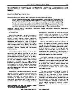
System architecture Figure 1 presents the system architecture for classification of radiology reports. The processing pipeline comprises three phases: preprocessing, training, and testing. The preprocessing phase is responsible for proofreading the corpus and preparing it for annotation and classification tasks. First, the texts are split into tokens and clinical patterns by a ring-fencing tokenizer.18 Then, the tokens are validated by the lexical verification process using our accumulated lexicon resource. This resource contains categorization of spelling errors, abbreviations and acronyms in the clinical domain. The training phase includes processes for constructing entity taggers and report classifiers. The automated entity tagger is used to improve the performance of the classification process 894
and identify the components needed to complete extraction of cancer staging and recurrence. Initially, free-text cancer reports are annotated for examples of the entities to be identified, and then algorithms are developed that use the examples to compute a conditional random fields (CRF) tagger model.19 The model is evaluated and the algorithm revised in a feedback process to produce a more accurate result. The interactive annotation process is continued over a series of experiments until an optimal model is identified. This not only reduces the workload and annotation time per report but also reduces the error rate and inconsistencies of human annotation generated by different levels of expertise. The classification training process is similar to constructing entity taggers except that (i) the training sets contain both cancer and non-cancer reports, (ii) tagging models are used to generate features for training SVM classifiers,20 and (iii) the AL approach is used to select the most informative reports to add to the current training set when new reports or new corpora are available. In the test phase, the test set is first annotated by the CRF models to prepare features for SVM classification. Finally, the rule-based postprocessing system is applied to improve the sensitivity of the classifier. In general, the rules will investigate all the reports that have been recognized by the classifier as nonreportable to capture as many as possible missed classified reportables.
Annotation schema for cancer-related information To support the classification process, the training reports are tagged to identify structure and cancer-related information based on a well-designed annotation schema (see online supplementary material). The tag set in this schema should contain enough detail to distinguish between cancer and non-cancer cases as well as complete a staging report. Instead of using a general medical terminology such as the Unified Medical Language System (UMLS) or SNOMED-CT (Systematized Nomenclature of Medicine-Clinical Terms) (or their subsets) to identify clinical entities in the text, we have designed our own tag set, which is much more relevant to the cancer information extraction task.21 22 Our designed tag sets are well controlled and do not contain superfluous information, which can mislead the classification process. The tags can be divided into five subsets. 1. Descriptor subset: morphology, topography, cytomorphology and modality type tags. ▸ Morphology describes the object of interest’s shape, structure, and behavior (behavior, structure, size). ▸ Topography locates the object of interest spatially (laterally, location, site). ▸ Cytomorphology identifies cell level morphology (cell growth pattern, cell type, tissue type). 2. Entity subset: objects of interest within a report. They are usually the subject of the report, which is cancer in this case. ▸ A disorder of fluid, gas or other noted by the radiologist or referring doctor (disorder). ▸ A non-cancerous anatomic or metabolic abnormality being described during the report (generic lesion). ▸ The primary tumor being described by the radiologist, cancerous ( primary). ▸ Recurrence of a pre-existing cancer (recurrence). ▸ Spread of cancer from one part of the body to another (metastases). ▸ A rounded mass of lymphatic tissue that is surrounded by a capsule of connective tissue (node). This tag picks up the entity itself and this entity will have certain values attached—for example, site, size, shape.
Nguyen DHM, et al. J Am Med Inform Assoc 2014;21:893–901. doi:10.1136/amiajnl-2013-002516
Research and applications
Figure 1 System architecture. CRF, conditional random fields; SVM, support vector machine.
3. Linguistic subset: includes lexical polarity, normality and modifier tags. Linguistic tags are not directly related to cancer content, but they are crucial for the confirmation of reportability. ▸ Lexical polarity negative (LPN) and lexical polarity positive to define existence or non-existence of phrases at a lexical level. ▸ Normality negative and normality positive define normality or abnormality. ▸ Modality, mood and comment adjuncts, numerative and temporality are used as modifiers. 4. Radiologist’s coding subset: includes cancer stage, TNM (tumor-nodal-metastases) values which are recorded directly in the text. ▸ Staging describes the extent or severity of the cancer (anatomic stage). Knowing the stage of a disease helps treatment planning and prognosis. This will be clinical or pathologic. ▸ Extent or spread of the tumor (T value). ▸ Spread of cancer cells to nearby (regional) lymph nodes (N value). ▸ Distant (to other parts of the body) metastasis has occurred (M value). 5. Structure subset: includes heading tags. The structure tags are not directly related to the cancer content but support the use of context as features in the classification process. These headings are also used to structure the report body when populating the output in an XML format.
▸ Headings that pertain to the history of the patient (clinical history heading). ▸ Headings that pertain to the conclusive summary generally present at the end of the report (conclusions heading). ▸ Headings that create a boundary for the findings (findings heading). ▸ Miscellaneous subheadings that do not fall under the aforementioned structural heading tags, especially when there are multiple objects of interest that occur within a report or it is a combined report (subheading). A detailed and well-designed tagging system can contribute significantly to the classification and extraction results. For example, the sentence ‘There is no convincing metastatic bone lesion’ in the conclusion will be tagged as: There is |{z} no convincing metastatic bone lesion |fflfflfflfflfflfflffl{zfflfflfflfflfflfflffl} |fflfflfflfflfflffl{zfflfflfflfflfflffl} |ffl{zffl} |fflffl{zfflffl} LPN
Modality
Metastases
Site
Lesion
The occurrence of popular cancer terms in one sentence in the conclusion section is not enough to conclude that the cancer is reportable. The complete investigation has to consider whether the cancer term is negated or modalised on the basis of linguistic tags such as LPN and modality in the classification process. The performance of the tagging system is important to the success of both machine learning and rule-based methods. More than 3000 cancer reports were annotated with ∼500 000 tag instances. The overall F-score was ∼97.5% for the self-
Nguyen DHM, et al. J Am Med Inform Assoc 2014;21:893–901. doi:10.1136/amiajnl-2013-002516
895
Research and applications Table 1
Fivefold cross-validation tagging performance
Subset
True positives
False positives
False negatives
Precision (%)
Recall (%)
F-score (%)
Descriptor Entity Radiologist Linguistic Structure Overall
230 615 71 340 1417 141 257 20 370 464 999
17 980 6214 114 8464 204 32 976
16 682 7640 182 8948 391 33 843
92.8 92.0 92.6 94.4 99.0 93.4
93.3 90.3 88.6 94.0 98.1 93.2
93.0 91.2 90.5 94.2 98.6 93.3
validation process, which means using all training data to train the model and test on the same data. This self-test result indicates the level of annotation consistency in the corpus. The common approach to evaluating the performance of the model is cross-validation. The overall F-score for fivefold crossvalidation of the Named-Entity Recognizer (NER) is ∼93% (table 1). This means the training data are randomly divided into five folds, and each fold is retained as validation data and the remaining four folds are used as training data. The F-score is then computed as the average performance of five testing folds. The CRF++ tool is used in our NER experiments, and the best performance was obtained from the following feature sets.23 ▸ Bag-of-words (BOW) in lower case with a five-word context window. ▸ Proofreading features: corrections and expansions, when used as features, will support the model in learning correct forms of misspelled words (‘medicla’ and ‘medcial’ refer to the same word ‘medical’) and variations of abbreviations (‘amnt’ and ‘amt’ are both ‘amount’), and multiple acronyms of the same term (‘ABG’ and ‘ABGs’ are both ‘arterial blood gases’). ▸ Ring fencing: the basic patterns (eg, date, time, number) and standard patterns (eg, blood pressure, heart rate, cancer stage) are used as features to indicate whether a token belongs to any kind of measures and scores.
Feature generation for SVMs For a large-scale classification problem with many thousands of instances and features such as in the reportability classification task, a linear kernel is usually a promising learning technique.24 Experiments were therefore performed with optimized linear kernel (Liblinear) as the base classifier rather than SVMs with nonlinear kernels. Liblinear is an open source library for large-scale linear classification with ease of solver and parameter selection.25 The best performance was obtained from five feature sets. ▸ BOW binary term weight: for linear and large-scale classification problems such as in radiology reports. The binary term weight with a small penalty parameter C can have similar accuracy to the best performance of frequency term weight with normalized vectors. The feature value of the binary term weight is 0 or 1 corresponding to the existence of that feature in the text. ▸ Bag-of-tags (BOT): a binary term weight is assigned to tokens tagged by the computational tagger. The feature value is 1 if a tag is assigned by the tagger. ▸ Gazetteer feature: checks whether a term belongs to a specialized cancer term gazetteer created by the linguists. ▸ Context feature: adds features to indicate whether a word belongs to a specific context (eg, clinical indication, conclusion). The heading tags from annotation results are identifiers 896
for the start and end of each section, where the start of the next section is the end of the previous section. ▸ Negation and modality feature: the occurrence of negation and modality tags can identify whether a phrase is modalised or negated.
Active learning This section briefly introduces the key ideas behind the four AL strategies (Simple, Self-Conf, KFF and Balanced-EE) investigated in the present research. The Simple algorithm is based on the kernel machines and was independently proposed by three different research groups.9–11 The name Simple (simple margin) came from Tong et al10 and used uncertainty estimation as its selection strategy. In SVM kernel space, the highest uncertain instance, which is defined as the most informative instance, is the one that lies closest to the decision hyperplane. For each unlabeled instance x, the shortest distance between the feature vector, ɸ(x), and the hyperplane, wi, in the feature space is easily computed by | wi.ɸ (x)|. Hence, the querying function of Simple uses the current classifier to choose an unlabeled instance which is closest to the decision boundary. Other variations of Simple margin include MaxMin margin and Ratio margin, which consider the sizes of version space during the selection process. The Self-Conf algorithm chooses the next example to be labeled so that, when it is added to the training data, the future generalization error probability is minimized. Since true future error rates are unknown, the learner attempts to estimate them using a ‘self-confidence’ heuristic, which uses its current classifier for probability measurements. The future error rate is estimated by a log-loss function, which uses the entropy of the posterior class distribution on a sample of the unlabeled instances. Each instance from the unseen pool is examined by adding it to the training set with a sample of its possible labels and estimating the resulting future error rate; the instance with the smallest expected log is then chosen. However, in each selection round, the expected log-loss is recalculated for all instances in the unseen pool based on their possible labels, and then the model is retrained. As a consequence, this algorithm is exceedingly inefficient. Many optimization and approximation approaches were proposed by Roy and McCallum to achieve a practical running time.12 The Self-Conf algorithm implemented in this paper only uses random subsampling: on each query, the expected error is estimated for a random subset of unseen data.7 The size of this subset can be adjusted during the selection process. The KFF algorithm uses a simple AL heuristic based on the ‘farthest-first’ traversal sequence in kernel space.13 In this algorithm, the most informative instance is the farthest instance in the unseen pool from the current training set, where the distance from a point to a set is defined as the Euclidean distance
Nguyen DHM, et al. J Am Med Inform Assoc 2014;21:893–901. doi:10.1136/amiajnl-2013-002516
Research and applications Table 2 Distribution of tags in sections of the radiology reports
Descriptor Entity Linguistic Radiologist’s coding
Clinical history
Conclusions
Findings
Subheading
23 637 (9.51%) 8785 (11.33%) 111 (7.25%) 31 083 (20.76%)
33 260 15 525 238 100 130
66 080 16 504 399 791
125 618 36 740 783 17 717
to the closest point in the set. The assumption behind the KFF heuristic is that the farthest instance is considered to be the most dissimilar to the current training data and needs to be learned first. The advantage of KFF over Simple and Self-Conf algorithms is that it does not use the model to evaluate the unseen pool during the querying process. Hence, there is no need to retrain the model after each AL trial, and it can be applied to any learning algorithms. The Simple active learner is good at ‘exploitation’ by selecting the examples near the boundary, but it does not carry out ‘exploration’ by searching for large regions in the instance space that it might incorrectly predict. Osugi et al8 introduced the Balance-EE method, which is based on a combination of Simple and KFF, to address the problem of balancing between exploitation of labeling instances that are near the current decision boundary (Simple) and exploration by searching for instances that are far from the already labeled points (KFF).13 At each trial, Balance-EE randomly decides whether exploration (Simple) or exploitation (KFF) will be used. If the choice is exploration (Simple), the algorithm evaluates the efficiency of the exploration to adjust its probability of exploring again. We then compared the performances of random sampling and the four active sampling algorithms presented above using the radiology reports dataset. The training set comprised 14 824 examples (including 4325 reportables), which is nine times larger than the test set with 1647 examples (including 459 reportables). The training and test sets were randomly selected from the radiology corpus. The final AL approach used to build the classifier is Simple with uncertainty estimation. From the results of the experiments with the four different AL algorithms, it was the most efficient algorithm in terms of complexity and performance. Retraining and evaluating the model after single selection is extremely inefficient, especially when the training size increases. Hence, to speed up the process, the queries were executed in batches of 10 in each learning trial, and then the classifier was retrained. The AL algorithms stopped querying new instances when the following criteria were met: the F-score exceed 95% and there was no significant increase from the active learners. After 100 rounds of selection, the total number of selected examples was 1002 for each sampling method, where the initial training set included one positive and one negative class which were randomly selected.
(13.38%) (20.02%) (15.55%) (66.88%)
(25.58%) (21.28%) (26.06%) (0.53%)
(50.53%) (47.37%) (51.14%) (11.83%)
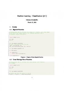
large dataset with thousands of reports, as they will usually provide high precision but low recall. The basic advantage of supervised machine learning is that the concept characteristics and classification rules can be automatically learnt through training examples. Hence, it is preferable to have a large dataset. In general, the main purpose of the rules in this research is to capture as many cancer reports as possible. Thus, these rules were only applied for files that had been classified as nonreportable by the machine learner. The rules were designed by linguists on the basis of a combination of gazetteers and computational tags. The gazetteers are lists of cancer and treatment terms that are commonly found in reportable cases that distinguish them from the non-reportable cases. The computational tags play an important role in supporting the rules. First, the rules are only operated within specific sections such as the conclusion or clinical findings, where these section headings are well captured by the tagging model. The distribution of tag classes within different sections of the radiology reports is shown in table 2. Second, the existences of tag types such as recurrence, LPN and modality within a sentence are used by the rules. Figure 2 illustrates one of five decision rules applied for each cancer term that is found in the conclusions section. The postprocessing system contains a list of rules that are applied in sequence when a previous rule has failed to identify the report as a reportable cancer.
Rule-based postprocessing system At the end of the AL process, 1000 reports were selected by the Simple method to build the SVM classifier. To meet the special research requirement of high sensitivity, the active machine learner was then supported by the rule-based postprocessing system. Rules are usually designed by experts to capture specific patterns or keywords in the text by looking at several examples. They are limited by the number of examples the experts can examine. Hence, it is very difficult to use rules to describe a
Figure 2 Example of a postprocessing rule. LPN, Lexical polarity negative.
Nguyen DHM, et al. J Am Med Inform Assoc 2014;21:893–901. doi:10.1136/amiajnl-2013-002516
897
Research and applications
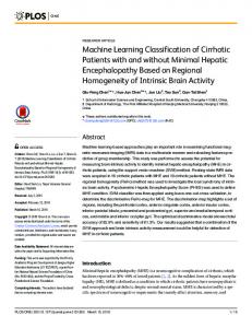
Figure 3 Evaluation of active and random sampling on test data. AL, active learning; Balance, Balanced Exploration and Exploitation algorithm; KFF, Kernel Farthest-First algorithm; Self, Self-Confident algorithm.
RESULTS Active learning Figure 3 shows the accuracy of the four AL algorithms and random sampling in classifying the radiology reports. Random sampling gave a consistent performance of ∼72.13% throughout the learning process; this accuracy is equal to the rate of nonreportable instances in the test set (1188/1647). Except for the last few cycles which can only capture one or two positive instances, the random classifier predicted every instance in the test set as non-reportable. This is because the number of nonreportables in the training set is 2.6 times greater than the number of reportables, so they exceeded the reportable instances in the random selection. The worst performance can be seen with the KFF algorithm, with 27.87% over time; this accuracy is equal to the rate of reportables in the test set (459/ 1647). Different from the random sampling, the KFF algorithm mostly selected the positive class (766 positives out of 1002 selected examples). Hence, the KFF classifier categorized all instances in the test set as reportable. The three other AL algorithms show comparable results, with over 94.5% accuracy at the peak points. Balance-EE is a combination of Simple and KFF with a choice of algorithm in each trial. In this experiment, KFF was selected by Balance-EE for the first six trials for 60 examples, and then Simple was applied for the subsequent instances. As a result, except for several ‘drop points,’ Balance-EE had a similar learning curve to Simple 898
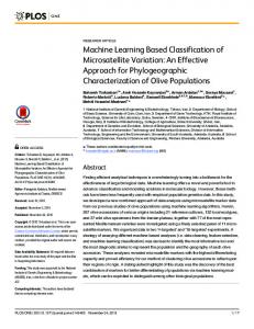
because most examples were selected using the ‘exploitation’ (Simple) strategy. The Self-Conf algorithm showed consistently higher accuracy than Simple and Balance-EE for the initial AL queries, and it quickly reached the top performance with only 60% queries used. Figure 4 presents the performances of the four AL algorithms and random sampling for identification of reportables. In this experiment, the random sampling method could not identify any reportables in the test set until the number of queries reached 80%; from then on, its F-scores were still relatively low, 90.5%. However, the gaps from ‘drop points’ to the closest neighbors are more significant than the analysis on two classes. The full learning curves for Simple active sampling and random sampling with a batch size of 100 reports per round for 145 rounds are presented in figure 5. The batch size was increased from 10 to 100 to speed up the process in order to generate an overview of the comprehensive learning curves. However, the performance of the active learner with the same training size was reduced because the model was updated 10 times less frequently. Figure 5 shows that the performance of the random sampler increased only when it had 3000 reports.
Nguyen DHM, et al. J Am Med Inform Assoc 2014;21:893–901. doi:10.1136/amiajnl-2013-002516
Research and applications
Figure 4 Evaluation of active and random sampling on test data for identifying reportable cases. AL, active learning; Balance, Balanced Exploration and Exploitation algorithm; KFF, Kernel Farthest-First algorithm; Self, Self-Confident algorithm. At that point, the Simple active learner had already reached its top performance, which was >23% higher than the random learner. There was not much difference in the performances of the two methods when 10 000 reports were selected. A known problem with many AL algorithms, especially in the early steps of learning, is that they are prone to generate a biased training set rather than be representative of the true underlying data distribution.26 As can be seen in figure 5, there are a few points where the performance of the active learner dropped dramatically —for example, the performance fell below 80% when 1600 samples were used. This is due to limitations in the initial model that will perform AL. Many algorithms just randomly select a few instances to train the first model, which is usually not a good starting point for the real data distribution.
Evaluation on the held-out test set The evaluation of the reportability classifier presented here was executed independently at the Cancer Registry. They used sensitivity and specificity as evaluation metrics, while precision, recall, and F1-score were calculated in our experiments. For the binary classification problem, ‘sensitivity’ is equal to ‘recall’ of the positive class (reportable), and ‘specificity’ is the ‘recall’ of the negative class (non-reportable). The Registry maintains the held-out test set to evaluate the system independently until the required sensitivity and specificity are achieved. None of the
held-out test set was used for any part of the system development —for example, they were not used to build the gazetteers or the rule-based approaches. This held-out test set comprised 400 reportables and 2100 non-reportables, which is a similar distribution to the released data. The approved version achieved a sensitivity of 98.25% and specificity of 96.14%. This version is implemented on the basis of the two machine learning methods (CRFs and SVMs) and a rule-based postprocessing system (table 2). The special cancer gazetteers collected by linguists who are experienced in interpreting the reports are used to support both the machine learning and rule approaches.
DISCUSSION From these analyses, the Simple algorithm was chosen as the AL strategy for generating the priority list for manual reportability classification of radiology reports. As seen in figure 2, the Simple method had comparable results to Self-Conf and Balanced-EE, but implementation was simpler and more efficient. For 100 trials, Balanced-EE was slightly slower than Simple, while Self-Conf was five times slower than Simple. From table 3, although adding rules significantly increased sensitivity without affecting specificity, it is only useful in combination with machine learning approaches, since a rule-based classifier alone never reached an F-score of 80%. With this performance for evaluation on the held-out test set, the main objective of the automatic classification system was satisfied,
Nguyen DHM, et al. J Am Med Inform Assoc 2014;21:893–901. doi:10.1136/amiajnl-2013-002516
899
Research and applications
Figure 5 Full learning curves for Simple active learning and random learning with a batch size of 100. AL, active learning.
with sensitivity higher than 98% while maintaining a specificity of no lower than 96%. When the AL strategy was applied during the data selection process, the cost of manual classification was reduced significantly. The overall F-score of the active classifier built on