Supervised Strategies For Cracks Detection In Images Of ... - eurasip

16th European Signal Processing Conference (EUSIPCO 2008), Lausanne, Switzerland, August 25-29, 2008, copyright by EURASIP

SUPERVISED STRATEGIES FOR CRACKS DETECTION IN IMAGES OF ROAD PAVEMENT FLEXIBLE SURFACES Henrique Oliveira1,2, Paulo Lobato Correia1 1

Instituto de Telecomunicações – Instituto Superior Técnico, Universidade Técnica de Lisboa Av. Rovisco Pais, 1, 1049-001 Lisboa, Portugal 2 Escola Superior de Tecnologia e Gestão – Instituto Politécnico de Beja Rua Afonso III, 1, 7800-050 Beja, Portugal [email protected], [email protected] ABSTRACT

The detection of cracks and other degradations in road pavement surfaces is traditionally done by experts using visual inspection, while driving along the surveyed road. An automatic cracks detection system based on road pavement images, as proposed here, can speed up the process and reduce results’ subjectivity. The paper confronts six supervised classification strategies, three parametric and three non-parametric. The analysis is done on data resulting from dividing the image into a set of non-overlapping windows. Dealing with supervised classification strategies, a technique for automatic selection of training images from an image database is proposed as the initial step, after which a human expert should select the image windows containing cracks. The selected classification strategies work with a 2D feature space. Classifiers are evaluated using a set of well-know metrics, indicating that a better performance can be achieved using parametric classification strategies. 1.

INTRODUCTION

The main objectives of using automatic systems for cracks detection in road pavement flexible surfaces are to reduce subjectivity in traditional human inspection and to speed up the surveys, resulting in less dangerous situations, especially while driving in high speed roads like highways [1]. A description of commercial systems used since the 1970’s is presented in [2], typically including complex and very expensive hardware [3], in opposition to the low cost solution presented in this paper. Digital images are typically the most important source of information for qualitative and quantitative evaluation of crack distresses. Neural networks, Markov random fields and edge detectors have been considered for the development of automatic crack distress detection systems [4]. This paper considers supervised classification strategies, confronting six pattern classifiers (three parametric and three non-parametric) for automatic cracks detection in images of road pavement flexible surfaces. An image database has been created by surveying some Portuguese roads. Disjoint subsets of these images are used for training and testing the classifiers. All the analysis is done on data resulting from dividing The authors acknowledge the support from Fundação para a Ciência e Tecnologia (FCT).

the images into a set of non-overlapping windows. The acquired images are pre-processed using normalization techniques to reduce the influence of noise and some irrelevant properties of the road upper layer aggregates. Since this paper deals with supervised classification strategies, the initial step is the selection of images for classifier training. These images are presented to the human operator for selection of image windows containing cracks. The proposed classification strategies work with a, previously normalized, 2D feature space. For each of the considered classifiers a decision boundary is computed, during the training stage. The classifiers performance is evaluated using Errorrate, Recall, Precision and performance metrics, computed for all the images of the test set for which a ground truth is available, from a manual classification previously performed. Section 2 discusses image acquisition, the automatic selection of a set of training images, image normalization and feature extraction and normalization. Section 3 describes the classifiers used and the associated parameters. Section 4 presents experimental results and their analysis. Conclusions and some hints for future work are addressed in Section 5. 2.

CRACK DETECTION SUPERVISED STRATEGIES

The supervised cracks detection system proposed is implemented in two steps: training and testing. These main steps follow a set of normalization procedures to ensure a correct operation of the classifiers. Training is a learning phase for the classifiers, in which they learn from samples manually labeled by a human operator, indicating for each training image if a window contains cracks. During the test phase, images are classified as containing pavement cracks, or not. Again, the analysis is performed at a window level. A proposal for an automatic selection of the images to be used for training is presented, based on a pre-analysis of the available images. For an appropriate training of the classifiers the selected training images should contain cracks. The diagram presented in Figure 1 shows the global architecture for the proposed supervised classification strategies. 2.1 Image acquisition The image database considered in this paper is composed by grayscale images acquired during a pavement surface visual survey over a Portuguese road. A digital camera was placed with its optical axis perpendicular to the road surface, at


different vertical distances (between 1.0 m and 1.5 m from the pavement surface), providing images with different spatial resolutions. Images with different sizes are considered (from 2048×1536 to 1858×1384), as they only contain areas belonging to the road pavement surface. Image

database

Selection of training images Image normalization

[

Feature extraction and normalization Training Parametric learning Decision

Features (test set)

Non-parametric learning

(

(

Evaluation

Figure 1 – System architecture. 2.2 Selection of training images Training images should contain road pavement cracks, to allow a correct learning stage for the classifiers. Here, an automatic training set selection procedure is proposed. A human operator should then (manually) identify the regions that contain cracks. To speed up the lengthy and costly manual procedure, the human operator does not perform a pixel based annotation of the cracks present in images. Rather, he operates with a set of non-overlapping image windows, of size 75×75 pixels. This dimension was empirically chosen, providing a good compromise between complexity and accuracy. The selection of training images recurs to a preliminary classification phase, exploiting the knowledge that windows with cracks are supposed to have lower mean intensity values, when compared to windows without cracks. A matrix of window mean intensity values is computed for each image. Given the image and window sizes considered, the resulting matrices can have dimensions between 27×20 and 24×18. The algorithm for preliminary detection of cracks starts with separate vertical and horizontal scans of the mean matrices, supported by a logical decision (ld). During the vertical scan, each column, j, of the matrix is analyzed (with the line index, i, varying between 2 and the total number of matrix lines, ni, minus one). A window with coordinates (i,j) is preliminary classified as containing cracks when condition (1) holds true: (1) ld ∧ Av(i, j) [1] − Av(i, j) [2] > 0 ,

[

[(

) ]

]

with ld = std(Av ) > k1 × std(B ) + k 2 × mean(B j ) , (2) where k1 and k2 are constants empirically chosen by the user, Av(i,j) is a 2×1 vector computed for each window in column j and Bj is a (ni-2)×1 vector computed for the entire column j, according to: Av

(i, j)

(i, j)

]

)  , )

 std Ah (i,2)  w(i, j−1) + w(i, j +1)   , Bi =  Ah (i, j) =  M 2    (i, nj −1) w(i , j )   std Ah

boundary Classification

Ground truth

windows of the column (top and bottom edges), take value zero. Additionally, in (2), std(Av(i,j)) and std(Bj) stand for the standard deviation using all the elements of vectors Av(i,j) and Bj respectively and mean(Bj) stands for the average value using all the elements of vector Bj. The horizontal scan proceeds in a similar way, analyzing the lines of the window mean intensity values matrix. In this case, the window with coordinates (i,j) is preliminary classified as containing cracks if condition (1) holds true (replacing Av by Ah), now with (4) ld = std(Ah(i, j) ) > k1 × std(Bi ) + k2 × mean(Bi ) , (i,j) Ah being a 2×1 vector computed for each window in line i and Bi a (nj-2)×1 vector computed for the entire line i:

j

(

)  , )

 std Av( 2, j)  w(i −1, j ) + w(i +1, j)  j   = ,B = M 2    ( ni −1, j) w (i, j)   std Av

(

(3)

where w(i,j) is the window mean intensity matrix value at position (i,j). The values for Av(1,j) and Av(ni,j), i.e. the extreme

(5)

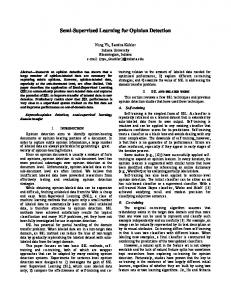
The values for Ah(i,1) and Ah(i,nj), i.e. the extreme windows of the line (left and right edges), take value zero. The outputs of the horizontal and vertical scans are two binary images, with the same dimensions as the matrix of window mean intensity values, where value ‘1’ means that the window possibly contains cracks. Each of the binary images is independently processed to identify connected component (with 8-neighbourhood), and only connected components with a total length higher than two are kept as candidate crack windows. The reasoning supporting this decision is that cracks present a linear development, unlike e.g., oil spots. The two binary images are then merged, and the length of the longest connect component is stored (llcc). A sample result obtained at this stage is show in Figure 2, considering the values 0.4 and 2.0 (selected after exhaustive testing) for the constants k1 and k2 in equations (2) and (4), respectively.

Figure 2 – Original image (on the left), automatically selected for the training set; binary image (on the right) with an llcc of 14.

Finally, all database images are sorted in decreasing order of their llcc values. Training images should be chosen from the top of this sorted list. Using this algorithm, all the images selected for the training set effectively contain cracks and images without cracks are positioned at the bottom of this sorted list. 2.3 Image normalization For reducing the effect of non-uniform illumination, an image normalization procedure is implemented. The aim is to compute a reference value for the road surface intensity, called base value (bv), corresponding to the mean of all pixel intensities for windows that are not expected to contain cracks, according to the algorithm presented in Section 2.2. A normalization factor (nf) for each window without cracks (i.e., with label ‘0’ in the merged binary matrix) is computed according to equation (6), where n takes values between 1


and the total number of windows in the image, and w’0’(n) stands for a window with label ‘0’ in the merged binary matrix. bv , (6) nf '0' (n) =

(

)

Mean intensity value w '0' (n )

Windows previously labeled with value ‘0’ are normalized by multiplying initial pixel intensities by the respective nf’0’ value. For instance, in a ‘0’ window with nf’0’ =1.05, a pixel with original intensity of 135 will take value 142 (1.05×135). For windows previously labeled with value ‘1’, i.e., windows likely to contain cracks, a different normalization procedure is followed. In this case, the mean value is computed using the means of its 8-neighbouring windows with label ‘0’, bv . (7) nf '1' (n) = Mean of '0' neighbours(n)

In case all neighbors have label ‘1’, the search for ‘0’ labeled windows is done on a larger neighborhood (e.g., 5×5). For instance, a window with label ‘1’ and mean intensity 110, with three label ‘0’ neighbors with means 148, 142 and 139, the denominator of (7) (i.e., the mean value of the ‘0’ neighbors) to consider would be 143, instead of 110. With this procedure, nf values for windows with label ‘1’ are similar to those of windows without cracks. After normalization, all the images will present a similar mean intensity value in road surface areas without cracks. 2.4 Feature extraction and normalization The features considered for the classification task are computed for the normalized images. They include the mean value of the image windows, organized into a matrix as described above, together with a standard deviation matrix, again computed for each image window. Finally, a top-hat filter is applied, replacing all pixels with intensities higher than bv, with value bv, and leaving picxels with intensity lower than bv unchanged. The 2D feature space is also normalized, to reduce the feature representation scattering between database images, in order to allow a better classification performance. The centroid of each database image’s two dimensional feature space is calculated, as well as a global centroid, based on the full set of points (all the images). For each individual image, the two dimensional feature space points are translated so that the respective centroid coincides with the global centroid. 3.

TRAINING AND CLASSIFICATION

This section describes the classification strategies being evaluated, which are based on two supervised learning approaches: parametric (Section 3.1) and nonparametric (Section 3.2). Parametric approaches are based on a bivariate class-conditional normal density, as it provides a good description of the data [5]. 3.1 Parametric learning and classification The measurements for each image (mean and standard deviation of pixel intensities within a window) compose a pattern vector x, representing a sample of the random variable X, taking values on a sample space X. For each element xi of vector x one possible class yi will be assigned, where Y is the

class set. Thus, the training set is: Τ = {(x1 , y1 )K ( x n , y n ) : x i ∈ ℜ 2 ; y i ∈ {c1 , c 2 }}, (8) where n is the number of vector x elements. Only two classes are used: windows without cracks (class c1) or windows with cracks (class c2). Since ground truth for the training set is known (the user selects windows with cracks in training images), the parameters for each of the two classes are learned from the measurements, according to [6]: 1 nm T 1 nm ˆ µˆ m = ∑ x m i and ∑m = n −1 ∑(xmi − µˆm )(xmi − µˆm ) , (9) i =1 n m i =1 m where µˆ m is the sample unbiased vector mean, Σˆ m is the sample unbiased covariance computed for each training image, m corresponds to the class identification, and nm is the total number of measurements for class m. The prior’s estimation for each class is computed according to the observed class frequencies: # measurements labeled c m . (10) P( y i = c m ) = # measurements for all classes

After parameter learning, a Bayesian classifier is used, based on the knowledge that an action is to be taken (classification of a window into one of the two classes) that minimizes its associated risk, symbolically represented by (11), which corresponds to a maximum a posteriori probability classifier, since a uniform cost function is used [7]. c1 p(x | y i = c1 )P( y i = c1 ) > p(x | y i = c 2 )P( y i = c 2 ) . < c2

(11)

This paper considers 3 ways to compute the decision boundary. The first one, denoted as linear, assumes a joint sample covariance matrix (Σ), with the boundary being computed by a weighted average (according to the class prior probabilities) of each class’ covariance matrix, which results in a linear decision boundary [7] [8], given by: α + xT β = 0 (12)

α = 2 ln

P ( yi = c2 ) − µ 2T ∑ −1 µ 2 + µ1T ∑ −1 µ1 P ( yi = c1 ) β = 2 ∑ −1 (µ 2 − µ1 )

(13) (14)

The second way to compute the decision boundary, denoted as quadratic, assumes a general covariance matrix resulting in the quadratic boundary [8] defined by: α + x T β + x Tϕ x = 0 (15) α = + ln ∑1 − ln ∑2 + 2 ln

P( yi = c2 ) − µ2T ∑−21 µ2 + µ1T ∑1−1 µ1 (16) P( yi = c1)

β = 2(∑ −2 1 µ 2 − ∑1−1 µ1 ) and

ϕ = − ∑ −21 + ∑1−1

(17) The third decision boundary, denoted as independent, is computed assuming independent features, i.e. the covariance matrices in (9) are now diagonal matrices, computed as ˆ ∑ = E x −µ x −µ , (18) ml ,l

and

[(

ml

ml

)( m

l

ml

)]

Σˆ ml ,k takes value zero whenever l ≠ k; E stands for the

expected value, and l and k are feature identifiers, taking value 1 or 2 for the no-cracks and cracks classes, respectively. Using these new covariance matrices, the equations


from (15) to (17) are used to compute the decision boundary. A sample result using the three types of decision boundaries computed using the training image shown in Figure 2 (left part), is illustrated in Figure 3.

when the training data is not homogeneous, i.e., it’s resolution is higher when the training data is more dense. The posterior probability density for an arbitrary test vector z is computed by [7][11]: km (22) n m V(z ) where km is the number of samples inside the volume V(z)— which represents a sphere centered in z—belonging to class m and nm is the total number of training samples belonging to class m. Thus, a measurement is classified into the class (c1 or c2) that contains more training measurements in the km neighborhood of z, since: mˆ = arg max pˆ (z | y = c )Pˆ ( y = c ) = arg max k , (23) pˆ (z | y i = c m ) ≈

Figure 3 –Three parametric decision boundaries computed over the training data set.

3.2 Non-parametric learning and classification This section deals with classifiers that operate when conditional probability distributions are unavailable. This is different from the parametric case, where the only unknowns were the probability density parameters modeling the data. In general, one advantage of non-parametric learning, when compared with parametric learning, is that not so much prior knowledge about the data to be processed is required, but a large amount of data is needed [9], although it can be reduced if certain constrains are incorporated [10]. Here, three non-parametric techniques are considered: Parzen windows, k-Nearest Neighbor and Fisher's Least Square Linear classifiers. The implemented Parzen algorithm for learning and classification follows the descriptions in [8][10]. Considering a labeled training vector x according with (8) and an unlabelled test set, the probability density estimation for an arbitrary test vector z is achieved by: pˆ (z | y i = c m ) =

 z−x 2    , (19) q 1 nm 1 exp − ∑  2 n m q =1 2π × fs 2 2 fs    14444 4244444 3 A

where A is a kernel that represents the knowledge about the distance between a test measurement z and the training measurement xq, corresponding to a Gaussian interpolation distance function, nm is the total number of measurements for class m and fs is a constant that controls the size of the kernel influence zone, computed such that it maximizes:

∑ ∑ ln( pˆ (x m,q | yi = c m )) ,

m =1, 2

{

i

m

i

m

}

m =1, 2

{ } m

where Pˆ ( yi = cm ) again represents the class priors according to (10). The aim of the Fischer’s linear classification strategy is to find the linear discriminant function between the two classes, which corresponds to the projection that maximizes the class separation [6][7]. Class separability is defined by: KT JBK

R( K ) =

, (24) KT JK K which is also denoted as the ratio of the between-class covariance matrix (JB) to the within-class covariance matrix (JK), defined as: J B = (µ1 − µ 2 )(µ1 − µ 2 )T , 2

J K = J K c + J K c , J K c = ∑ ( xi − µi )( xi − µi )T 1

2

i

(25) (26)

i =1

where µi denotes the vector mean for class i, computed according to (9) and xi is class i measurements vector data. An estimate of K is obtained maximizing (24) according to,  KT J K  Kˆ = argmax T B  . K J K K K  

(27)

Thus, a measurement from the test vector z, is classified into class c1 when y(xi)/y0 for y0=K.z (z classified into class c2 otherwise). A sample result using the three types of decision boundaries, computed using the training image shown in Figure 2 (left part), is illustrated in Figure 4.

2 nm

(20)

m =1q =1

where xm,q is the sample q of the class m which is left out by the leave-one-out method when computing the estimation of the posterior probability density. A measurement is classified into the class ck which has the maximum posterior probability: (21) mˆ = argmax pˆ (z | y = c )Pˆ ( y = c ) , m =1, 2

[

i

m

i

m

]

where Pˆ ( yi = cm ) represents class priors according to (10). For k-Nearest Neighbors Classification (k-nn), the estimated posterior probability density may have different resolutions

Figure 4 –Three non-parametric decision boundaries computed over the same training data set. For k-nn, the boundary shown corresponds to a neighborhood of 1.


4.

EXPERIMENTAL RESULTS AND PERFORMANCE EVALUATION

The presented classification strategies are evaluated over a test set composed by real flexible pavement surface images, containing cracks with linear development, acquired during a survey over a Portuguese road, for which ground truth data has been manually obtained. Part of the algorithmic development was supported by the PRtools [12] toolbox. Figure 5 shows results for one test image, using the considered classifiers. For the k-nn strategy, one nearest neighbor (1-nn) is considered, as this is the neighborhood that optimizes the leave-one-out error over the test set.

It is important to note that although the use of k-nn classifier produces good results (see PC and Recall), it may be difficult to obtain a fixed neighborhood size. For different training images, values between 1 and 10 were observed, with a mean value of 4. Using a small neighborhood may produce some over fitting problems, with the decision boundary adapted to the training set, producing worst generalization performance of the classifier, when the test set is processed. Additionally, all the classifiers seem to perform very well according to false positives detection (i.e., windows without cracks being classified as containing cracks), with the corresponding computed errors very close to zero. 5.

CONCLUSIONS

In this paper an automatic training image selection procedure is proposed. The proposed technique is very effective on managing the data (images) to construct training and test sets. Additionally, six supervised classification strategies (three parametric and three non-parametric) are analyzed. All six obtain an acceptable performance, with parametric classifiers, especially the quadratic one, achieving the best classification results. Future developments may consider a reject-option and a non uniform loss function, since false positive detections have less impact than false negatives detection. Also a deeper study of windows size, to maximize class separability, will be performed. Figure 5 – Experimental results for a test image. Top (left to right): original, ground truth classification. 2nd line (parametric classifiers): linear, quadratic, classifier with independent features. 3rd line (nonparametric): Parzen windows, 1-nn nearest neighbors and Fischer.

An evaluation of the different strategies, taking into account ground truth data, is included in Table 1. A global Error-rate is computed (classification error for classes c1 and c2), as well as some metrics related only to windows with cracks: Crack Error-rate, Precision, Recall and a Performance Criterion (PC) reflecting the overall classifier performance [13]. Table 1 – Results for the detection of windows with cracks. Strategy Linear Quadratic Independ. Parzen k-nn Fischer

Global Error-rate 0.68% 0.64% 0.85% 0.73% 0.78% 1.00%

Crack Error-rate 8.90% 2.96% 6.87% 10.79% 5.38% 15.45%

Precision

Recall

PC

97.1% 92.5% 92.4% 98.2% 92.5% 98.1%

91.2% 97.0% 93.1% 89.2% 94.6% 84.6%

94.0% 94.7% 92.7% 93.3% 93.5% 90.7%

The best overall classifier performance is achieved by the quadratic classifier (see PC values), also denoted by the best Recall value, meaning that this classifier produces the best true positive detection performance. An interesting observation is that the features used seem to have some degree of dependence, which can be seen by comparing the quadratic and the independent parametric classifier results, i.e., a worst classification performance is achieved when a diagonal covariance matrix is assumed. The use of parametric classifiers seems to be a good strategy, producing better PC values, notably taking into account that Recall is more important than Precision for this type of application.

REFERENCES [1] H. Cheng and M. Miyojim, “Automatic Pavement Distress Detection System”, Journal of Information Sciences 108, Elsevier, pp. 219-240, July 1998. [2] Y. Huang and B. Xu: “Automatic Inspection of Pavement Cracking Distress”. Journal of Electronic Imaging. Society for Imaging Science and Technology, USA 2006. [3] K. Wang, “Design and Implementations of Automated Systems for Pavement Surface Distress Survey”, Journal of Infrastructure Systems, ASCE, USA, Vol. 6, March, 2000. [4] H. .Zhang and Q. Wang, “Use of Artificial Living System for Pavement Distress Survey”, 30th Annual Conference of the IEEE Industrial Electronics Society, Korea, pp. 2486-2490 Vol.3, 2004. [5] H. Oliveira and P.L. Correia, Automatic Crack Pavement Detection Using a Bayesian Stochastic Pattern Recognition System, RECPAD2007, Portugal, 2007. [6] C. Bishop, Pattern Recognition and Machine Learning, Springer, USA, 2006. [7] R. Duda, P. Hart and D. Stork, Pattern Classification, John Wiley & Sons, Canada, 2001. [8] F. Heijden, R. Duin, D. Ridder and D. Tax, Classification, Parameter Estimation and State Estimation – an engineering approach using MatLab, John Wiley & Sons, England, 2004. [9] A. Webb, Statistical Pattern Recognition – 2th edition, John Wiley & Sons, England, 2002. [10] K. Fukunaga , Introduction to Statistical Pattern Recognition – 2th edition, Morgan Kaufman, USA,1990. [11] S Theodoridis and K. Foutroumbas., Pattern Recognition – 2th edition, Elsevier – Academic Press, USA, 2003. [12] R. Duin, P. Juszczak, P. Paclik, E. Pekalska, D. Ridder, D. Tax: PRTools 4 - A MatLab Toolbox for Pattern Recognition – version 4.0.23, http://www.prtools.org/, Netherlands, 2004. [13] D. Tax: Data Description Toolbox, http://ict.ewi.tudelft.nl/ ~davidt/dd_tools.html, Netherlands, 2006.