We simulated GWAS effect sizes as outlined in section 3.1 where the ... current methods, we conduct a modest comparison against COLOC. We simulated 100 ...
Supplementary Figures: A unifying framework for joint trait analysis under a non-infinitesimal model Ruth Johnson1 , Huwenbo Shi2 , Bogdan Pasaniuc∗2,3,4 , and Sriram Sankararaman∗1,2,3 1
Department of Computer Science, University of California, Los Angeles, Los Angeles, CA 90024, USA 2 Bioinformatics Interdepartmental Program, University of California, Los Angeles, Los Angeles, CA 90024, USA 3 Department of Human Genetics, David Geffen School of Medicine, University of California, Los Angeles, Los Angeles, CA 90024, USA 4 Department of Pathology and Laboratory Medicine, David Geffen School of Medicine, University of California, Los Angeles, Los Angeles, CA 90024, USA
1
Pruning window (K) no pruning 1KB 5KB 10KB 20KB 30KB 40KB 50KB
Mean SD Mean SD Mean SD Mean SD Mean SD Mean SD Mean SD Mean SD
p00 (0.99)
p10 (0.0025)
p01 (0.0025)
p11 (0.0050)
0.986472 0.09199 0.976628 0.1369 0.999993 9.391e-06 0.999992 9.811e-06 0.999991 1.088e-05 0.999985 1.307e-05 0.999982 1.335e-05 0.999979 1.327e-05
2.591e-06 7.685e-06 2.515e-06 7.53e-06 2.432e-06 3.854e-06 2.56e-06 3.915e-06 2.985e-06 4.091e-06 5.208e-06 5.205e-06 6.177e-06 5.474e-06 6.908e-06 5.287e-06
0.01352 0.09199 0.02337 0.1369 2.582e-06 4.091e-06 2.631e-06 3.978e-06 3.195e-06 4.6e-06 5.18e-06 5.689e-06 6.16e-06 5.923e-06 6.961e-06 6.013e-06
3.165e-06 1.28e-05 3.168e-06 1.28e-05 2.43e-06 3.898e-06 2.763e-06 4.043e-06 3.259e-06 4.249e-06 5.152e-06 5.061e-06 6.282e-06 5.644e-06 6.933e-06 6.157e-06
Table 1: To model a realistic LD structure, we used SNPs from 1000 Genomes to compute the LD for approximately 2,000 independent LD blocks. We simulated GWAS effect sizes as outlined in section 3.1 where the heritabilities for each trait was set to h21 = 0.50 and h22 = 0.50, genetic correlation ρ = 0. We varied the non-overlapping window length, K, to assess the minimal window size necessary to create a subset of approximately independent SNPs. Our results demonstrate that using a 5KB window gives more precise estimates while retaining the highest number of SNPs.
2
one causal multiple causals
p10
Simulation parameters 1 p10 = 0, p01 = 0, p11 = M = 0.01, p01 = 0.01, p11 = 0.01
H0 14.29% 4.76%
H1 17.84% 13.71%
H2 16.55% 9.10%
H3 0.13% 63.27%
H4 51.19% 9.17%
Table 2: To empirically demonstrate the benefit of the relaxed assumptions of UNITY as compared to current methods, we conduct a modest comparison against COLOC. We simulated 100 regions of M=500 SNPs under two simulation frameworks with the proportion parameters outlined in the second column and h21 = 0.00125, h22 = 0.00125, ρ = 0, N1 = 100, 000, N2 = 100, 000. COLOC calculates the posterior probability of a region corresponding to one of the 5 hypothesis - H0: no associated with either trait, H1: association with only trait 1, H2: association with only trait 2, H3: association with both traits driven by two independent SNPs, and H4: association with both trait 1 and trait 2 driven by one shared SNP (i.e. colocalized). We report the average posterior probability calculated over the 100 regions for each of the hypotheses.
3
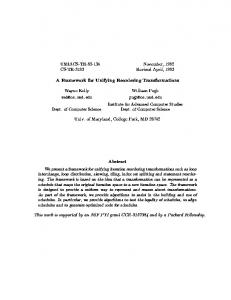
Runtime verus number of SNPs ●
5.5 5.0
Seconds per iteration
4.5 4.0 3.5 3.0 2.5 2.0 1.5 1.0
●
0.5 0.0
●
● ● ●
0e+00
1e+06
2e+06
3e+06
4e+06
5e+06
Number of SNPs Figure 1: The complexity of our algorithm is O(M ), where M is the number of SNPs for each trait. We varied the total number of SNPs from 100 to 5,000,000 and then performed MCMC for 100 iterations and recorded the total amount of time necessary for sampling. This total time divided by the number of iterations is reported on the y-axis.
4
Proportion of causal SNPS in Trait 1 (p10)
Proportion of causal SNPs in Trait 2 (p01) ●
●
●
●
●
●
●
●
●
0.4
0.2
0.6
Estimated proportion of SNPs
0.6
Estimated proportion of SNPs
0.6
Estimated proportion of SNPs
Proportion of shared causal SNPS (p11)
●
●
0.4
0.2
●
1K
25K
0.2
●
●
● ●
0.0
●
0.4
●
●
50K
100K
Sample size (N1=N2)
● ●
●
●
50K
100K
0.0
250K
1K
25K
Sample size (N1=N2)
● ●
0.0
250K
1K
25K
●
●
50K
100K
250K
Sample size (N1=N2)
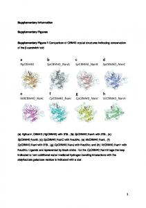
Figure 2: To assess the role of sample size in our inference, we performed simulations where we varied the number of individuals from 1,000 to 250,000. We simulated 100,000 SNPs where h21 = 0.25, h22 = 0.25, ρ = 0.25, p10 , p01 , p11 = 0.01. This was repeated for 100 independent simulations, and we report the posterior means for each simulation in the plots above. Note that the variance of our estimates increases when the sample size is under 25,000 individuals. We recommend users have at least 50,000 individuals for each trait to yield robust estimates.
5
N1=100K, N2=100K, M=100K, h1=.25, h2=.25, rho=0 ● ●
Estimated proportion of SNPs
0.75
0.50
0.25
● ●
0.00
p00
p10
p01
p11
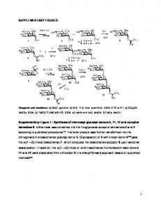
Figure 3: To assess whether our estimates are invariant to an unequal trait-specific proportion of causal SNPs, we performed simulations where p10 6= p01 . This was repeated for 100 independent simulations, and we report the posterior means for each simulation in the plots above. .
6
N1=100K, N2=100K, M=100K, h1=.40, h2=.20, rho=0 ● ● ●
Estimated proportion of SNPs
0.75
0.50
0.25
● ●
0.00
p00
p10
p01
p11
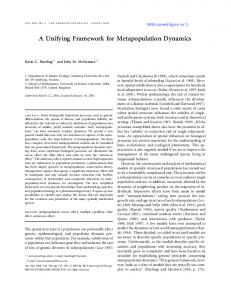
Figure 4: To assess whether our estimates are invariant to differing levels of heritability between traits, we performed simulations where h21 6= h22 . This was repeated for 100 independent simulations, and we report the posterior means for each simulation in the plots above.
7