Support for Feature Orirnted Programming

Support for Feature Orirnted Programming Autonomic Elastic Clouds

PDF generated using the open source mwlib toolkit. See http://code.pediapress.com/ for more information. PDF generated at: Sun, 29 Jan 2012 09:24:53 UTC

Contents Articles Presentation–abstraction–control

1

Common Lisp

3

Oz (programming language)

26

Constraint programming

31

Functional logic programming

34

Lazy evaluation

35

Eager evaluation

39

Prolog

40

Resolution (logic)

53

Propositional calculus

57

First-order logic

74

Programming paradigm

93

Language-oriented programming

96

General-purpose programming language

98

Domain-specific language

99

JetBrains MPS

106

XL (programming language)

108

Forth (programming language)

114

APL (programming language)

127

Automatic programming

141

Intentional programming

143

Time-driven programming

147

Function-level programming

147

Value-level programming

149

Metaprogramming

150

Template metaprogramming

152

Reflection (computer programming)

158

Attribute-oriented programming

165

Nondeterministic programming

167

Policy-based design

168

Feature-oriented programming

171

Declarative programming

176

Mathematical logic

178

Compiler optimization

191

Service-oriented modeling

202

Grammar-oriented programming

213

Dialecting

214

Semantic-oriented programming

214

Subject-oriented programming

216

Separation of concerns

219

Role-oriented programming

223

Service-oriented architecture

225

Reactive programming

240

Agent-oriented programming

243

Automata-based programming

244

Component-based software engineering

254

Flow-based programming

259

Pipeline programming

269

Concurrent computing

269

Relativistic programming

273

Data-driven programming

274

Problem-oriented development

275

Automated planning and scheduling

276

Strategy

278

STRIPS

281

Action description language

283

Reactive planning

287

Scheduling (computing)

290

Planning

298

Planning Domain Definition Language

302

Intelligent agent

305

Belief–desire–intention software model

309

Procedural reasoning system

313

Metaknowledge

316

Domain-specific modeling

317

Program transformation

319

FermaT Transformation System

320

Transformation language

321

Semantic translation

322

Model-driven engineering

323

Model-driven architecture

326

Data transformation

331

Modeling language

333

Reason

337

Metacognition

352

Automated reasoning

357

Category:Logic in computer science

360

Deductive reasoning

360

Inductive reasoning

362

Abductive reasoning

367

Analogy

379

Fallacy

389

Semantics of programming languages

397

Semantic reasoner

399

Inference

402

Axiom

406

Entailment

413

Inference engine

419

Description language

420

Ontology language

421

Probabilistic logic network

422

Backward chaining

424

Description logic

425

Rule of inference

435

Glue semantics

437

Context-free grammar

438

Linear logic

449

Discourse representation theory

456

Intensional logic

458

Natural semantic metalanguage

460

Lexical functional grammar

463

Subject (grammar)

465

Predicate (grammar)

469

Object (grammar)

473

Feature (linguistics)

475

Grammatical tense

476

Transformational grammar

481

Dependency grammar

486

Morphology (linguistics)

491

Phonology

498

Non-configurational language

505

Monotonic function

507

Monotonicity of entailment

511

Logic

512

Non-monotonic logic

524

Reification (computer science)

526

Reification (knowledge representation)

530

Reification (linguistics)

531

Metaobject

532

Type introspection

533

First-class citizen

539

Run time (program lifecycle phase)

541

Polymorphism (computer science)

542

Mixin

546

Trait (computer programming)

550

Self (programming language)

551

Moose (Perl)

557

Joose (framework)

560

Fortress (programming language)

562

Concept-oriented design

564

Concept programming

565

Abstract syntax tree

567

Artefaktur

569

Semantic resolution tree

569

Abstract data type

569

Aspect-oriented programming

577

Concept-oriented model

586

Aspect-oriented software development

591

Abstraction (computer science)

602

Lua (programming language)

609

Smalltalk

619

Procedural programming

633

Imperative programming

636

Structured programming

638

Modular programming

642

Separation of presentation and content

643

Concern (computer science)

645

Cross-cutting concern

646

Distributed AOP

648

Dependency injection

649

Delegation (programming)

656

Prototype-based programming

661

Feature-driven development

666

Metamodeling

675

Model transformation language

678

Meta-process modeling

680

Metadata modeling

689

Metalanguage

692

OCaml

695

Hygienic macro

704

Template Haskell

708

Aspect weaver

709

Partial evaluation

714

Self-modifying code

715

Nemerle

721

Stratego/XT

729

DMS Software Reengineering Toolkit

731

Inferential programming

733

Interpreted language

733

Comparison of code generation tools

736

Machine learning

741

Genetic programming

747

Artificial intelligence

753

Evolution

780

Generic programming

809

ECMAScript

827

List of reflective programming languages and platforms

835

Software inspection

836

Groovy (programming language)

838

Scripting language

841

Scala (programming language)

845

Clojure

850

Grails (framework)

855

Ruby (programming language)

862

JRuby

877

Python (programming language)

884

Perl

898

SALSA (programming language)

912

MultiLisp

912

Joule (programming language)

913

Limbo (programming language)

915

Erlang (programming language)

917

Eiffel (programming language)

927

Curry (programming language)

941

Alef (programming language)

944

Ada (programming language)

946

ML (programming language)

959

Standard ML

962

Alice (programming language)

976

CHAIN (programming language)

977

AspectJ

978

Chapel (programming language)

981

Fourth-generation programming language

982

Nomad software

987

Monad (functional programming)

991

Syntactic sugar

1007

Mutator method

1009

Lambda calculus

1019

Saccharin

1035

Cayenne (programming language)

1040

Comparison of programming paradigms

1041

CoffeeScript

1047

Cappuccino (application development framework)

1050

Ext JS

1052

jQuery

1055

Definite clause grammar

1061

Grammar induction

1065

Syntactic pattern recognition

1067

Formal grammar

1068

Decision rules

1073

Evolutionary algorithm

1073

Artificial grammar learning

1076

Greedy algorithm

1076

Algorithmic composition

1079

Grammatical aspect

1085

Lexical aspect

1094

Continuous and progressive aspects

1096

Perfective aspect

1105

Grammatical evolution

1106

Evolutionary computation

1108

Particle swarm optimization

1111

Combinatorial optimization

1116

Solver

1118

Heuristic

1119

Social proof

1124

Social information architecture

1129

Social software (social procedure)

1131

Sociotechnical systems

1133

Performance

1140

Goal-oriented

1142

Goal-oriented Requirements Language

1149

Modeling perspective

1151

Resource mobilization

1153

Motivation

1155

Extended Enterprise Modeling Language

1166

i*

1170

Actor modeling

1173

Business Motivation Model

1174

KAOS (software development)

1175

Goal modeling

1176

Unified Modeling Language

1178

Use case

1187

Goal

1191

Soft goal

1193

Task analysis

1194

Resource (computer science)

1196

Actor

1197

Requirements engineering

1201

Object-capability model

1202

Design pattern

1205

System Architect (software)

1207

Object-relational mapping

1212

e (verification language)

1215

Annotation

1221

Open Vulnerability and Assessment Language

1223

Design by contract

1224

Precondition

1229

Postcondition

1230

Side effect (computer science)

1231

Invariant (computer science)

1233

Hoare logic

1235

Formal methods

1238

Defensive programming

1242

Program refinement

1247

Test-driven development

1248

Evaluation strategy

1254

Expression (computer science)

1259

Evaluation approaches

1260

Software assurance

1265

References Article Sources and Contributors

1268

Image Sources, Licenses and Contributors

1292

Article Licenses License

1296

Presentation–abstraction–control

Presentation–abstraction–control Presentation–abstraction–control (PAC) is a software architectural pattern. It is an interaction-oriented software architecture, and is somewhat similar to model–view–controller (MVC) in that it separates an interactive system into three types of components responsible for specific aspects of the application's functionality. The abstraction component retrieves and processes the data, the presentation component formats the visual and audio presentation of data, and the control component handles things such as the flow of control and communication between the other two components .[1] In contrast to MVC, PAC is used as a hierarchical structure of agents, each consisting of a triad of presentation, abstraction and control parts. The agents (or triads) communicate with each other only through the control part of each triad. It also differs from MVC in that within each triad, it completely insulates the presentation (view in MVC) and the abstraction (model in MVC), this provides the option to separately multithread the model and view which can give the user experience of very short program start times, as the user interface (presentation) can be shown before the abstraction has fully initialized.

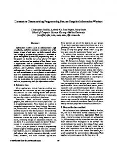
Hierarchical model–view–controller (HMVC) A variation of MVC similar to PAC was published in an article[2] in JavaWorld Magazine, the authors apparently unaware[3] of PAC which was published 13 years earlier. The main difference between HMVC and PAC is that HMVC is less strict in that it allows the view and model of each agent to communicate directly, thus bypassing the controller. The structure of an application with PAC. The controller has some oversight. The controller selects the model and then selects the view, so there is an approval mechanism by the controller. The model prevents the view from accessing the data source directly.

References • Coutaz, Joëlle (1987). "PAC: an Implementation Model for Dialog Design" [4]. In H-J. Bullinger, B. Shackel (ed.). Proceedings of the Interact'87 conference, September 1–4, 1987, Stuttgart, Germany. North-Holland. pp. 431–436. • Frank Buschmann, Regine Meunier, Hans Rohnert, Peter Sommerlad, Michael Stal (1996). Pattern-Oriented Software Architecture Vol 1: A System of Patterns. John Wiley and Sons. pp. 145–168. ISBN 0-471-95869-7. • Gaëlle Calvary; Joëlle Coutaz, Laurence Nigay (1997). "From Single-User Architectural Design to PAC*: a Generic Software Architecture Model for CSCW" [5]. In Pemberton, Steven (ed.). Proceedings of the ACM CHI 97 Human Factors in Computing Systems Conference. March 22–27, 1997, Atlanta, Georgia.. pp. 242–249. • Joëlle Coutaz (1997). "PAC-ing the Architecture of Your User Interface" [6]. DSV-IS’97, 4th Eurographics Workshop on Design, Specification and Verification of Interactive Systems. Springer Verlag. pp. 15–32.

1

Presentationabstractioncontrol • Markopoulos, Panagiotis (1997) (pdf). A compositional model for the formal specification of user interface software [7]. PhD thesis, Queen Mary and Westfield College, University of London. p. 26. Retrieved 2006-05-25. • Paris Avgeriou; Uwe Zdun (2005). "Architectural patterns revisited – a pattern language" [8]. Proceedings of 10th European Conference on Pattern Languages of Programs (EuroPlop 2005), Irsee, Germany, July 2005. pp. 1–39.

Notes [1] Kai, Qian (2009). "Interaction-oriented Software Architectures". Software Architecture and Design Illuminated. Jones and Bartlett Illuminated. pp. 200. ISBN 9780763754204. [2] Jason Cai, Ranjit Kapila, and Gaurav Pal (July 2000). "HMVC: The layered pattern for developing strong client tiers" (http:/ / www. javaworld. com/ javaworld/ jw-07-2000/ jw-0721-hmvc. html). JavaWorld. . Retrieved 2006-05-25. [3] "TP" (2000). "Is HMVC PAC? (letter to the editor)" (http:/ / web. archive. org/ web/ 20050205080537/ http:/ / www. javaworld. com/ javaworld/ jw-09-2000/ jw-0908-letters. html). JavaWorld. Archived from the original (http:/ / www. javaworld. com/ javaworld/ jw-09-2000/ jw-0908-letters. html) on 2005-02-05. . Retrieved 2006-05-25. [4] http:/ / www. interaction-design. org/ references/ conferences/ interact_87_-_2nd_ifip_international_conference_on_human-computer_interaction. html [5] http:/ / www1. acm. org/ sigs/ sigchi/ chi97/ proceedings/ paper/ jcc. htm [6] http:/ / iihm. imag. fr/ publs/ 1997/ DSVIS97_PACing. pdf [7] http:/ / www. idemployee. id. tue. nl/ p. markopoulos/ downloadablePapers/ PhDThesisPanosMarkopoulos. pdf [8] http:/ / www. daimi. au. dk/ MultiCore/ attachment/ wiki/ StudyGroup08/ Plan/

External links • Architectural outline for the game Warcraft as it might be implemented using the PAC Architectural Pattern: Programming of the application PACcraft:Architecture (http://web.archive.org/web/20070106050112/http:// iihm.imag.fr/nigay/ENSEIG/RICM3/siteWebRICM/TPS/TP2/TP2_architecture.html) (in french) • Pattern:Presentation-Abstraction-Control (http://www.vico.org/pages/PatronsDisseny/Pattern Presentation Abstra/) (pattern description) • PAC description in the Portland Pattern Repository (http://c2.com/cgi/wiki?PresentationAbstractionControl) • WengoPhone is a free software VoIP application that is written using the PAC design pattern. • description of PAC (http://web.archive.org/web/20070212210300/http://dev.openwengo.org/trac/ openwengo/trac.cgi/wiki/PAC) and motivation for use in WengoPhone. • demonstration code (http://web.archive.org/web/20070218041137/http://dev.openwengo.org/trac/ openwengo/trac.cgi/browser/playground/demopac), courtesy of the OpenWengo community. • HMVC: The layered pattern for developing strong client tiers (http://www.javaworld.com/javaworld/ jw-07-2000/jw-0721-hmvc.html?page=2)

2

Common Lisp

3

Common Lisp Common Lisp Paradigm(s)

Multi-paradigm: procedural, functional, object-oriented, meta, reflective, generic

Appeared in

1984, 1994 for ANSI Common Lisp

Developer

ANSI X3J13 committee

Typing discipline

dynamic, strong

Scope

lexical, optionally dynamic

Major implementations

Allegro CL, ABCL, CLISP, Clozure CL, CMUCL, Corman Common Lisp, ECL, GCL, LispWorks, Movitz, Scieneer CL, SBCL, Symbolics Common Lisp

Dialects

CLtL1, CLtL2, ANSI Common Lisp

Influenced by

Lisp, Lisp Machine Lisp, MacLisp, Scheme, InterLisp

Influenced

Clojure, Dylan, Emacs Lisp, EuLisp, Java, ISLISP, SKILL, Stella, SubL

OS

Cross-platform

Website

common-lisp.net

Family

Lisp

[1]

Common Lisp, commonly abbreviated CL, is a dialect of the Lisp programming language, published in ANSI standard document ANSI INCITS 226-1994 (R2004), (formerly X3.226-1994 (R1999)).[2] From the ANSI Common Lisp standard the Common Lisp HyperSpec has been derived[3] for use with web browsers. Common Lisp was developed to standardize the divergent variants of Lisp (though mainly the MacLisp variants) which predated it, thus it is not an implementation but rather a language specification. Several implementations of the Common Lisp standard are available, including free and open source software and proprietary products. Common Lisp is a general-purpose, multi-paradigm programming language. It supports a combination of procedural, functional, and object-oriented programming paradigms. As a dynamic programming language, it facilitates evolutionary and incremental software development, with iterative compilation into efficient run-time programs. It also supports optional type annotation and casting, which can be added as necessary at the later profiling and optimization stages, to permit the compiler to generate more efficient code. For instance, fixnum can hold an unboxed integer in a range supported by the hardware and implementation, permitting more efficient arithmetic than on big integers or arbitrary precision types. Similarly, the compiler can be told on a per-module or per-function basis which type safety level is wanted, using optimize declarations. Common Lisp includes CLOS, an object system that supports multimethods and method combinations. It is extensible through standard features such as Lisp macros (compile-time code rearrangement accomplished by the program itself) and reader macros (extension of syntax to give special meaning to characters reserved for users for this purpose). Though Common Lisp is not as popular as some non-Lisp languages, many of its features have made their way into other, more widely used programming languages and systems (see Greenspun's Tenth Rule).

Common Lisp

4

Syntax Common Lisp is a dialect of Lisp; it uses S-expressions to denote both code and data structure. Function and macro calls are written as lists, with the name of the function first, as in these examples: (+ 2 2)

; adds 2 and 2, yielding 4.

(defvar *x*)

; Ensures that a variable *x* exists, ; without giving it a value. The asterisks are part

of ; the name. The symbol *x* is also hereby endowed with ; the property that subsequent bindings of it are dynamic, (setf *x* 42.1) 42.1

; rather than lexical. ; sets the variable *x* to the floating-point value

;; Define a function that squares a number: (defun square (x) (* x x)) ;; Execute the function: (square 3) ; Returns 9 ;; the 'let' construct creates a scope for local variables. Here ;; the variable 'a' is bound to 6 and the variable 'b' is bound ;; to 4. Inside the 'let' is a 'body', where the last computed value is returned. ;; Here the result of adding a and b is returned from the 'let' expression. ;; The variables a and b have lexical scope, unless the symbols have been ;; marked as special variables (for instance by a prior DEFVAR). (let ((a 6) (b 4)) (+ a b)) ; returns 10

Data types Common Lisp has many data types—more than many other languages.

Scalar types Number types include integers, ratios, floating-point numbers, and complex numbers.[4] Common Lisp uses bignums to represent numerical values of arbitrary size and precision. The ratio type represents fractions exactly, a facility not available in many languages. Common Lisp automatically coerces numeric values among these types as appropriate. The Common Lisp character type is not limited to ASCII characters. Most modern implementations allow Unicode characters.[5] The symbol type is common to Lisp languages, but largely unknown outside them. A symbol is a unique, named data object with several parts: name, value, function, property list and package. Of these, value cell and function cell are

Common Lisp the most important. Symbols in Lisp are often used similarly to identifiers in other languages: to hold the value of a variable; however there are many other uses. Normally, when a symbol is evaluated, its value is returned. Some symbols evaluate to themselves, for example all symbols in the keyword package are self-evaluating. Boolean values in Common Lisp are represented by the self-evaluating symbols T and NIL. Common Lisp has namespaces for symbols, called 'packages'. A number of functions are available for rounding scalar numeric values in various ways. The function round rounds the argument to the nearest integer, with halfway cases rounded to even The functions truncate, floor, and ceiling round towards zero, down, or up respectively. All these functions return the discarded fractional part as a secondary value. For example, (floor -2.5) yields -3, 0.5; (ceiling -2.5) yields -2, -0.5; (round 2.5) yields 2, 0.5; and (round 3.5) yields 4, -0.5.

Data structures Sequence types in Common Lisp include lists, vectors, bit-vectors, and strings. There are many operations which can work on any sequence type. As in almost all other Lisp dialects, lists in Common Lisp are composed of conses, sometimes called cons cells or pairs. A cons is a data structure with two slots, called its car and cdr. A list is a linked chain of conses. Each cons's car refers to a member of the list (possibly another list). Each cons's cdr refers to the next cons—except for the last cons, whose cdr refers to the nil value. Conses can also easily be used to implement trees and other complex data structures; though it is usually advised to use structure or class instances instead. It is also possible to create circular data structures with conses. Common Lisp supports multidimensional arrays, and can dynamically resize arrays if required. Multidimensional arrays can be used for matrix mathematics. A vector is a one-dimensional array. Arrays can carry any type as members (even mixed types in the same array) or can be specialized to contain a specific type of members, as in a vector of integers. Many implementations can optimize array functions when the array used is type-specialized. Two type-specialized array types are standard: a string is a vector of characters, while a bit-vector is a vector of bits. Hash tables store associations between data objects. Any object may be used as key or value. Hash tables, like arrays, are automatically resized as needed. Packages are collections of symbols, used chiefly to separate the parts of a program into namespaces. A package may export some symbols, marking them as part of a public interface. Packages can use other packages. Structures, similar in use to C structs and Pascal records, represent arbitrary complex data structures with any number and type of fields (called slots). Structures allow single-inheritance. Classes are similar to structures, but offer more dynamic features and multiple-inheritance. (See CLOS). Classes have been added late to Common Lisp and there is some conceptual overlap with structures. Objects created of classes are called Instances. A special case are Generic Functions. Generic Functions are both functions and instances.

Functions Common Lisp supports first-class functions. For instance, it is possible to write functions that take other functions as arguments or return functions as well. This makes it possible to describe very general operations. The Common Lisp library relies heavily on such higher-order functions. For example, the sort function takes a relational operator as an argument and key function as an optional keyword argument. This can be used not only to sort any type of data, but also to sort data structures according to a key. ;; Sorts the list using the > and < function as the relational operator. (sort (list 5 2 6 3 1 4) #'>) ; Returns (6 5 4 3 2 1) (sort (list 5 2 6 3 1 4) #'. Conversely, to call a function passed in such a way, one would use the funcall operator on the argument. Scheme's evaluation model is simpler: there is only one namespace, and all positions in the form are evaluated (in any order) -- not just the arguments. Code written in one dialect is therefore sometimes confusing to programmers more experienced in the other. For instance, many Common Lisp programmers like to use descriptive variable names such as list or string which could cause problems in Scheme, as they would locally shadow function names. Whether a separate namespace for functions is an advantage is a source of contention in the Lisp community. It is usually referred to as the Lisp-1 vs. Lisp-2 debate. Lisp-1 refers to Scheme's model and Lisp-2 refers to Common Lisp's model. These names were coined in a 1988 paper by Richard P. Gabriel and Kent Pitman, which extensively compares the two approaches.[6]

7

Common Lisp

Other types Other data types in Common Lisp include: • Pathnames represent files and directories in the filesystem. The Common Lisp pathname facility is more general than most operating systems' file naming conventions, making Lisp programs' access to files broadly portable across diverse systems. • Input and output streams represent sources and sinks of binary or textual data, such as the terminal or open files. • Common Lisp has a built-in pseudo-random number generator (PRNG). Random state objects represent reusable sources of pseudo-random numbers, allowing the user to seed the PRNG or cause it to replay a sequence. • Conditions are a type used to represent errors, exceptions, and other "interesting" events to which a program may respond. • Classes are first-class objects, and are themselves instances of classes called metaobject classes (metaclasses for short). • Readtables are a type of object which control how Common Lisp's reader parses the text of source code. By controlling which readtable is in use when code is read in, the programmer can change or extend the language's syntax.

Scope Like programs in many other programming languages, Common Lisp programs make use of names to refer to variables, functions, and many other kinds of entities. Named references are subject to scope. The association between a name and the entity which the name refers to is called a binding. Scope refers to the set of circumstances in which a name is determined to have a particular binding.

Determiners of scope The circumstances which determine scope in Common Lisp include: • the location of a reference within an expression. If it's the leftmost position of a compound, it refers to a special operator or a macro or function binding, otherwise to a variable binding or something else. • the kind of expression in which the reference takes place. For instance, (GO X) means transfer control to label X, whereas (PRINT X) refers to the variable X. Both scopes of X can be active in the same region of program text, since tagbody labels are in a separate namespace from variable names. A special form or macro form has complete control over the meanings of all symbols in its syntax. For instance in (defclass x (a b) ()), a class definition, the (a b) is a list of base classes, so these names are looked up in the space of class names, and x isn't a reference to an existing binding, but the name of a new class being derived from a and b. These facts emerge purely from the semantics of defclass. The only generic fact about this expression is that defclass refers to a macro binding; everything else is up to defclass. • the location of the reference within the program text. For instance, if a reference to variable X is enclosed in a binding construct such as a LET which defines a binding for X, then the reference is in the scope created by that binding. • for a variable reference, whether or not a variable symbol has been, locally or globally, declared special. This determines whether the reference is resolved within a lexical environment, or within a dynamic environment. • the specific instance of the environment in which the reference is resolved. An environment is a run-time dictionary which maps symbols to bindings. Each kind of reference uses its own kind of environment. References to lexical variables are resolved in a lexical environment, et cetera. More than one environment can be associated with the same reference. For instance, thanks to recursion or the use of multiple threads, multiple activations of the same function can exist at the same time. These activations share the same program text, but each has its own lexical environment instance.

8

Common Lisp To understand what a symbol refers to, the Common Lisp programmer must know what kind of reference is being expressed, what kind of scope it uses if it is a variable reference (dynamic versus lexical scope), and also the run-time situation: in what environment is the reference resolved, where was the binding introduced into the environment, et cetera.

Kinds of environment Global Some environments in Lisp are globally pervasive. For instance, if a new type is defined, it is known everywhere thereafter. References to that type look it up in this global environment. Dynamic One type of environment in Common Lisp is the dynamic environment. Bindings established in this environment have dynamic extent, which means that a binding is established at the start of the execution of some construct, such as a LET block, and disappears when that construct finishes executing: its lifetime is tied to the dynamic activation and deactivation of a block. However, a dynamic binding is not just visible within that block; it is also visible to all functions invoked from that block. This type of visibility is known as indefinite scope. Bindings which exhibit dynamic extent (lifetime tied to the activation and deactivation of a block) and indefinite scope (visible to all functions which are called from that block) are said to have dynamic scope. Common Lisp has support for dynamically scoped variables, which are also called special variables. Certain other kinds of bindings are necessarily dynamically scoped also, such as restarts and catch tags. Function bindings cannot be dynamically scoped using FLET (which only provides lexically scoped function bindings), but function objects (a first-level object in Common Lisp) can be assigned to dynamically scoped variables, bound using LET in dynamic scope, then called using FUNCALL or APPLY. Dynamic scope is extremely useful because it adds referential clarity and discipline to global variables. Global variables are frowned upon in computer science as potential sources of error, because they can give rise to ad-hoc, covert channels of communication among modules that lead to unwanted, surprising interactions. In Common Lisp, a special variable which has only a top-level binding behaves just like a global variable in other programming languages. A new value can be stored into it, and that value simply replaces what is in the top-level binding. Careless replacement of the value of a global variable is at the heart of bugs caused by use of global variables. However, another way to work with a special variable is to give it a new, local binding within an expression. This is sometimes referred to as "rebinding" the variable. Binding a dynamically scoped variable temporarily creates a new memory location for that variable, and associates the name with that location. While that binding is in effect, all references to that variable refer to the new binding; the previous binding is hidden. When execution of the binding expression terminates, the temporary memory location is gone, and the old binding is revealed, with the original value intact. Of course, multiple dynamic bindings for the same variable can be nested. In Common Lisp implementations which support multithreading, dynamic scopes are specific to each thread of execution. Thus special variables serve as an abstraction for thread local storage. If one thread rebinds a special variable, this rebinding has no effect on that variable in other threads. The value stored in a binding can only be retrieved by the thread which created that binding. If each thread binds some special variable *X*, then *X* behaves like thread-local storage. Among threads which do not rebind *X*, it behaves like an ordinary global: all of these threads refer to the same top-level binding of *X*. Dynamic variables can be used to extend the execution context with additional context information which is implicitly passed from function to function without having to appear as an extra function parameter. This is especially useful when the control transfer has to pass through layers of unrelated code, which simply cannot be extended with extra parameters to pass the additional data. A situation like this usually calls for a global variable.

9

Common Lisp That global variable must be saved and restored, so that the scheme doesn't break under recursion: dynamic variable rebinding takes care of this. And that variable must be made thread-local (or else a big mutex must be used) so the scheme doesn't break under threads: dynamic scope implementations can take care of this also. In the Common Lisp library, there are many standard special variables. For instance, all standard I/O streams are stored in the top-level bindings of well-known special variables. The standard output stream is stored in *standard-output*. Suppose a function foo writes to standard output: (defun foo () (format t "Hello, world")) To capture its output in a character string, *standard-output* can be bound to a string stream and called: (with-output-to-string (*standard-output*) (foo)) -> "Hello, world" ; gathered output returned as a string Lexical Common Lisp supports lexical environments. Formally, the bindings in a lexical environment have lexical scope and may have either indefinite extent or dynamic extent, depending on the type of namespace. Lexical scope means that visibility is physically restricted to the block in which the binding is established. References which are not textually (i.e. lexically) embedded in that block simply do not see that binding. The tags in a TAGBODY have lexical scope. The expression (GO X) is erroneous if it is not actually embedded in a TAGBODY which contains a label X. However, the label bindings disappear when the TAGBODY terminates its execution, because they have dynamic extent. If that block of code is re-entered by the invocation of a lexical closure, it is invalid for the body of that closure to try to transfer control to a tag via GO: (defvar *stashed*) ;; will hold a function (tagbody (setf *stashed* (lambda () (go some-label))) (go end-label) ;; skip the (print "Hello") some-label (print "Hello") end-label) -> NIL When the TAGBODY is executed, it first evaluates the setf form which stores a function in the special variable *stashed*. Then the (go end-label) transfers control to end-label, skipping the code (print "Hello"). Since end-label is at the end of the tagbody, the tagbody terminates, yielding NIL. Suppose that the previously remembered function is now called: (funcall *stashed*) ;; Error! This situation is erroneous. One implementation's response is an error condition containing the message, "GO: tagbody for tag SOME-LABEL has already been left". The function tried to evaluate (go some-label), which is lexically embedded in the tagbody, and resolves to the label. However, the tagbody isn't executing (its extent has ended), and so the control transfer cannot take place.

10

Common Lisp Local function bindings in Lisp have lexical scope, and variable bindings also have lexical scope by default. By contrast with GO labels, both of these have indefinite extent. When a lexical function or variable binding is established, that binding continues to exist for as long as references to it are possible, even after the construct which established that binding has terminated. References to a lexical variables and functions after the termination of their establishing construct are possible thanks to lexical closures. Lexical binding is the default binding mode for Common Lisp variables. For an individual symbol, it can be switched to dynamic scope, either by a local declaration, by a global declaration. The latter may occur implicitly through the use of a construct like DEFVAR or DEFPARAMETER. It is an important convention in Common Lisp programming that special (i.e. dynamically scoped) variables have names which begin and end with an asterisk sigil * in what is called the “earmuff convention”.[7] If adhered to, this convention effectively creates a separate namespace for special variables, so that variables intended to be lexical are not accidentally made special. Lexical scope is useful for several reasons. Firstly, references to variables and functions can be compiled to efficient machine code, because the run-time environment structure is relatively simple. In many cases it can be optimized to stack storage, so opening and closing lexical scopes has minimal overhead. Even in cases where full closures must be generated, access to the closure's environment is still efficient; typically each variable becomes an offset into a vector of bindings, and so a variable reference becomes a simple load or store instruction with a base-plus-offset addressing mode. Secondly, lexical scope (combined with indefinite extent) gives rise to the lexical closure, which in turn creates a whole paradigm of programming centered around the use of functions being first-class objects, which is at the root of functional programming. Thirdly, perhaps most importantly, even if lexical closures are not exploited, the use of lexical scope isolates program modules from unwanted interactions. Due to their restricted visibility, lexical variables are private. If one module A binds a lexical variable X, and calls another module B, references to X in B will not accidentally resolve to the X bound in A. B simply has no access to X. For situations in which disciplined interactions through a variable are desirable, Common Lisp provides special variables. Special variables allow for a module A to set up a binding for a variable X which is visible to another module B, called from A. Being able to do this is an advantage, and being able to prevent it from happening is also an advantage; consequently, Common Lisp supports both lexical and dynamic scope.

Macros A macro in Lisp superficially resembles a function in usage. However, rather than representing an expression which is evaluated, it represents a transformation of the program source code. The macro gets the source it surrounds as arguments, binds them to its parameters and computes a new source form. This new form can also use a macro. The macro expansion is repeated until the new source form does not use a macro. The final computed form is the source code executed at runtime. Typical uses of macros in Lisp: • • • • • •

new control structures (example: looping constructs, branching constructs) scoping and binding constructs simplified syntax for complex and repeated source code top-level defining forms with compile-time side-effects data-driven programming embedded domain specific languages (examples: SQL, HTML, Prolog)

Various standard Common Lisp features also need to be implemented as macros, such as: • the standard SETF abstraction, to allow custom compile-time expansions of assignment/access operators • WITH-ACCESSORS, WITH-SLOTS, WITH-OPEN-FILE and other similar WITH macros

11

Common Lisp • Depending on implementation, IF or COND is a macro built on the other, the special operator; WHEN and UNLESS consist of macros • The powerful LOOP domain-specific language Macros are defined by the defmacro macro. The special operator macrolet allows the definition of local (lexically scoped) macros. It is also possible to define macros for symbols using define-symbol-macro and symbol-macrolet. Paul Graham's book On Lisp describes the use of macros in Common Lisp in detail.

Example using a macro to define a new control structure Macros allow Lisp programmers to create new syntactic forms in the language. One typical use is to create new control structures. The example macro provides an until looping construct. The syntax is: (until test form*)

The macro definition for until: (defmacro until (test &body body) (let ((start-tag (gensym "START")) (end-tag (gensym "END"))) `(tagbody ,start-tag (when ,test (go ,end-tag)) (progn ,@body) (go ,start-tag) ,end-tag))) tagbody is a primitive Common Lisp special operator which provides the ability to name tags and use the go form to jump to those tags. The backquote ` provides a notation that provides code templates, where the value of forms preceded with a comma are filled in. Forms preceded with comma and at-sign are spliced in. The tagbody form tests the end condition. If the condition is true, it jumps to the end tag. Otherwise the provided body code is executed and then it jumps to the start tag. An example form using above until macro: (until (= (random 10) 0) (write-line "Hello")) The code can be expanded using the function macroexpand-1. The expansion for above example looks like this: (TAGBODY #:START1136 (WHEN (ZEROP (RANDOM 10)) (GO #:END1137)) (PROGN (WRITE-LINE "hello")) (GO #:START1136) #:END1137) During macro expansion the value of the variable test is (= (random 10) 0) and the value of the variable body is ((write-line "Hello")). The body is a list of forms. Symbols are usually automatically upcased. The expansion uses the TAGBODY with two labels. The symbols for these labels are computed by GENSYM and are not interned in any package. Two go forms use these tags to jump to. Since tagbody is a primitive operator in Common Lisp (and not a macro), it will not be expanded into something

12

Common Lisp else. The expanded form uses the when macro, which also will be expanded. Fully expanding a source form is called code walking. In the fully expanded (walked) form, the when form is replaced by the primitive if: (TAGBODY #:START1136 (IF (ZEROP (RANDOM 10)) (PROGN (GO #:END1137)) NIL) (PROGN (WRITE-LINE "hello")) (GO #:START1136)) #:END1137) All macros must be expanded before the source code containing them can be evaluated or compiled normally. Macros can be considered functions that accept and return abstract syntax trees (Lisp S-expressions). These functions are invoked before the evaluator or compiler to produce the final source code. Macros are written in normal Common Lisp, and may use any Common Lisp (or third-party) operator available.

Variable capture and shadowing Common Lisp macros are capable of what is commonly called variable capture, where symbols in the macro-expansion body coincide with those in the calling context, allowing the programmer to create macros wherein various symbols have special meaning. The term variable capture is somewhat misleading, because all namespaces are vulnerable to unwanted capture, including the operator and function namespace, the tagbody label namespace, catch tag, condition handler and restart namespaces. Variable capture can introduce software defects. This happens in one of the following two ways: • In the first way, a macro expansion can inadvertently make a symbolic reference which the macro writer assumed will resolve in a global namespace, but the code where the macro is expanded happens to provide a local, shadowing definition it which steals that reference. Let this be referred to as type 1 capture. • The second way, type 2 capture, is just the opposite: some of the arguments of the macro are pieces of code supplied by the macro caller, and those pieces of code are written such that they make references to surrounding bindings. However, the macro inserts these pieces of code into an expansion which defines its own bindings that accidentally captures some of these references. The Scheme dialect of Lisp provides a macro-writing system which provides the referential transparency that eliminates both types of capture problem. This type of macro system is sometimes called "hygienic", in particular by its proponents (who regard macro systems which do not automatically solve this problem as unhygienic). In Common Lisp, macro hygiene is ensured one of two different ways. One approach is to use gensyms: guaranteed-unique symbols which can be used in a macro-expansion without threat of capture. The use of gensyms in a macro definition is a manual chore, but macros can be written which simplify the instantiation and use of gensyms. Gensyms solve type 2 capture easily, but they are not applicable to type 1 capture in the same way, because the macro expansion cannot rename the interfering symbols in the surrounding code which capture its references. Gensyms could be used to provide stable aliases for the global symbols which the macro expansion needs. The macro expansion would use these secret aliases rather than the well-known names, so redefinition of the well-known names would have no ill effect on the macro. Another approach is to use packages. A macro defined in its own package can simply use internal symbols in that package in its expansion. The use of packages deals with type 1 and type 2 capture.

13

Common Lisp However, packages don't solve the type 1 capture of references to standard Common Lisp functions and operators. The reason is that the use of packages to solve capture problems revolves around the use of private symbols (symbols in one package, which are not imported into, or otherwise made visible in other packages). Whereas the Common Lisp library symbols are external, and frequently imported into or made visible in user-defined packages. The following is an example of unwanted capture in the operator namespace, occurring in the expansion of a macro: ;; expansion of UNTIL makes liberal use of DO (defmacro until (expression &body body) `(do () (,expression) ,@body)) ;; macrolet establishes lexical operator binding for DO (macrolet ((do (...) ... something else ...)) (until (= (random 10) 0) (write-line "Hello"))) The UNTIL macro will expand into a form which calls DO which is intended to refer to the standard Common Lisp macro DO. However, in this context, DO may have a completely different meaning, so UNTIL may not work properly. Common Lisp solves the problem of the shadowing of standard operators and functions by forbidding their redefinition. Because it redefines the standard operator DO, the preceding is actually a fragment of non-conforming Common Lisp, which allows implementations to diagnose and reject it.

Condition system The condition system is responsible for exception handling in Common Lisp. It provides conditions, handlers and restarts. Conditions are objects describing an exceptional situation (for example an error). If a condition is signaled, the Common Lisp system searches for a handler for this condition type and calls the handler. The handler can now search for restarts and use one of these restarts to repair the current problem. As part of a user interface (for example of a debugger), these restarts can also be presented to the user, so that the user can select and invoke one of the available restarts. Since the condition handler is called in the context of the error (without unwinding the stack), full error recovery is possible in many cases, where other exception handling systems would have already terminated the current routine. The debugger itself can also be customized or replaced using the *DEBUGGER-HOOK* dynamic variable. In the following example (using Symbolics Genera) the user tries to open a file in a Lisp function test called from the Read-Eval-Print-LOOP (REPL), when the file does not exist. The Lisp system presents four restarts. The user selects the Retry OPEN using a different pathname restart and enters a different pathname (lispm-init.lisp instead of lispm-int.lisp). The user code does not contain any error handling code. The whole error handling and restart code is provided by the Lisp system, which can handle and repair the error without terminating the user code. Command: (test ">zippy>lispm-int.lisp") Error: The file was not found. For lispm:>zippy>lispm-int.lisp.newest LMFS:OPEN-LOCAL-LMFS-1 Arg 0: #P"lispm:>zippy>lispm-int.lisp.newest" s-A, : Retry OPEN of lispm:>zippy>lispm-int.lisp.newest s-B: Retry OPEN using a different pathname s-C, : Return to Lisp Top Level in a TELNET server

14

Common Lisp s-D:

15 Restart process TELNET terminal

-> Retry OPEN using a different pathname Use what pathname instead [default lispm:>zippy>lispm-int.lisp.newest]: lispm:>zippy>lispm-init.lisp.newest ...the program continues

Common Lisp Object System (CLOS) Common Lisp includes a toolkit for object-oriented programming, the Common Lisp Object System or CLOS, which is one of the most powerful object systems available in any language. For example Peter Norvig explains how many Design Patterns are simpler to implement in a dynamic language with the features of CLOS (Multiple Inheritance, Mixins, Multimethods, Metaclasses, Method combinations, etc.).[8] Several extensions to Common Lisp for object-oriented programming have been proposed to be included into the ANSI Common Lisp standard, but eventually CLOS was adopted as the standard object-system for Common Lisp. CLOS is a dynamic object system with multiple dispatch and multiple inheritance, and differs radically from the OOP facilities found in static languages such as C++ or Java. As a dynamic object system, CLOS allows changes at runtime to generic functions and classes. Methods can be added and removed, classes can be added and redefined, objects can be updated for class changes and the class of objects can be changed. CLOS has been integrated into ANSI Common Lisp. Generic Functions can be used like normal functions and are a first-class data type. Every CLOS class is integrated into the Common Lisp type system. Many Common Lisp types have a corresponding class. There is more potential use of CLOS for Common Lisp. The specification does not say whether conditions are implemented with CLOS. Pathnames and streams could be implemented with CLOS. These further usage possibilities of CLOS for ANSI Common Lisp are not part of the standard. Actual Common Lisp implementations are using CLOS for pathnames, streams, input/output, conditions, the implementation of CLOS itself and more.

Compiler and interpreter Several implementations of earlier Lisp dialects provided both an interpreter and a compiler. Unfortunately often the semantics were different. These earlier Lisps implemented lexical scoping in the compiler and dynamic scoping in the interpreter. Common Lisp requires that both the interpreter and compiler use lexical scoping by default. The Common Lisp standard describes both the semantics of the interpreter and a compiler. The compiler can be called using the function compile for individual functions and using the function compile-file for files. Common Lisp allows type declarations and provides ways to influence the compiler code generation policy. For the latter various optimization qualities can be given values between 0 (not important) and 3 (most important): speed, space, safety, debug and compilation-speed. There is also a function to evaluate Lisp code: eval. eval takes code as pre-parsed s-expressions and not, like in some other languages, as text strings. This way code can be constructed with the usual Lisp functions for constructing lists and symbols and then this code can be evaluated with eval. Several Common Lisp implementations (like Clozure CL and SBCL) are implementing eval using their compiler. This way code is compiled, even though it is evaluated using the function eval. The file compiler is invoked using the function compile-file. The generated file with compiled code is called a fasl (from fast load) file. These fasl files and also source code files can be loaded with the function load into a running Common Lisp system. Depending on the implementation, the file compiler generates byte-code (for example for the Java Virtual Machine), C language code (which then is compiled with a C compiler) or, directly, native code.

Common Lisp Common Lisp implementations can be used interactively, even though the code gets fully compiled. The idea of an Interpreted language thus does not apply for interactive Common Lisp. The language makes distinction between read-time, compile-time, load-time and run-time, and allows user code to also make this distinction to perform the wanted type of processing at the wanted step. Some special operators are provided to especially suit interactive development; for instance, DEFVAR will only assign a value to its provided variable if it wasn't already bound, while DEFPARAMETER will always perform the assignment. This distinction is useful when interactively evaluating, compiling and loading code in a live image. Some features are also provided to help writing compilers and interpreters. Symbols consist of first-level objects and are directly manipulable by user code. The PROGV special operator allows to create lexical bindings programmatically, while packages are also manipulable. The Lisp compiler itself is available at runtime to compile files or individual functions. These make it easy to use Lisp as an intermediate compiler or interpreter for another language.

Code examples Birthday paradox The following program calculates the smallest number of people in a room for whom the probability of completely unique birthdays is less than 50% (the so-called birthday paradox, where for 1 person the probability is obviously 100%, for 2 it is 364/365, etc.). (Answer = 23.) (defconstant +year-size+ 365) (defun birthday-paradox (probability number-of-people) (let ((new-probability (* (/ (- +year-size+ number-of-people) +year-size+) probability))) (if (< new-probability 0.5) (1+ number-of-people) (birthday-paradox new-probability (1+ number-of-people))))) Calling the example function using the REPL (Read Eval Print Loop): CL-USER > (birthday-paradox 1.0 1) 23

Sorting a list of person objects We define a class PERSON and a method for displaying the name and age of a person. Next we define a group of persons as a list of PERSON objects. Then we iterate over the sorted list. (defclass person () ((name :initarg :name :accessor person-name) (age :initarg :age :accessor person-age)) (:documentation "The class PERSON with slots NAME and AGE.")) (defmethod display ((object person) stream) "Displaying a PERSON object to an output stream." (with-slots (name age) object (format stream "~a (~a)" name age)))

16

Common Lisp

(defparameter *group* (list (make-instance 'person :name "Bob" :age 33) (make-instance 'person :name "Chris" :age 16) (make-instance 'person :name "Ash" :age 23)) "A list of PERSON objects.") (dolist (person (sort (copy-list *group*) #'> :key #'person-age)) (display person *standard-output*) (terpri)) It prints the three names with descending age. Bob (33) Ash (23) Chris (16)

Exponentiating by squaring Use of the LOOP macro is demonstrated: (defun power (x n) (loop with result = 1 while (plusp n) when (oddp n) do (setf result (* result x)) do (setf x (* x x) n (truncate n 2)) finally (return result))) Example use: CL-USER > (power 2 200) 1606938044258990275541962092341162602522202993782792835301376 Compare with the built in exponentiation: CL-USER > (= (expt 2 200) (power 2 200)) T

Find the list of available shells WITH-OPEN-FILE is a macro that opens a file and provides a stream. When the form is returning, the file is automatically closed. FUNCALL calls a function object. The LOOP collects all lines that match the predicate. (defun list-matching-lines (file predicate) "Returns a list of lines in file, for which the predicate applied to the line returns T." (with-open-file (stream file) (loop for line = (read-line stream nil nil) while line

17

Common Lisp

18 when (funcall predicate line) collect it)))

The function AVAILABLE-SHELLS calls above function LIST-MATCHING-LINES with a pathname and an anonymous function as the predicate. The predicate returns the pathname of a shell or NIL (if the string is not the filename of a shell). (defun available-shells (&optional (file #p"/etc/shells")) (list-matching-lines file (lambda (line) (and (plusp (length line)) (char= (char line 0) #\/) (pathname (string-right-trim '(#\space #\tab) line)))))) An example call using Mac OS X 10.6: CL-USER > (available-shells) (#P"/bin/bash" #P"/bin/csh" #P"/bin/ksh" #P"/bin/sh" #P"/bin/tcsh" #P"/bin/zsh")

Comparison with other Lisps Common Lisp is most frequently compared with, and contrasted to, Scheme—if only because they are the two most popular Lisp dialects. Scheme predates CL, and comes not only from the same Lisp tradition but from some of the same engineers—Guy L. Steele, with whom Gerald Jay Sussman designed Scheme, chaired the standards committee for Common Lisp. Common Lisp is a general-purpose programming language, in contrast to Lisp variants such as Emacs Lisp and AutoLISP which are embedded extension languages in particular products. Unlike many earlier Lisps, Common Lisp (like Scheme) uses lexical variable scope by default for both interpreted and compiled code. Most of the Lisp systems whose designs contributed to Common Lisp—such as ZetaLisp and Franz Lisp—used dynamically scoped variables in their interpreters and lexically scoped variables in their compilers. Scheme introduced the sole use of lexically scoped variables to Lisp; an inspiration from ALGOL 68 which was widely recognized as a good idea. CL supports dynamically scoped variables as well, but they must be explicitly declared as "special". There are no differences in scoping between ANSI CL interpreters and compilers. Common Lisp is sometimes termed a Lisp-2 and Scheme a Lisp-1, referring to CL's use of separate namespaces for functions and variables. (In fact, CL has many namespaces, such as those for go tags, block names, and loop keywords). There is a long-standing controversy between CL and Scheme advocates over the tradeoffs involved in multiple namespaces. In Scheme, it is (broadly) necessary to avoid giving variables names which clash with functions; Scheme functions frequently have arguments named lis, lst, or lyst so as not to conflict with the system function list. However, in CL it is necessary to explicitly refer to the function namespace when passing a function as an argument—which is also a common occurrence, as in the sort example above. CL also differs from Scheme in its handling of boolean values. Scheme uses the special values #t and #f to represent truth and falsity. CL follows the older Lisp convention of using the symbols T and NIL, with NIL standing also for the empty list. In CL, any non-NIL value is treated as true by conditionals, such as if, whereas in Scheme all non-#f values are treated as true. These conventions allow some operators in both languages to serve both as predicates (answering a boolean-valued question) and as returning a useful value for further computation, but in Scheme the value '() which is equivalent to NIL in Common Lisp evaluates to true in a boolean expression.

Common Lisp Lastly, the Scheme standards documents require tail-call optimization, which the CL standard does not. Most CL implementations do offer tail-call optimization, although often only when the programmer uses an optimization directive. Nonetheless, common CL coding style does not favor the ubiquitous use of recursion that Scheme style prefers—what a Scheme programmer would express with tail recursion, a CL user would usually express with an iterative expression in do, dolist, loop, or (more recently) with the iterate package.

Implementations See the Category Common Lisp implementations. Common Lisp is defined by a specification (like Ada and C) rather than by one implementation (like Perl before version 6). There are many implementations, and the standard details areas in which they may validly differ. In addition, implementations tend to come with library packages, which provide functionality not covered in the standard. Free and open source software libraries have been created to support such features in a portable way, and are most notably found in the repositories of the Common-Lisp.net [1] and Common Lisp Open Code Collection [9] projects. Common Lisp implementations may use any mix of native code compilation, byte code compilation or interpretation. Common Lisp has been designed to support incremental compilers, file compilers and block compilers. Standard declarations to optimize compilation (such as function inlining or type specialization) are proposed in the language specification. Most Common Lisp implementations compile source code to native machine code. Some implementations can create (optimized) stand-alone applications. Others compile to interpreted bytecode, which is less efficient than native code, but eases binary-code portability. There are also compilers that compile Common Lisp code to C code. The misconception that Lisp is a purely interpreted language is most likely because Lisp environments provide an interactive prompt and that code is compiled one-by-one, in an incremental way. With Common Lisp incremental compilation is widely used. Some Unix-based implementations (CLISP, SBCL) can be used as a scripting language; that is, invoked by the system transparently in the way that a Perl or Unix shell interpreter is.[10]

List of implementations Commercial implementations Allegro Common Lisp for Microsoft Windows, FreeBSD, Linux, Apple Mac OS X and various UNIX variants. Allegro CL provides an Integrated Development Environment (IDE) (for Windows and Linux) and extensive capabilities for application delivery. Corman Common Lisp for Microsoft Windows. Liquid Common Lisp formerly called Lucid Common Lisp. Only maintenance, no new releases. LispWorks for Microsoft Windows, FreeBSD, Linux, Apple Mac OS X and various UNIX variants. LispWorks provides an Integrated Development Environment (IDE) (available for all platforms) and extensive capabilities for application delivery. Open Genera for DEC Alpha. Scieneer Common Lisp

19

Common Lisp which is designed for high-performance scientific computing. Freely redistributable implementations Armed Bear Common Lisp [11] A CL implementation that runs on the Java Virtual Machine.[12] It includes a compiler to Java byte code, and allows access to Java libraries from CL. It was formerly just a component of the Armed Bear J Editor [13]. CLISP A bytecode-compiling implementation, portable and runs on a number of Unix and Unix-like systems (including Mac OS X), as well as Microsoft Windows and several other systems. Clozure CL (CCL) Originally a free and open source fork of Macintosh Common Lisp. As that history implies, CCL was written for the Macintosh, but Clozure CL now runs on Mac OS X, FreeBSD, Linux, Solaris and Windows. 32 and 64 bit x86 ports are supported on each platform. Additionally there are Power PC ports for Mac OS and Linux. CCL was previously known as OpenMCL, but that name is no longer used, to avoid confusion with the open source version of Macintosh Common Lisp. CMUCL Originally from Carnegie Mellon University, now maintained as free and open source software by a group of volunteers. CMUCL uses a fast native-code compiler. It is available on Linux and BSD for Intel x86; Linux for Alpha; Mac OS X for Intel x86 and PowerPC; and Solaris, IRIX, and HP-UX on their native platforms. Embeddable Common Lisp (ECL) ECL includes a bytecode interpreter and compiler. It can also compile Lisp code to machine code via a C compiler. ECL then compiles Lisp code to C, compiles the C code with a C compiler and can then load the resulting machine code. It is also possible to embed ECL in C programs, and C code into Common Lisp programs. GNU Common Lisp (GCL) The GNU Project's Lisp compiler. Not yet fully ANSI-compliant, GCL is however the implementation of choice for several large projects including the mathematical tools Maxima, AXIOM and (historically) ACL2. GCL runs on Linux under eleven different architectures, and also under Windows, Solaris, and FreeBSD. Macintosh Common Lisp Version 5.2 for Apple Macintosh computers with a PowerPC processor running Mac OS X is open source. RMCL (based on MCL 5.2) runs on Intel-based Apple Macintosh computers using the Rosetta binary translator from Apple. Movitz Implements a Lisp environment for x86 computers without relying on any underlying OS. Poplog Poplog implements a version of CL, with POP-11, and optionally Prolog, and Standard ML (SML), allowing mixed language programming. For all, the implementation language is POP-11, which is compiled incrementally. It also has an integrated Emacs-like editor that communicates with the compiler. Steel Bank Common Lisp (SBCL) A branch from CMUCL. "Broadly speaking, SBCL is distinguished from CMU CL by a greater emphasis on maintainability."[14] SBCL runs on the platforms CMUCL does, except HP/UX; in addition, it runs on Linux for AMD64, PowerPC, SPARC, and MIPS,[15] and has experimental support for running on Windows. SBCL does not use an interpreter by default; all expressions are compiled to native code unless the user switches the

20

Common Lisp interpreter on. The SBCL compiler generates fast native code.[16] Ufasoft Common Lisp port of CLISP for windows platform with core written in C++. Other (mostly historical) implementations Austin Kyoto Common Lisp an evolution of Kyoto Common Lisp Butterfly Common Lisp an implementation written in Scheme for the BBN Butterfly multi-processor computer CLICC a Common Lisp to C compiler CLOE Common Lisp for PCs by Symbolics Codemist Common Lisp used for the commercial version of the computer algebra system Axiom ExperCommon Lisp an early implementation for the Apple Macintosh by ExperTelligence Golden Common Lisp an implementation for the PC by GoldHill Inc. Ibuki Common Lisp a commercialized version of Kyoto Common Lisp Kyoto Common Lisp the first Common Lisp compiler that used C as a target language. GCL and ECL originate from this Common Lisp implementation. L a small version of Common Lisp for embedded systems Lucid Common Lisp a once popular Common Lisp implementation for UNIX systems Procyon Common Lisp an implementation for Windows and Mac OS, used by Franz for their Windows port of Allegro CL Star Sapphire Common LISP an implementation for the PC SubL a variant of Common Lisp used for the implementation of the Cyc knowledge-based system Top Level Common Lisp an early implementation for concurrent execution WCL a shared library implementation Vax Common Lisp Digital Equipment Corporation's implementation that ran on VAX systems running VMS or ULTRIX

21

Common Lisp Lisp Machines (from Symbolics, TI and Xerox) provided implementations of Common Lisp in addition to their native Lisp dialect (Lisp Machine Lisp or InterLisp). CLOS was also available. Symbolics provides a version of Common Lisp that is based on ANSI Common Lisp.

Applications See the Category Common Lisp software. Common Lisp is used to develop research applications (often in Artificial Intelligence), for rapid development of prototypes or for deployed applications. Common Lisp is used in many commercial applications, including the Yahoo! Store web-commerce site, which originally involved Paul Graham and was later rewritten in C++ and Perl.[17] Other notable examples include: • ACT-R, a cognitive architecture used in a large number of research projects. • Authorizer's Assistant,[18][19] a large rule-based system used by American Express, analyzing credit requests. • Cyc, a long running project with the aim to create a knowledge-based system that provides a huge amount of common sense knowledge • The Dynamic Analysis and Replanning Tool (DART), which is said to alone have paid back during the years from 1991 to 1995 for all thirty years of DARPA investments in AI research. • G2 [20] from Gensym, a real-time business rules engine (BRE) • The development environment for the Jak and Daxter video game series, developed by Naughty Dog. • ITA Software's low fare search engine, used by travel websites such as Orbitz and Kayak.com and airlines such as American Airlines, Continental Airlines and US Airways. • Mirai, a 3d graphics suite. It was used to animate the face of Gollum in the movie Lord of the Rings: The Two Towers. • Prototype Verification System (PVS), a mechanized environment for formal specification and verification. • PWGL [21] is a sophisticated visual programming environment based on Common Lisp, used in Computer assisted composition and sound synthesis. • RacerPro [22], a semantic web reasoning system and information repository. • SPIKE [23], a scheduling system for earth or space based observatories and satellites, notably the Hubble Space Telescope. There also exist open-source applications written in Common Lisp, such as: • • • •

ACL2, a full-featured theorem prover for an applicative variant of Common Lisp. Axiom, a sophisticated computer algebra system. Maxima, a sophisticated computer algebra system. OpenMusic is an object-oriented visual programming environment based on Common Lisp, used in Computer assisted composition. • Stumpwm, a tiling, keyboard driven X11 Window Manager written entirely in Common Lisp.

22

Common Lisp

References [1] [2] [3] [4] [5] [6]

http:/ / common-lisp. net/ Document page (http:/ / webstore. ansi. org/ RecordDetail. aspx?sku=ANSI+ INCITS+ 226-1994+ (R2004)) at ANSI website Authorship of the Common Lisp HyperSpec (http:/ / www. lispworks. com/ documentation/ HyperSpec/ Front/ Help. htm#Authorship) Reddy, Abhishek (2008-08-22). "Features of Common Lisp" (http:/ / abhishek. geek. nz/ docs/ features-of-common-lisp). . "Unicode support" (http:/ / www. cliki. net/ Unicode Support). The Common Lisp Wiki. . Retrieved 2008-08-21. Richard P. Gabriel, Kent M. Pitman (June 1988). "Technical Issues of Separation in Function Cells and Value Cells" (http:/ / www. nhplace. com/ kent/ Papers/ Technical-Issues. html). Lisp and Symbolic Computation 1 (1): 81–101. . [7] Chapter 2 (http:/ / letoverlambda. com/ index. cl/ guest/ chap2. html) of Let Over Lambda [8] Peter Norvig, Design Patterns in Dynamic Programming (http:/ / norvig. com/ design-patterns/ ppframe. htm) [9] http:/ / clocc. sourceforge. net/ [10] CLISP as a scripting language under Unix (http:/ / clisp. cons. org/ impnotes/ quickstart. html#quickstart-unix) [11] http:/ / common-lisp. net/ project/ armedbear/ [12] "Armed Bear Common Lisp" (http:/ / common-lisp. net/ project/ armedbear/ ). . [13] http:/ / sourceforge. net/ projects/ armedbear-j/ [14] "History and Copyright" (http:/ / sbcl. sourceforge. net/ history. html). Steel Bank Common Lisp. . [15] "Platform Table" (http:/ / www. sbcl. org/ platform-table. html). Steel Bank Common Lisp. . [16] SBCL ranks above other dynamic language implementations in the 'Computer Language Benchmark Game' (http:/ / shootout. alioth. debian. org/ u32q/ benchmark. php?test=all& lang=all) [17] "In January 2003, Yahoo released a new version of the editor written in C++ and Perl. It's hard to say whether the program is no longer written in Lisp, though, because to translate this program into C++ they literally had to write a Lisp interpreter: the source files of all the page-generating templates are still, as far as I know, Lisp code." Paul Graham, Beating the Averages (http:/ / www. paulgraham. com/ avg. html) [18] Authorizer's Assistant (http:/ / www. aaai. org/ Papers/ IAAI/ 1989/ IAAI89-031. pdf) [19] American Express Authorizer's Assistant (http:/ / www. prenhall. com/ divisions/ bp/ app/ alter/ student/ useful/ ch9amex. html) [20] http:/ / www. gensym. com/ index. php?option=com_content& view=article& id=47& Itemid=54 [21] http:/ / www2. siba. fi/ PWGL/ [22] http:/ / www. racer-systems. com/ [23] http:/ / www. stsci. edu/ resources/ software_hardware/ spike/

Bibliography A chronological list of books published (or about to be published) about Common Lisp (the language) or about programming with Common Lisp (especially AI programming). • Guy L. Steele: Common Lisp the Language, 1st Edition, Digital Press, 1984, ISBN 0-932376-41-X • Rodney Allen Brooks: Programming in Common Lisp, John Wiley and Sons Inc, 1985, ISBN 0-471-81888-7 • Richard P. Gabriel: Performance and Evaluation of Lisp Systems, The MIT Press, 1985, ISBN 0-262-57193-5, PDF (http://www.dreamsongs.com/Files/Timrep.pdf) • Robert Wilensky: Common LISPcraft, W.W. Norton & Co., 1986, ISBN 0-393-95544-3 • Eugene Charniak, Christopher K. Riesbeck, Drew V. McDermott, James R. Meehan: Artificial Intelligence Programming, 2nd Edition, Lawrence Erlbaum, 1987, ISBN 0-89859-609-2 • Wendy L. Milner: Common Lisp: A Tutorial, Prentice Hall, 1987, ISBN 0-13-152844-0 • Deborah G. Tatar: A Programmer's Guide to Common Lisp, Longman Higher Education, 1987, ISBN 0-13-728940-5 • Taiichi Yuasa, Masami Hagiya: Introduction to Common Lisp, Elsevier Ltd, 1987, ISBN 0-12-774860-1 • Christian Queinnec, Jerome Chailloux: Lisp Evolution and Standardization, Ios Pr Inc., 1988, ISBN 90-5199-008-1 • Taiichi Yuasa, Richard Weyhrauch, Yasuko Kitajima: Common Lisp Drill, Academic Press Inc, 1988, ISBN 0-12-774861-X • Wade L. Hennessey: Common Lisp, McGraw-Hill Inc., 1989, ISBN 0-07-028177-7 • Tony Hasemer, John Dominque: Common Lisp Programming for Artificial Intelligence, Addison-Wesley Educational Publishers Inc, 1989, ISBN 0-201-17579-7

23

Common Lisp • Sonya E. Keene: Object-Oriented Programming in Common Lisp: A Programmer's Guide to CLOS, Addison-Wesley, 1989, ISBN 0-201-17589-4 • David Jay Steele: Golden Common Lisp: A Hands-On Approach, Addison Wesley, 1989, ISBN 0-201-41653-0 • David S. Touretzky: Common Lisp: A Gentle Introduction to Symbolic Computation, Benjamin-Cummings, 1989, ISBN 0-8053-0492-4. Web/PDF (http://www.cs.cmu.edu/~dst/LispBook/) • Christopher K. Riesbeck, Roger C. Schank: Inside Case-Based Reasoning, Lawrence Erlbaum, 1989, ISBN 0-89859-767-6 • Patrick Winston, Berthold Horn: Lisp, 3rd Edition, Addison-Wesley, 1989, ISBN 0-201-08319-1, Web (http:// people.csail.mit.edu/phw/Books/LISPBACK.HTML) • Gerard Gazdar, Chris Mellish: Natural Language Processing in LISP: An Introduction to Computational Linguistics, Addison-Wesley Longman Publishing Co., 1990, ISBN 0-201-17825-7 • Patrick R. Harrison: The Common Lisp and Artificial Intelligence, Prentice Hall PTR, 1990, ISBN 0-13-155243-0 • Timothy Koschmann: The Common Lisp Companion, John Wiley & Sons, 1990, ISBN 0-471-50308-8 • Molly M. Miller, Eric Benson: Lisp Style & Design, Digital Press, 1990, ISBN 1-55558-044-0 • Guy L. Steele: Common Lisp the Language, 2nd Edition, Digital Press, 1990, ISBN 1-55558-041-6, Web (http:// www.cs.cmu.edu/Groups/AI/html/cltl/cltl2.html) • Steven L. Tanimoto: The Elements of Artificial Intelligence Using Common Lisp, Computer Science Press, 1990, ISBN 0-7167-8230-8 • Peter Lee: Topics in Advanced Language Implementation, The MIT Press, 1991, ISBN 0-262-12151-4 • John H. Riley: A Common Lisp Workbook, Prentice Hall, 1991, ISBN 0-13-155797-1 • Peter Norvig: Paradigms of Artificial Intelligence Programming: Case Studies in Common Lisp, Morgan Kaufmann, 1991, ISBN 1-55860-191-0, Web (http://norvig.com/paip.html) • Gregor Kiczales, Jim des Rivieres, Daniel G. Bobrow: The Art of the Metaobject Protocol, The MIT Press, 1991, ISBN 0-262-61074-4 • Jo A. Lawless, Molly M. Miller: Understanding CLOS: The Common Lisp Object System, Digital Press, 1991, ISBN 0-13-717232-X • Mark Watson: Common Lisp Modules: Artificial Intelligence in the Era of Neural Networks and Chaos Theory, Springer Verlag New York Inc., 1991, ISBN 0-387-97614-0 • James L. Noyes: Artificial Intelligence with Common Lisp: Fundamentals of Symbolic and Numeric Processing, Jones & Bartlett Pub, 1992, ISBN 0-669-19473-5 • Stuart C. Shapiro: COMMON LISP: An Interactive Approach, Computer Science Press, 1992, ISBN 0-7167-8218-9, Web/PDF (http://www.cse.buffalo.edu/pub/WWW/faculty/shapiro/Commonlisp/) • Kenneth D. Forbus, Johan de Kleer: Building Problem Solvers, The MIT Press, 1993, ISBN 0-262-06157-0 • Andreas Paepcke: Object-Oriented Programming: The CLOS Perspective, The MIT Press, 1993, ISBN 0-262-16136-2 • Paul Graham: On Lisp, Prentice Hall, 1993, ISBN 0-13-030552-9, Web/PDF (http://www.paulgraham.com/ onlisp.html) • Paul Graham: ANSI Common Lisp, Prentice Hall, 1995, ISBN 0-13-370875-6 • Otto Mayer: Programmieren in Common Lisp, German, Spektrum Akademischer Verlag, 1995, ISBN 3-86025-710-2 • Stephen Slade: Object-Oriented Common Lisp, Prentice Hall, 1997, ISBN 0-13-605940-6 • Richard P. Gabriel: Patterns of Software: Tales from the Software Community, Oxford University Press, 1998, ISBN 0-19-512123-6, PDF (http://www.dreamsongs.org/Files/PatternsOfSoftware.pdf) • Taiichi Yuasa, Hiroshi G. Okuno: Advanced Lisp Technology, CRC, 2002, ISBN 0-415-29819-9 • David B. Lamkins: Successful Lisp: How to Understand and Use Common Lisp, bookfix.com, 2004. ISBN 3-937526-00-5, Web (http://www.psg.com/~dlamkins/sl/contents.html)

24

Common Lisp • Peter Seibel: Practical Common Lisp, Apress, 2005. ISBN 1-59059-239-5, Web (http://www.gigamonkeys. com/book/) • Doug Hoyte: Let Over Lambda, Lulu.com, 2008, ISBN 1-4357-1275-7, Web (http://letoverlambda.com/) • George F. Luger, William A. Stubblefield: AI Algorithms, Data Structures, and Idioms in Prolog, Lisp and Java, Addison Wesley, 2008, ISBN 0-13-607047-7, PDF (http://wps.aw.com/wps/media/objects/5771/5909832/ PDF/Luger_0136070477_1.pdf) • Conrad Barski: Land of Lisp: Learn to program in Lisp, one game at a time!, No Starch Press, 2010, ISBN 1-59327-200-6, Web (http://www.lisperati.com/landoflisp/)

External links • The CLiki (http://www.cliki.net/), a Wiki for free and open source Common Lisp systems running on Unix-like systems. • Common Lisp software repository (http://www.common-lisp.net/). • The Common Lisp directory - information repository for all things Common Lisp (http://www.cl-user.net/). • "History" (http://www.lispworks.com/documentation/HyperSpec/Body/01_ab.htm). Common Lisp HyperSpec. • Lisping at JPL (http://www.flownet.com/gat/jpl-lisp.html) • The Nature of Lisp (http://www.defmacro.org/ramblings/lisp.html) Essay that examines Lisp by comparison with XML. • Common Lisp Implementations: A Survey (http://common-lisp.net/~dlw/LispSurvey.html) Survey of maintained Common Lisp implementations.

25

Oz (programming language)

26

Oz (programming language) Oz Paradigm(s)

multi-paradigm: logic, functional, imperative, object-oriented, constraint, distributed, concurrent

Appeared in

1991

Designed by

Gert Smolka, his students

Developer

Mozart Consortium

Stable release

1.4.0 (July 3, 2008)

Typing discipline

dynamic

Major implementations Mozart Programming System Influenced by

Erlang, Lisp, Prolog

Influenced

Alice

Website

www.mozart-oz.org

[1]

Oz is a multiparadigm programming language, developed in the Programming Systems Lab at Université catholique de Louvain, for programming language education. It has a canonical textbook: Concepts, Techniques, and Models of Computer Programming. Oz was first designed by Gert Smolka and his students in 1991. In 1996 the development of Oz continued in cooperation with the research group of Seif Haridi and Peter Van Roy at the Swedish Institute of Computer Science. Since 1999, Oz has been continually developed by an international group, the Mozart Consortium, which originally consisted of Saarland University, the Swedish Institute of Computer Science, and the Université catholique de Louvain. In 2005, the responsibility for managing Mozart development was transferred to a core group, the Mozart Board, with the express purpose of opening Mozart development to a larger community. The Mozart Programming System is the primary implementation of Oz. It is released with an open source license by the Mozart Consortium. Mozart has been ported to different flavors of Unix, FreeBSD, Linux, Microsoft Windows, and Mac OS X.

Language features Oz contains most of the concepts of the major programming paradigms, including logic, functional (both lazy and eager), imperative, object-oriented, constraint, distributed, and concurrent programming. Oz has both a simple formal semantics (see chapter 13 of the book mentioned below) and an efficient implementation. Oz is a concurrency-oriented language, as the term was introduced by Joe Armstrong, the main designer of the Erlang language. A concurrency-oriented language makes concurrency both easy to use and efficient. Oz supports a canonical GUI language QTk [2]. In addition to multi-paradigm programming, the major strengths of Oz are in constraint programming and distributed programming. Due to its factored design, Oz is able to successfully implement a network-transparent distributed programming model. This model makes it easy to program open, fault-tolerant applications within the language. For constraint programming, Oz introduces the idea of "computation spaces"; these allow user-defined search and distribution strategies orthogonal to the constraint domain.

Oz (programming language)

Language overview Data structures Oz is based on a core language with very few datatypes that can be extended into more practical ones through syntactic sugar. Basic data structures: • Numbers: floating points or integer (real integer). • Records: for grouping data : circle(x:0 y:1 radius:3 color:blue style:dots) • Lists: a simple linear structure, '|'(2 '|'(4 '|'(6 '|'(8 nil)))) 2|(4|(6|(8|nil))) % syntactic sugar 2|4|6|8|nil % more syntactic sugar [2 4 6 8] % even more syntactic sugar Those data structures are values (constant), first class and dynamically type checked.

Functions Functions are first class values, allowing higher order functional programming: fun {Fact N} if N =< 0 then 1 else N*{Fact N-1} end end

fun {Comb N K} {Fact N} div ({Fact K} * {Fact N-K}) % integers can't overflow in Oz (unless no memory is left) end

fun {SumList List} case List of nil then 0 [] H|T then H+{SumList T} % pattern matching on lists end end

Dataflow variables and declarative concurrency When the program encounters an unbound variable it waits for a value: thread Z = X+Y % will wait until both X and Y are bound to a value. {Browse Z} % shows the value of Z. end thread X = 40 end thread Y = 2 end It is not possible to change the value of a dataflow variable once it is bound: X = 1 X = 2 % error Dataflow variables make it easy to create concurrent stream agents:

27

Oz (programming language) fun {Ints N Max} if N == Max then nil else {Delay 1000} N|{Ints N+1 Max} end end fun {Sum S Stream} case Stream of nil then S [] H|T then S|{Sum H+S T} end end local X Y in thread X = {Ints 0 1000} end thread Y = {Sum 0 X} end {Browse Y} end Because of the way dataflow variables works it is possible to put threads anywhere in the program and it is guaranteed that it will have the same result. This makes concurrent programming very easy. Threads are very cheap: it is possible to have a hundred thousand threads running at once.[3]

Example: Trial division sieve This example computes a stream of prime numbers using the Trial division algorithm by recursively creating concurrent stream agents that filter out non-prime numbers: fun {Sieve Xs} case Xs of nil then nil [] X|Xr then Ys in thread Ys = {Filter Xr fun {$ Y} Y mod X \= 0 end} end X|{Sieve Ys} end end

Laziness Oz uses eager evaluation by default, but lazy evaluation is possible: fun lazy {Fact N} if N =< 0 then 1 else N*{Fact N-1} end end local X Y in X = {Fact 100} Y = X + 1 % the value of X is needed and fact is computed end

28

Oz (programming language)

Message passing concurrency The declarative concurrent model can be extended with message passing through simple semantics: declare local Stream Port in Port = {NewPort Stream} {Send Port 1} % Stream is now 1|_ ('_' indicates an unbound and unnamed variable) {Send Port 2} % Stream is now 1|2|_ ... {Send Port n} % Stream is now 1|2| .. |n|_ end

With a port and a thread the programmer can define asynchronous agents: fun {NewAgent Init Fun} Msg Out in thread {FoldL Msg Fun Init Out} end {NewPort Msg} end

State and objects It is again possible to extend the declarative model to support state and object-oriented programming with very simple semantics; we create a new mutable data structure called Cells: local A X in A = {NewCell 0} A := 1 % changes the value of A to 1 X = @A % @ is used to access the value of A end With these simple semantic changes we can support the whole object-oriented paradigm. With a little syntactic sugar OOP becomes well integrated in Oz. class Counter attr val meth init(Value) val:=Value end meth browse {Browse @val} end meth inc(Value) val :=@val+Value end end local C in C = {New Counter init(0)} {C inc(6)} {C browse}

29

Oz (programming language) end

Execution speed The execution speed of the Mozart Compiler (version 1.4.0 implementing Oz 3) is very slow. On a set of benchmarks it is on average about 50 times slower than the gcc compiler for the C language, solving the benchmarks-tasks.[4]

References • Peter Van Roy and Seif Haridi (2004). Concepts, Techniques, and Models of Computer Programming. MIT Press. There is online supporting material [5] for this book. The book, an introduction to the principles of programming languages, uses Oz as its preferred idiom for examples. [1] [2] [3] [4]

http:/ / www. mozart-oz. org/ http:/ / www. mozart-oz. org/ home/ doc/ mozart-stdlib/ wp/ qtk/ html/ http:/ / www. mozart-oz. org/ documentation/ tutorial/ node8. html#chapter. concurrency The Computer Language Benchmarks Game (http:/ / shootout. alioth. debian. org/ u32/ which-programming-languages-are-fastest. php?calc=chart& gcc=on& oz=on) [5] http:/ / www2. info. ucl. ac. be/ people/ PVR/ book. html

External links • Official website (http://www.mozart-oz.org/) • Oz (http://www.dmoz.org/Computers/Programming/Languages/Oz/) at the Open Directory Project • A quick Oz overview (http://www.info.ucl.ac.be/Enseignement/Cours/INGI1131/2007/Scripts/ ircamTalk2006.pdf) • Tutorial of Oz (http://www.mozart-oz.org/documentation/tutorial/) • Oz Mozart Tutorial (http://plymouthreliable.com/blog/ozmozart-tutorial/) in a blog format • Programming Language Research at UCL (http://www.info.ucl.ac.be/people/PVR/distribution.html): One of the core developers of Mozart/Oz, this group does research using Mozart/Oz as the vehicle • Multiparadigm Programming in Mozart/Oz: Proceedings of MOZ 2004 (http://www.informatik.uni-trier.de/ ~ley/db/conf/moz/moz2004.html): Conference which gives a snapshot of the work being done with Mozart/Oz

30

Constraint programming

Constraint programming Constraint programming is a programming paradigm wherein relations between variables are stated in the form of constraints. Constraints differ from the common primitives of imperative programming languages in that they do not specify a step or sequence of steps to execute, but rather the properties of a solution to be found. This makes constraint programming a form of declarative programming. The constraints used in constraint programming are of various kinds: those used in constraint satisfaction problems (e.g. "A or B is true"), those solved by the simplex algorithm (e.g. "x ≤ 5"), and others. Constraints are usually embedded within a programming language or provided via separate software libraries. Constraint programming began with constraint logic programming, which embeds constraints into a logic program. This variant of logic programming is due to Jaffar and Lassez, who extended in 1987 a specific class of constraints that were introduced in Prolog II. The first implementations of constraint logic programming were Prolog III, CLP(R), and CHIP. Other than logic programming, constraints can be mixed with functional programming, term rewriting, and imperative languages. Programming languages with built-in support for constraints include Oz (functional programming) and Kaleidoscope (imperative programming). Mostly, constraints are implemented in imperative languages via constraint solving toolkits, which are separate libraries for an existing imperative language.

Constraint logic programming Constraint programming is an embedding of constraints in a host language. The first host languages used were logic programming languages, so the field was initially called constraint logic programming. The two paradigms share many important features, like logical variables and backtracking. Today most Prolog implementations include one or more libraries for constraint logic programming. The difference between the two is largely in their styles and approaches to modeling the world. Some problems are more natural (and thus, simpler) to write as logic programs, while some are more natural to write as constraint programs. The constraint programming approach is to search for a state of the world in which a large number of constraints are satisfied at the same time. A problem is typically stated as a state of the world containing a number of unknown variables. The constraint program searches for values for all the variables. Temporal concurrent constraint programming (TCC) and non-deterministic temporal concurrent constraint programming (NTCC) are variants of constraint programming that can deal with time. Some popular constraint logic languages are: • • • • • • • • • •

B-Prolog [1] (Prolog based, proprietary) CHIP V5 [2] (Prolog based, also includes C++ and C libraries, proprietary) Ciao (Prolog based, Free software: GPL/LGPL) ECLiPSe (Prolog based, open source) SICStus [3] (Prolog based, proprietary) GNU Prolog (free software) Oz YAP Prolog [4] SWI Prolog a free Prolog system containing several libraries for constraint solving Claire

• Curry (Haskell based, with free implementations) • Turtle [5] (free software: GPL)

31

Constraint programming

Domains The constraints used in constraint programming are typically over some specific domains. Some popular domains for constraint programming are: • boolean domains, where only true/false constraints apply (SAT problem) • integer domains, rational domains • linear domains, where only linear functions are described and analyzed (although approaches to non-linear problems do exist) • finite domains, where constraints are defined over finite sets • mixed domains, involving two or more of the above Finite domains is one of the most successful domains of constraint programming. In some areas (like operations research) constraint programming is often identified with constraint programming over finite domains. All of the above examples are commonly solved by satisfiability modulo theories (SMT) solvers. Finite domain solvers are useful for solving constraint satisfaction problems, and are often based on arc consistency or one of its approximations. The syntax for expressing constraints over finite domains depends on the host language. The following is a Prolog program that solves the classical alphametic puzzle SEND+MORE=MONEY in constraint logic programming: sendmore(Digits) :Digits = [S,E,N,D,M,O,R,Y], % Create variables Digits :: [0..9], % Associate domains to variables S #\= 0, % Constraint: S must be different from 0 M #\= 0, alldifferent(Digits), % all the elements must take different values 1000*S + 100*E + 10*N + D % Other constraints + 1000*M + 100*O + 10*R + E #= 10000*M + 1000*O + 100*N + 10*E + Y, labeling(Digits). % Start the search The interpreter creates a variable for each letter in the puzzle. The symbol :: is used to specify the domains of these variables, so that they range over the set of values {0,1,2,3, ..., 9}. The constraints S#\=0 and M#\=0 means that these two variables cannot take the value zero. When the interpreter evaluates these constraints, it reduces the domains of these two variables by removing the value 0 from them. Then, the constraint alldifferent(Digits) is considered; it does not reduce any domain, so it is simply stored. The last constraint specifies that the digits assigned to the letters must be such that "SEND+MORE=MONEY" holds when each letter is replaced by its corresponding digit. From this constraint, the solver infers that M=1. All stored constraints involving variable M are awakened: in this case, constraint propagation on the alldifferent constraint removes value 1 from the domain of all the remaining variables. Constraint propagation may solve the problem by reducing all domains to a single value, it may prove that the problem has no solution by reducing a domain to the empty set, but may also terminate without proving satisfiability or unsatisfiability. The labeling literals are used to actually perform search for a solution.

32

Constraint programming

Constraint programming libraries for imperative programming languages Constraint programming is often realized in imperative programming via a separate library. Some popular libraries for constraint programming are: • Artelys Kalis [6] (C++ library, Xpress-Mosel [7] module, proprietary) • Choco [8] (Java library, free software: X11 style) • Comet [9] (C style language for constraint programming, constraint-based local search and mathematical programming, free binaries available for academic use) • Cream [10] (Java library, free software: LGPL) • Disolver [11] (C++ library, proprietary) • Drools Planner [12] (Java, open source, ASL) • Emma [13] (Python library, proprietary) • Gecode [14] (C++ library, free software: X11 style) • Google CP Solver [15] (Python, Java, C++ and .NET library, Apache license) • IBM ILOG CP [16] (C++ library, proprietary) and CP Optimizer [17] (C++, Java, .NET libraries, proprietary) successor[18] of ILOG Solver, which was considered the market leader in commercial constraint programming software as of 2006[19] • JaCoP (Java library, open source) available here [20] • • • • • •

JOpt [21] (Java library, free software) JSR-331 [22] (Java Constraint Programming API, JCP standard) Koalog Constraint Solver [23] (Java library, proprietary) Minion (C++ program, GPL) python-constraint [24] (Python library, GPL) Turtle++ [25] (C++ library - inspired by the Turtle Language [5], free software)

Some languages that support constraint programming • Alma-0 a small, strongly typed, constraint language with a limited number of features inspired by logic programming, supporting imperative programming. • Bertrand a language for building constraint programming systems. • Common Lisp via Screamer [26] (a free software library which provides backtracking and CLP(R), CHiP features).

References [1] http:/ / www. probp. com/ [2] http:/ / www. cosytec. com/ production_scheduling/ chip/ optimization_product_chip. htm [3] http:/ / www. sics. se/ isl/ sicstuswww/ site/ index. html [4] http:/ / www. ncc. up. pt/ ~vsc/ Yap/ documentation. html#SEC91 [5] http:/ / www. grabmueller. de/ martin/ www/ turtle/ turtle. en. html [6] http:/ / artelys. com/ fr/ composants/ kalis. html [7] http:/ / www. fico. com/ en/ Products/ DMTools/ xpress-overview/ Pages/ Xpress-Mosel. aspx [8] http:/ / choco. emn. fr/ [9] http:/ / www. dynadec. com [10] http:/ / bach. istc. kobe-u. ac. jp/ cream/ [11] http:/ / research. microsoft. com/ apps/ pubs/ default. aspx?id=64335 [12] http:/ / www. jboss. org/ drools/ drools-planner/ [13] http:/ / www. eveutilities. com/ products/ emma [14] http:/ / www. gecode. org/ [15] http:/ / code. google. com/ p/ or-tools/ [16] http:/ / www. ilog. com/ products/ cp/ [17] http:/ / www. ilog. com/ products/ cpoptimizer/

33

Constraint programming [18] Frédéric Benhamou; Narendra Jussien; Barry O'Sullivan (2007). Trends in constraint programming (http:/ / books. google. com/ books?id=aS9OoJIavBYC& pg=PA45). John Wiley and Sons. p. 45. ISBN 9781905209972. . [19] Francesca Rossi; Peter Van Beek; Toby Walsh (2006). Handbook of constraint programming (http:/ / books. google. com/ books?id=Kjap9ZWcKOoC& pg=PA157). Elsevier. p. 157. ISBN 9780444527264. . [20] http:/ / jacop. osolpro. com/ [21] http:/ / jopt. sourceforge. net/ [22] http:/ / jcp. org/ en/ jsr/ detail?id=331 [23] http:/ / www. koalog. com/ [24] http:/ / labix. org/ python-constraint [25] http:/ / freenet-homepage. de/ turtle+ + / [26] http:/ / www. cl-user. net/ asp/ libs/ screamer

External links • Information on the annual CP conference (http://www.cs.ualberta.ca/~ai/cp/) • On-Line Guide to Constraint Programming (http://kti.ms.mff.cuni.cz/~bartak/constraints/index.html) • Program Does Not Equal Program: Constraint Programming and its Relationship to Mathematical Programming (http://pubsonline.informs.org/feature/pdfs/0092.2102.01.3106.29.pdf) • Mozart (http://www.mozart-oz.org/) (Oz based, Free software: X11 style) • Cork Constraint Computation Centre (4C) (http://www.4c.ucc.ie) • Global Constraint Catalog (http://www.emn.fr/x-info/sdemasse/gccat/index.html)

Functional logic programming Functional logic programming is the combination, in a single programming language, of the paradigms of functional programming (including higher-order programming) and logic programming (non-deterministic programming, unification). This style of programming was pioneered in λProlog[1] in the 1990s. Other, newer functional logic programming language include Curry and Mercury.

References [1] Nadathur, Gopalan; Miller, D. (1998). "Higher-Order Logic Programming". In Gabbay, D. M.; Hogger, C. J.; Robinson, J. A.. Handbook of Logic in Artificial Intelligence and Logic Programming. Oxford University Press. pp. 499–590.

External link • Functional logic programming (http://www.informatik.uni-kiel.de/~mh/FLP/) at U. Kiel

34

Lazy evaluation

Lazy evaluation In programming language theory, lazy evaluation or call-by-need[1] is an evaluation strategy which delays the evaluation of an expression until the value of this is actually required (non-strict evaluation) and which also avoids repeated evaluations (sharing).[2][3] The sharing can reduce the running time of certain functions by an exponential factor over other non-strict evaluation strategies, such as call-by-name. The benefits of lazy evaluation include: • Performance increases due to avoiding unnecessary calculations and avoiding error conditions in the evaluation of compound expressions. • The capability of constructing potentially infinite data structures • The capability of defining control structures as abstractions instead of as primitives. Lazy evaluation can lead to reduction in memory footprint, since values are created when needed.[4] However, with lazy evaluation, it is difficult to combine with imperative features such as exception handling and input/output, because the order of operations becomes indeterminate. Lazy evaluation can introduce space leaks.[5] Also, debugging is difficult.[6] The opposite of lazy actions is eager evaluation, sometimes known as strict evaluation. Eager evaluation is the evaluation behavior used in most programming languages.

History Lazy evaluation was introduced for the lambda calculus by (Wadsworth 1971) and for programming languages independently by (Henderson & Morris 1976) and (Friedman & Wise 1976).[7]

Applications Delayed evaluation is used particularly in functional languages. When using delayed evaluation, an expression is not evaluated as soon as it gets bound to a variable, but when the evaluator is forced to produce the expression's value. That is, a statement such as x:=expression; (i.e. the assignment of the result of an expression to a variable) clearly calls for the expression to be evaluated and the result placed in x, but what actually is in x is irrelevant until there is a need for its value via a reference to x in some later expression whose evaluation could itself be deferred, though eventually the rapidly-growing tree of dependencies would be pruned in order to produce some symbol rather than another for the outside world to see.[8] Some programming languages delay evaluation of expressions by default, and some others provide functions or special syntax to delay evaluation. In Miranda and Haskell, evaluation of function arguments is delayed by default. In many other languages, evaluation can be delayed by explicitly suspending the computation using special syntax (as with Scheme's "delay" and "force" and OCaml's "lazy" and "Lazy.force") or, more generally, by wrapping the expression in a thunk (delayed computation). The object representing such an explicitly delayed evaluation is called a future or promise. Perl 6 uses lazy evaluation of lists, so one can assign infinite lists to variables and use them as arguments to functions, but unlike Haskell and Miranda, Perl 6 doesn't use lazy evaluation of arithmetic operators and functions by default.[8] Delayed evaluation has the advantage of being able to create calculable infinite lists without infinite loops or size matters interfering in computation. For example, one could create a function that creates an infinite list (often called a stream) of Fibonacci numbers. The calculation of the n-th Fibonacci number would be merely the extraction of that element from the infinite list, forcing the evaluation of only the first n members of the list.[9][10] For example, in Haskell, the list of all Fibonacci numbers can be written as:[10] fibs = 0 : 1 : zipWith (+) fibs (tail fibs)

35

Lazy evaluation In Haskell syntax, ":" prepends an element to a list, tail returns a list without its first element, and zipWith uses a specified function (in this case addition) to combine corresponding elements of two lists to produce a third.[9] Provided the programmer is careful, only the values that are required to produce a particular result are evaluated. However, certain calculations may result in the program attempting to evaluate an infinite number of elements; for example, requesting the length of the list or trying to sum the elements of the list with a fold operation would result in the program either failing to terminate or running out of memory.

Control structures Even in most eager languages if statements evaluate in a lazy fashion. if a then b else c evaluates (a), then if and only if (a) evaluates to true does it evaluate (b), otherwise it evaluates (c). That is, either (b) or (c) will not be evaluated. Conversely, in an eager language the expected behavior is that define f(x,y) = 2*x set k = f(e,5) will still evaluate (e) and (f) when computing (k). However, user-defined control structures depend on exact syntax, so for example define g(a,b,c) = if a then b else c l = g(h,i,j) (i) and (j) would both be evaluated in an eager language. While in l' = if h then i else j (i) or (j) would be evaluated, but never both. Lazy evaluation allows control structures to be defined normally, and not as primitives or compile-time techniques. If (i) or (j) have side effects or introduce run time errors, the subtle differences between (l) and (l') can be complex. As most programming languages are Turing-complete, it is possible to introduce user-defined lazy control structures in eager languages as functions, though they may depart from the language's syntax for eager evaluation: Often the involved code bodies (like (i) and (j)) need to be wrapped in a function value, so that they are executed only when called. Short-circuit evaluation of Boolean control structures is sometimes called "lazy".

Other uses In computer windowing systems, the painting of information to the screen is driven by "expose events" which drive the display code at the last possible moment. By doing this, they avoid the computation of unnecessary display content.[11] Another example of laziness in modern computer systems is copy-on-write page allocation or demand paging, where memory is allocated only when a value stored in that memory is changed.[11] Laziness can be useful for high performance scenarios. An example is the Unix mmap functionality. mmap provides "demand driven" loading of pages from disk, so that only those pages actually touched are loaded into memory, and unnecessary memory is not allocated.

36

Lazy evaluation

37

Laziness in eager languages Python: In Python 2.x the range() function[12] computes a list of integers (eager or immediate evaluation): >>> r = range(10) >>> print r [0, 1, 2, 3, 4, 5, 6, 7, 8, 9] >>> print r[3] 3 In Python 3.x the range() function[13] returns an iterator which computes elements of the list on demand (lazy or deferred evaluation): >>> r = range(10) >>> print(r) range(0, 10) >>> print(r[3]) 3 This change to lazy evaluation saves execution time for large ranges which may never be fully referenced and memory usage for large ranges where only one or a few elements are needed at any time.

Controlling eagerness in lazy languages In lazy programming languages such as Haskell, although the default is to evaluate expressions only when they are demanded, it is possible in some cases to make code more eager—or conversely, to make it more lazy again after it has been made more eager. This can be done by explicitly coding something which forces evaluation (which may make the code more eager) or avoiding such code (which may make the code more lazy). Strict evaluation usually implies eagerness, but they are technically different concepts. However, there is an optimisation implemented in some compilers called strictness analysis, which, in some cases, allows the compiler to infer that a value will always be used. In such cases, this may render the programmer's choice of whether to force that particular value or not, irrelevant, because strictness analysis will force strict evaluation. In Haskell, marking constructor fields strict means that their values will always be demanded immediately. The seq function can also be used to demand a value immediately and then pass it on, which is useful if a constructor field should generally be lazy. However, neither of these techniques implements recursive strictness—for that, a function called deepSeq was invented. Also, pattern matching in Haskell 98 is strict by default, so the ~ qualifier has to be used to make it lazy.

Lazy evaluation

Notes [1] Hudak 1989, p. 384 [2] David Anthony Watt; William Findlay (2004). Programming language design concepts (http:/ / books. google. com/ books?id=vogP3P2L4tgC& pg=PA367). John Wiley and Sons. pp. 367–368. ISBN 9780470853207. . Retrieved 30 December 2010. [3] Reynolds 1998, p. 307 [4] Chris Smith (22 October 2009). Programming F# (http:/ / books. google. com/ books?id=gzVdyw2WoXMC& pg=PA79). O'Reilly Media, Inc.. p. 79. ISBN 9780596153649. . Retrieved 31 December 2010. [5] Launchbury 1993. [6] OCaml and lazy evaluation (http:/ / caml. inria. fr/ pub/ ml-archives/ caml-list/ 1999/ 10/ 7b5cd5d7e12a9876637ada0ee3ed3e06. en. html) [7] Reynolds 1998, p. 312 [8] Philip Wadler (2006). Functional and logic programming: 8th international symposium, FLOPS 2006, Fuji-Susono, Japan, April 24-26, 2006 : proceedings (http:/ / books. google. com/ books?id=gZzLFFZfc1sC& pg=PA149). Springer. p. 149. ISBN 9783540334385. . Retrieved 14 January 2011. [9] Daniel Le Métayer (2002). Programming languages and systems: 11th European Symposium on Programming, ESOP 2002, held as part of the Joint European Conferences on Theory and Practice of Software, ETAPS 2002, Grenoble, France, April 8-12, 2002 : proceedings (http:/ / books. google. com/ books?id=dYZyzp-I9hQC& pg=PA129). Springer. pp. 129–132. ISBN 9783540433637. . Retrieved 14 January 2011. [10] Association for Computing Machinery; ACM Special Interest Group on Programming Languages (1 January 2002). Proceedings of the 2002 ACM SIGPLAN Haskell Workshop (Haskell '02) : Pittsburgh, Pennsylvania, USA ; October 3, 2002 (http:/ / books. google. com/ books?id=hsBQAAAAMAAJ). Association for Computing Machinery. p. 40. ISBN 9781581136050. . Retrieved 14 January 2011. [11] Lazy and Speculative Execution (http:/ / research. microsoft. com/ en-us/ um/ people/ blampson/ slides/ lazyandspeculative. ppt) Butler Lampson Microsoft Research OPODIS, Bordeaux, France 12 December 2006 [12] http:/ / docs. python. org/ library/ functions. html#range [13] http:/ / docs. python. org/ py3k/ library/ functions. html#range

References • Hudak, Paul (September 1989). "Conception, Evolution, and Application of Functional Programming Languages" (http://portal.acm.org/citation.cfm?id=72554). ACM Computing Surveys 21 (3): 383–385. • Reynolds, John C. (1998). Theories of programming languages (http://books.google.com/ books?id=HkI01IHJMcQC&pg=PA307). Cambridge University Press. ISBN 978052159414.

Further reading • Wadsworth, Christopher P. (1971). Semantics and Pragmatics of the Lambda Calculus. PhD thesis, Oxford University • Henderson, Peter; Morris, James H. (January 1976). "A Lazy Evaluator" (http://portal.acm.org/citation. cfm?id=811543). Conference Record of the Third ACM symposium on Principles of Programming Languages. • Friedman, D. P.; Wise, David S. (1976). S. Michaelson and R. Milner. ed. "Cons should not evaluate its arguments" (http://www.cs.indiana.edu/pub/techreports/TR44.pdf). Automata Languages and Programming Third International Colloquium (Edinburgh University Press). • Launchbury, John (1993). A Natural Semantics for Lazy Evaluation (http://citeseerx.ist.psu.edu/viewdoc/ summary?doi=10.1.1.35.2016). Design patterns • John Hughes. "Why functional programming matters" (http://www.cs.kent.ac.uk/people/staff/dat/miranda/ whyfp90.pdf). The Computer Journal - Special issue on lazy functional programming (http://comjnl. oxfordjournals.org/content/32/2.toc). Volume 32 Issue 2, April 1989. • Philip Wadler. "How to replace failure by a list of successes a method for exception handling, backtracking, and pattern matching in lazy functional languages" (http://www.springerlink.com/content/y7450255v2670167/). Functional Programming Languages and Computer Architecture. Lecture Notes in Computer Science, 1985, Volume 201/1985, 113-128. Lazyness in strict languages

38

Lazy evaluation • Philip Wadler, Walid Taha, and David MacQueen. "How to add laziness to a strict language, without even being odd" (http://homepages.inf.ed.ac.uk/wadler/papers/lazyinstrict/lazyinstrict.ps.gz). Workshop on Standard ML, Baltimore, September 1998. Blog posts by computer scientists • Robert Harper. "The Point of Laziness" (http://existentialtype.wordpress.com/2011/04/24/ the-real-point-of-laziness/) • Lennart Augustsson. "More points for lazy evaluation" (http://augustss.blogspot.com/2011/05/ more-points-for-lazy-evaluation-in.html)

External links • Lazy Evaluation (http://c2.com/cgi/wiki?LazyEvaluation) at the Portland Pattern Repository • Lazy evaluation (http://haskell.org/haskellwiki/Haskell/Lazy_evaluation) at Haskell Wiki • Functional programming in Python becomes lazy (http://gnosis.cx/publish/programming/ charming_python_b13.html) • Lazy function argument evaluation (http://www.digitalmars.com/d/lazy-evaluation.html) in the D programming language • Lazy evaluation macros (http://nemerle.org/Lazy_evaluation) in Nemerle • Lazy programming and lazy evaluation (http://www-128.ibm.com/developerworks/linux/library/l-lazyprog. html) in Scheme • Lambda calculus in Boost Libraries (http://spirit.sourceforge.net/dl_docs/phoenix-2/libs/spirit/phoenix/doc/ html/phoenix/introduction.html) in C++ programming language • Lazy Evaluation (http://perldesignpatterns.com/?LazyEvaluation) in Perl

Eager evaluation In computer programming, eager evaluation or greedy evaluation is the evaluation strategy in most traditional programming languages. In eager evaluation an expression is evaluated as soon as it gets bound to a variable. The term is typically used to contrast lazy evaluation, where expressions are only evaluated when evaluating a dependent expression. Eager evaluation is almost exclusively used in imperative programming languages where the order of execution is implicitly defined by the source code organization. One advantage of eager evaluation is that it eliminates the need to track and schedule the evaluation of expressions. It also allows the programmer to dictate the order of execution, making it easier to determine when sub-expressions (including functions) within the expression will be evaluated, as these sub-expressions may have side-effects that will affect the evaluation of other expressions. A disadvantage of eager evaluation is that it forces the evaluation of expressions that may not be necessary at run time, or it may delay the evaluation of expressions that have a more immediate need. It also forces the programmer to organize the source code for optimal order of execution. Note that many modern compilers are capable of scheduling execution to better optimize processor resources and can often eliminate unnecessary expressions from being executed entirely. Therefore, the notions of purely eager or purely lazy evaluation may not be applicable in practice.

39

Prolog

40

Prolog Prolog Paradigm(s)

Logic programming

Appeared in

1972

Designed by

Alain Colmerauer

Major implementations

Arity Prolog, Amzi! Prolog, BProlog, Ciao, ECLiPSe, GNU Prolog, Jekejeke Prolog, Logic Programming Associates, Poplog Prolog, P#, Quintus, SICStus, Strawberry, SWI-Prolog, tuProlog, XSB, YAP-Prolog

Dialects

ISO Prolog, Edinburgh Prolog

Influenced

Visual Prolog, Mercury, Oz, Erlang, Strand, KL0, KL1, Datalog

Usual filename extensions

.pl .pro .P

Prolog at Wikibooks

Prolog is a general purpose logic programming language associated with artificial intelligence and computational linguistics.[1][2][3] Prolog has its roots in first-order logic, a formal logic, and unlike many other programming languages, Prolog is declarative: the program logic is expressed in terms of relations, represented as facts and rules. A computation is initiated by running a query over these relations.[4] The language was first conceived by a group around Alain Colmerauer in Marseille, France, in the early 1970s and the first Prolog system was developed in 1972 by Colmerauer with Philippe Roussel.[5][6] Prolog was one of the first logic programming languages,[7] and remains among the most popular such languages today, with many free and commercial implementations available. While initially aimed at natural language processing, the language has since then stretched far into other areas like theorem proving,[8] expert systems,[9] games, automated answering systems, ontologies and sophisticated control systems. Modern Prolog environments support creating graphical user interfaces, as well as administrative and networked applications.

Syntax and semantics In Prolog, program logic is expressed in terms of relations, and a computation is initiated by running a query over these relations. Relations and queries are constructed using Prolog's single data type, the term.[4] Relations are defined by clauses. Given a query, the Prolog engine attempts to find a resolution refutation of the negated query. If the negated query can be refuted, i.e., an instantiation for all free variables is found that makes the union of clauses and the singleton set consisting of the negated query false, it follows that the original query, with the found instantiation applied, is a logical consequence of the program. This makes Prolog (and other logic programming languages) particularly useful for database, symbolic mathematics, and language parsing applications. Because Prolog allows impure predicates, checking the truth value of certain special predicates may have some deliberate side effect, such as printing a value to the screen. Because of this, the programmer is permitted to use some amount of conventional imperative programming when the logical paradigm is inconvenient. It has a purely logical subset, called "pure Prolog", as well as a number of extralogical features.

Prolog

Data types Prolog's single data type is the term. Terms are either atoms, numbers, variables or compound terms. • An atom is a general-purpose name with no inherent meaning. Examples of atoms include x, blue, 'Taco', and 'some atom'. • Numbers can be floats or integers. • Variables are denoted by a string consisting of letters, numbers and underscore characters, and beginning with an upper-case letter or underscore. Variables closely resemble variables in logic in that they are placeholders for arbitrary terms. • A compound term is composed of an atom called a "functor" and a number of "arguments", which are again terms. Compound terms are ordinarily written as a functor followed by a comma-separated list of argument terms, which is contained in parentheses. The number of arguments is called the term's arity. An atom can be regarded as a compound term with arity zero. Examples of compound terms are truck_year('Mazda', 1986) and 'Person_Friends'(zelda,[tom,jim]). Special cases of compound terms: • A List is an ordered collection of terms. It is denoted by square brackets with the terms separated by commas or in the case of the empty list, []. For example [1,2,3] or [red,green,blue]. • Strings: A sequence of characters surrounded by quotes is equivalent to a list of (numeric) character codes, generally in the local character encoding, or Unicode if the system supports Unicode. For example, "to be, or not to be".

Rules and facts Prolog programs describe relations, defined by means of clauses. Pure Prolog is restricted to Horn clauses. There are two types of clauses: facts and rules. A rule is of the form Head :- Body. and is read as "Head is true if Body is true". A rule's body consists of calls to predicates, which are called the rule's goals. The built-in predicate ,/2 (meaning a 2-arity operator with name ,) denotes conjunction of goals, and ;/2 denotes disjunction. Conjunctions and disjunctions can only appear in the body, not in the head of a rule. Clauses with empty bodies are called facts. An example of a fact is: cat(tom). which is equivalent to the rule: cat(tom) :- true. The built-in predicate true/0 is always true. Given the above fact, one can ask: is tom a cat? ?- cat(tom). Yes what things are cats? ?- cat(X). X = tom Clauses with bodies are called rules. An example of a rule is:

41

Prolog

42

animal(X):- cat(X). If we add that rule and ask what things are animals? ?- animal(X). X = tom Due to the relational nature of many built-in predicates, they can typically be used in several directions. For example, length/2 can be used to determine the length of a list (length(List, L), given a list List) as well as to generate a list skeleton of a given length (length(X, 5)), and also to generate both list skeletons and their lengths together (length(X, L)). Similarly, append/3 can be used both to append two lists (append(ListA, ListB, X) given lists ListA and ListB) as well as to split a given list into parts (append(X, Y, List), given a list List). For this reason, a comparatively small set of library predicates suffices for many Prolog programs. As a general purpose language, Prolog also provides various built-in predicates to perform routine activities like input/output, using graphics and otherwise communicating with the operating system. These predicates are not given a relational meaning and are only useful for the side-effects they exhibit on the system. For example, the predicate write/1 displays a term on the screen.

Evaluation Execution of a Prolog program is initiated by the user's posting of a single goal, called the query. Logically, the Prolog engine tries to find a resolution refutation of the negated query. The resolution method used by Prolog is called SLD resolution. If the negated query can be refuted, it follows that the query, with the appropriate variable bindings in place, is a logical consequence of the program. In that case, all generated variable bindings are reported to the user, and the query is said to have succeeded. Operationally, Prolog's execution strategy can be thought of as a generalization of function calls in other languages, one difference being that multiple clause heads can match a given call. In that case, the system creates a choice-point, unifies the goal with the clause head of the first alternative, and continues with the goals of that first alternative. If any goal fails in the course of executing the program, all variable bindings that were made since the most recent choice-point was created are undone, and execution continues with the next alternative of that choice-point. This execution strategy is called chronological backtracking. For example: mother_child(trude, sally). father_child(tom, sally). father_child(tom, erica). father_child(mike, tom). sibling(X, Y)

:- parent_child(Z, X), parent_child(Z, Y).

parent_child(X, Y) :- father_child(X, Y). parent_child(X, Y) :- mother_child(X, Y). This results in the following query being evaluated as true: ?- sibling(sally, erica). Yes This is obtained as follows: Initially, the only matching clause-head for the query sibling(sally, erica) is the first one, so proving the query is equivalent to proving the body of that clause with the appropriate variable bindings in place, i.e., the conjunction (parent_child(Z,sally), parent_child(Z,erica)). The

Prolog next goal to be proved is the leftmost one of this conjunction, i.e., parent_child(Z, sally). Two clause heads match this goal. The system creates a choice-point and tries the first alternative, whose body is father_child(Z, sally). This goal can be proved using the fact father_child(tom, sally), so the binding Z = tom is generated, and the next goal to be proved is the second part of the above conjunction: parent_child(tom, erica). Again, this can be proved by the corresponding fact. Since all goals could be proved, the query succeeds. Since the query contained no variables, no bindings are reported to the user. A query with variables, like: ?- father_child(Father, Child). enumerates all valid answers on backtracking. Notice that with the code as stated above, the query ?- sibling(sally, sally). also succeeds. One would insert additional goals to describe the relevant restrictions, if desired.

Loops and recursion Iterative algorithms can be implemented by means of recursive predicates.

Negation The built-in Prolog predicate \+/1 provides negation as failure, which allows for non-monotonic reasoning. The goal \+ legal(X) in the rule illegal(X) :- \+ legal(X). is evaluated as follows: Prolog attempts to prove the legal(X). If a proof for that goal can be found, the original goal (i.e., \+ legal(X)) fails. If no proof can be found, the original goal succeeds. Therefore, the \+/1 prefix operator is called the "not provable" operator, since the query ?- \+ Goal. succeeds if Goal is not provable. This kind of negation is sound if its argument is "ground" (i.e. contains no variables). Soundness is lost if the argument contains variables and the proof procedure is complete. In particular, the query ?- illegal(X). can now not be used to enumerate all things that are illegal.

Examples Here follow some example programs written in Prolog.

Hello world An example of a query: ?- write('Hello world!'), nl. Hello world! true. ?-

43

Prolog

44

Compiler optimization Any computation can be expressed declaratively as a sequence of state transitions. As an example, an optimizing compiler with three optimization passes could be implemented as a relation between an initial program and its optimized form: program_optimized(Prog0, Prog) optimization_pass_1(Prog0, optimization_pass_2(Prog1, optimization_pass_3(Prog2,

:Prog1), Prog2), Prog).

or equivalently using DCG notation: program_optimized --> optimization_pass_1, optimization_pass_2, optimization_pass_3.

Quicksort The Quicksort sorting algorithm, relating a list to its sorted version: partition([], _, [], []). partition([X|Xs], Pivot, Smalls, Bigs) :( X @< Pivot -> Smalls = [X|Rest], partition(Xs, Pivot, Rest, Bigs) ; Bigs = [X|Rest], partition(Xs, Pivot, Smalls, Rest) ). quicksort([]) --> []. quicksort([X|Xs]) --> { partition(Xs, X, Smaller, Bigger) }, quicksort(Smaller), [X], quicksort(Bigger).

Design patterns A design pattern is a general reusable solution to a commonly occurring problem in software design. In Prolog, design patterns go under various names: skeletons and techniques,[10][11] cliches,[12] program schemata,[13] and logic description schemata.[14] An alternative to design patterns is higher order programming.[15]

Higher-order programming By definition, first-order logic does not allow quantification over predicates. A higher-order predicate is a predicate that takes one or more other predicates as arguments. Prolog already has some built-in higher-order predicates such as call/1, findall/3, setof/3, and bagof/3.[16] Furthermore, since arbitrary Prolog goals can be constructed and evaluated at run-time, it is easy to write higher-order predicates like maplist/2, which applies an arbitrary predicate to each member of a given list, and sublist/3, which filters elements that satisfy a given predicate, also allowing for currying.[15] To convert solutions from temporal representation (answer substitutions on backtracking) to spatial representation (terms), Prolog has various all-solutions predicates that collect all answer substitutions of a given query in a list. This can be used for list comprehension. For example, perfect numbers equal the sum of their proper divisors:

Prolog perfect(N) :between(1, inf, N), U is N // 2, findall(D, (between(1,U,D), N mod D =:= 0), Ds), sumlist(Ds, N). This can be used to enumerate perfect numbers, and also to check whether a number is perfect.

Modules For programming in the large, Prolog provides a module system. The module system is standardised by ISO.[17] However, not all Prolog compilers support modules and there are compatibility problems between the module systems of the major Prolog compilers.[18] Consequently, modules written on one Prolog compiler will not necessarily work on others.

Parsing There is a special notation called definite clause grammars (DCGs). A rule defined via -->/2 instead of :-/2 is expanded by the preprocessor (expand_term/2, a facility analogous to macros in other languages) according to a few straightforward rewriting rules, resulting in ordinary Prolog clauses. Most notably, the rewriting equips the predicate with two additional arguments, which can be used to implicitly thread state around, analogous to monads in other languages. DCGs are often used to write parsers or list generators, as they also provide a convenient interface to list differences.

Meta-interpreters and reflection Prolog is a homoiconic language and provides many facilities for reflection. Its implicit execution strategy makes it possible to write a concise meta-circular evaluator (also called meta-interpreter) for pure Prolog code.[19] Since Prolog programs are themselves sequences of Prolog terms (:-/2 is an infix operator) that are easily read and inspected using built-in mechanisms (like read/1), it is easy to write customized interpreters that augment Prolog with domain-specific features.

Turing completeness Pure Prolog is based on a subset of first-order predicate logic, Horn clauses, which is Turing-complete. Turing completeness of Prolog can be shown by using it to simulate a Turing machine: turing(Tape0, Tape) :perform(q0, [], Ls, Tape0, Rs), reverse(Ls, Ls1), append(Ls1, Rs, Tape). perform(qf, Ls, Ls, Rs, Rs) :- !. perform(Q0, Ls0, Ls, Rs0, Rs) :symbol(Rs0, Sym, RsRest), once(rule(Q0, Sym, Q1, NewSym, Action)), action(Action, Ls0, Ls1, [NewSym|RsRest], Rs1), perform(Q1, Ls1, Ls, Rs1, Rs). symbol([], b, []). symbol([Sym|Rs], Sym, Rs).

45

Prolog

action(left, Ls0, Ls, Rs0, Rs) :- left(Ls0, Ls, Rs0, Rs). action(stay, Ls, Ls, Rs, Rs). action(right, Ls0, [Sym|Ls0], [Sym|Rs], Rs). left([], [], Rs0, [b|Rs0]). left([L|Ls], Ls, Rs, [L|Rs]). A simple example Turing machine is specified by the facts: rule(q0, 1, q0, 1, right). rule(q0, b, qf, 1, stay). This machine performs incrementation by one of a number in unary encoding: It loops over any number of "1" cells and appends an additional "1" at the end. Example query and result: ?- turing([1,1,1], Ts). Ts = [1, 1, 1, 1] ; This illustrates how any computation can be expressed declaratively as a sequence of state transitions, implemented in Prolog as a relation between successive states of interest.

Implementation Further information: Comparison of Prolog implementations

ISO Prolog The ISO Prolog standard consists of two parts. ISO/IEC 13211-1,[16][20] published in 1995, aims to standardize the existing practices of the many implementations of the core elements of Prolog. It has clarified aspects of the language that were previously ambiguous and leads to portable programs. ISO/IEC 13211-2,[16] published in 2000, adds support for modules to the standard. The standard is maintained by the ISO/IEC JTC1/SC22/WG17[21] working group. ANSI X3J17 is the US Technical Advisory Group for the standard.[22]

Compilation For efficiency, Prolog code is typically compiled to abstract machine code, often influenced by the register-based Warren Abstract Machine (WAM) instruction set.[23] Some implementations employ abstract interpretation to derive type and mode information of predicates at compile time, or compile to real machine code for high performance.[24] Devising efficient implementation methods for Prolog code is a field of active research in the logic programming community, and various other execution methods are employed in some implementations. These include clause binarization and stack-based virtual machines.

46

Prolog

Tail recursion Prolog systems typically implement a well-known optimization method called tail call optimization (TCO) for deterministic predicates exhibiting tail recursion or, more generally, tail calls: A clause's stack frame is discarded before performing a call in a tail position. Therefore, deterministic tail-recursive predicates are executed with constant stack space, like loops in other languages.

Term indexing Finding clauses that are unifiable with a term in a query is linear in the number of clauses. Term indexing uses a data structure that enables sublinear-time lookups.[25] Indexing only affects program performance, it does not affect semantics.

Tabling Some Prolog systems, (BProlog, XSB and Yap), implement a memoization method called tabling, which frees the user from manually storing intermediate results.[26][27]

Implementation in hardware During the Fifth Generation Computer Systems project, there were attempts to implement Prolog in hardware with the aim of achieving faster execution with dedicated architectures.[28][29][30] Furthermore, Prolog has a number of properties that may allow speed-up through parallel execution.[31] A more recent approach has been to compile restricted Prolog programs to a field programmable gate array.[32] However, rapid progress in general-purpose hardware has consistently overtaken more specialised architectures.

Criticism Although Prolog is widely used in research and education, Prolog and other logic programming languages have not had a significant impact on the computer industry in general.[33] Most applications are small by industrial standards, with few exceeding 100,000 lines of code.[33][34] Programming in the large is considered to be complicated because not all Prolog compilers support modules, and there are compatibility problems between the module systems of the major Prolog compilers.[18] Portability of Prolog code across implementations has also been a problem, but developments since 2007 have meant: "the portability within the family of Edinburgh/Quintus derived Prolog implementations is good enough to allow for maintaining portable real-world applications."[35] Software developed in Prolog has been criticised for having a high performance penalty compared to conventional programming languages. However, advances in implementation methods have reduced the penalties to as little as 25%-50% for some applications.[36]

Extensions Various implementations have been developed from Prolog to extend logic programming capabilities in numerous directions. These include types, modes, constraint logic programming (CLP), object-oriented logic programming (OOLP), concurrency, linear logic (LLP), functional and higher-order logic programming capabilities, plus interoperability with knowledge bases:

Types Prolog is an untyped language. Attempts to introduce types date back to the 1980s,[37][38] and as of 2008 there are still attempts to extend Prolog with types.[39] Type information is useful not only for type safety but also for reasoning about Prolog programs.[40]

47

Prolog

Modes The syntax of Prolog does not specify which arguments of a predicate are inputs and which are outputs.[41] However, this information is significant and it is recommended that it be included in the comments.[42] Modes provide valuable information when reasoning about Prolog programs[40] and can also be used to accelerate execution.[43]

Constraints Constraint logic programming extends Prolog to include concepts from constraint satisfaction.[44][45] A constraint logic program allows constraints in the body of clauses, such as: A(X,Y) :- X+Y>0. It is suited to large-scale combinatorial optimisation problems.[46] and is thus useful for applications in industrial settings, such as automated time-tabling and production scheduling. Most Prolog systems ship with at least one constraint solver for finite domains, and often also with solvers for other domains like rational numbers.

Higher-order programming HiLog and λProlog extend Prolog with higher-order programming features. ISO Prolog now supports the built-in predicates call/2, call/3, ... which facilitate higher-order programming and lambda abstractions. maplist(_Cont, [], []). maplist(Cont, [X1|X1s], [X2|X2s]) :call(Cont, X1, X2), maplist(Cont, X1s, X2s).

Object-orientation Logtalk is an object-oriented logic programming language that can use most Prolog implementations as a back-end compiler. As a multi-paradigm language, it includes support for both prototypes and classes. Oblog is a small, portable, object-oriented extension to Prolog by Margaret McDougall of EdCAAD, University of Edinburgh.

Graphics Prolog systems that provide a graphics library are SWI-prolog,[47] Visual-prolog and B-Prolog.

Concurrency Prolog-MPI is an open-source SWI-Prolog extension for distributed computing over the Message Passing Interface.[48] Also there are various concurrent Prolog programming languages.[49]

Web programming Some Prolog implementations, notably SWI-Prolog, support server-side web programming with support for web protocols, HTML and XML.[50] There are also extensions to support semantic web formats such as RDF and OWL.[51][52] Prolog has also been suggested as a client-side language.[53]

48

Prolog

Adobe Flash Cedar [54] is a free and basic Prolog interpreter. From version 4 and above Cedar has a FCA (Flash Cedar App) support. This provides a new platform to programing in Prolog through ActionScript.

Other • F-logic extends Prolog with frames/objects for knowledge representation. • OW Prolog has been created in order to answer Prolog's lack of graphics and interface.

Interfaces to other languages Frameworks exist which can bridge between Prolog and other languages: • The Logic Server API allows both the extension and embedding of Prolog in C, C++, Java, VB, Delphi, .NET and any language/environment which can call a .dll or .so. It is implemented for Amzi! Prolog Amzi! Prolog + Logic Server [55] but the API specification can be made available for any implementation. • JPL is a bi-directional Java Prolog bridge which ships with SWI-Prolog by default, allowing Java and Prolog to call each other respectively. It is known to have good concurrency support and is under active development. • InterProlog [56], a programming library bridge between Java and Prolog, implementing bi-directional predicate/method calling between both languages. Java objects can be mapped into Prolog terms and vice-versa. Allows the development of GUIs and other functionality in Java while leaving logic processing in the Prolog layer. Supports XSB, SWI-Prolog and YAP. • Prova provides native syntax integration with Java, agent messaging and reaction rules. Prova positions itself as a rule-based scripting (RBS) system for middleware. The language breaks new ground in combining imperative and declarative programming. • PROL [57] An embeddable Prolog engine for Java. It includes a small IDE and a few libraries. • GNU Prolog for Java [58] is an implementation of ISO Prolog as a Java library (gnu.prolog) • Ciao provides interfaces to C, C++, Java, and relational databases.

History The name Prolog was chosen by Philippe Roussel as an abbreviation for programmation en logique (French for programming in logic). It was created around 1972 by Alain Colmerauer with Philippe Roussel, based on Robert Kowalski's procedural interpretation of Horn clauses. It was motivated in part by the desire to reconcile the use of logic as a declarative knowledge representation language with the procedural representation of knowledge that was popular in North America in the late 1960s and early 1970s. According to Robert Kowalski, the first Prolog system was developed in 1972 by Alain Colmerauer and Phillipe Roussel.[5] The first implementations of Prolog were interpreters, however, David H. D. Warren created the Warren Abstract Machine, an early and influential Prolog compiler which came to define the "Edinburgh Prolog" dialect which served as the basis for the syntax of most modern implementations. Much of the modern development of Prolog came from the impetus of the Fifth Generation Computer Systems project (FGCS), which developed a variant of Prolog named Kernel Language for its first operating system. Pure Prolog was originally restricted to the use of a resolution theorem prover with Horn clauses of the form: H :- B1, ..., Bn. The application of the theorem-prover treats such clauses as procedures: to show/solve H, show/solve B1 and ... and Bn.

49

Prolog Pure Prolog was soon extended, however, to include negation as failure, in which negative conditions of the form not(Bi) are shown by trying and failing to solve the corresponding positive conditions Bi. Subsequent extensions of Prolog by the original team introduced constraint logic programming abilities into the implementations.

References [1] Clocksin, William F.; Mellish, Christopher S. (2003). Programming in Prolog. Berlin ; New York: Springer-Verlag. ISBN 978-3-540-00678-7. [2] Bratko, Ivan (2001). Prolog programming for artificial intelligence. Harlow, England ; New York: Addison Wesley. ISBN 0-201-40375-7. [3] Covington, Michael A. (1994). Natural language processing for Prolog programmers. Englewood Cliffs, N.J.: Prentice Hall. ISBN 978-0-13-629213-5. [4] Lloyd, J. W. (1984). Foundations of logic programming. Berlin: Springer-Verlag. ISBN 3-540-13299-6. [5] Kowalski, R. A. (1988). "The early years of logic programming". Communications of the ACM 31: 38. doi:10.1145/35043.35046. [6] Colmerauer, A.; Roussel, A. (1993). "The birth of Prolog". ACM SIGPLAN Notices 28 (3): 37. doi:10.1145/155360.155362. [7] See Logic programming#History. [8] Stickel, M. E. (1988). "A prolog technology theorem prover: Implementation by an extended prolog compiler". Journal of Automated Reasoning 4 (4): 353–380. doi:10.1007/BF00297245. [9] Merritt, Dennis (1989). Building expert systems in Prolog. Berlin: Springer-Verlag. ISBN 0-387-97016-9. [10] Kirschenbaum, M.; Sterling, L.S. (1993). "Applying Techniques to Skeletons". Constructing Logic Programs, (ed. J.M.J. Jacquet): 27–140 [11] Sterling, Leon (2002). Patterns for Prolog Programming. "Computational Logic: Logic Programming and Beyond". Lecture Notes in Computer Science. Lecture Notes in Computer Science 2407: 17–26. doi:10.1007/3-540-45628-7_15. ISBN 978-3-540-43959-2. [12] D. Barker-Plummer. Cliche programming in Prolog. In M. Bruynooghe, editor, Proc. Second Workshop on Meta-Programming in Logic, pages 247--256. Dept. of Comp. Sci., Katholieke Univ. Leuven, 1990. [13] Gegg-harrison, T. S. (1995). "Representing Logic Program Schemata in Prolog". Procs. Twelfth International Conference on Logic Programming: 467–481 [14] Deville, Yves (1990). Logic programming: systematic program development. Wokingham, England: Addison-Wesley. ISBN 0-201-17576-2. [15] Naish, Lee (1996). "Higher-order logic programming in Prolog" (http:/ / citeseerx. ist. psu. edu/ viewdoc/ summary?doi=10. 1. 1. 35. 4505). Higher-order logic programming in Prolog. . Retrieved 2010-11-02 [16] ISO/IEC 13211: Information technology — Programming languages — Prolog. International Organization for Standardization, Geneva. [17] ISO/IEC 13211-2: Modules. [18] Paulo Moura, Logtalk in Association of Logic Programming Newsletter. Vol 17 n. 3, August 2004. (http:/ / www. cs. kuleuven. ac. be/ ~dtai/ projects/ ALP/ newsletter/ aug04/ nav/ print/ all. html#logtalk) [19] Shapiro, Ehud Y.; Sterling, Leon (1994). The art of Prolog: advanced programming techniques. Cambridge, Mass: MIT Press. ISBN 0-262-19338-8. [20] A. Ed-Dbali; Deransart, Pierre; L. Cervoni; (1996). Prolog: the standard: reference manual. Berlin: Springer. ISBN 3-540-59304-7. [21] WG17 Working Group (http:/ / www. sju. edu/ ~jhodgson/ wg17/ ) [22] X3J17 Committee (http:/ / www. sju. edu/ ~jhodgson/ x3j17. html) [23] David H. D. Warren. "An abstract Prolog instruction set" (http:/ / www. ai. sri. com/ pubs/ files/ 641. pdf). Technical Note 309, SRI International, Menlo Park, CA, October 1983. [24] Van Roy, P.; Despain, A. M. (1992). "High-performance logic programming with the Aquarius Prolog compiler". Computer 25: 54. doi:10.1109/2.108055. [25] Graf, Peter (1995). Term indexing. Berlin ; New York: Springer. ISBN 978-3-540-61040-3. [26] Swift, T. (1999). Annals of Mathematics and Artificial Intelligence 25 (3/4): 201–200. doi:10.1023/A:1018990308362. [27] Neng-Fa Zhou and Taisuke Sato (2003): Efficient Fixpoint Computation in Linear Tabling, In Proceedings of the 5th ACM SIGPLAN Conference on Principles and practice of declaritive programming, pp. 275–283. (http:/ / www. sci. brooklyn. cuny. edu/ ~zhou/ papers/ ppdp03. pdf) [28] Abe, S.; Bandoh, T.; Yamaguchi, S.; Kurosawa, K.; Kiriyama, K. (1987). High performance integrated Prolog processor IPP. pp. 100. doi:10.1145/30350.30362. [29] "A Prolog processor based on a pattern matching memory device - Third International Conference on Logic Programming - Lecture Notes in Computer Science". Springer Berlin / Heidelberg. 1986. doi:10.1007/3-540-16492-8_73. [30] Taki, K.; Nakajima, K.; Nakashima, H.; Ikeda, M. (1987). "Performance and architectural evaluation of the PSI machine". ACM SIGPLAN Notices 22 (10): 128. doi:10.1145/36205.36195. [31] Gupta, G.; Pontelli, E.; Ali, K. A. M.; Carlsson, M.; Hermenegildo, M. V. (2001). "Parallel execution of prolog programs: a survey". ACM Transactions on Programming Languages and Systems 23 (4): 472. doi:10.1145/504083.504085. [32] http:/ / www. cl. cam. ac. uk/ ~am21/ research/ sa/ byrdbox. ps. gz

50

Prolog [33] Logic programming for the real world. Zoltan Somogyi, Fergus Henderson, Thomas Conway, Richard O'Keefe. Proceedings of the ILPS'95 Postconference Workshop on Visions for the Future of Logic Programming. [34] The Prolog 1000 database http:/ / www. faqs. org/ faqs/ prolog/ resource-guide/ part1/ section-9. html [35] Jan Wielemaker and Vıtor Santos Costa: Portability of Prolog programs: theory and case-studies (http:/ / www. swi-prolog. org/ download/ publications/ porting. pdf). CICLOPS-WLPE Workshop 2010 (http:/ / www. floc-conference. org/ CICLOPS-WLPE-accepted. html). [36] Sterling, Leon (1990). The Practice of Prolog. MIT Press. p. 32. ISBN 0262193019. "Although some CAD algorithms run between 2 to 4 times slower than their counterparts in C, the interactive response of the editor is comparable to a similar program written in C." [37] Mycroft, A.; O'Keefe, R. A. (1984). "A polymorphic type system for prolog☆". Artificial Intelligence 23 (3): 295. doi:10.1016/0004-3702(84)90017-1. [38] Pfenning, Frank (1992). Types in logic programming. Cambridge, Mass: MIT Press. ISBN 0-262-16131-1. [39] Schrijvers, Tom; Santos Costa, Vitor; Wielemaker, Jan; Demoen, Bart (2008). "Towards Typed Prolog". Logic programming : 24th international conference, ICLP 2008, Udine, Italy, December 9-13, 2008 : proceedings. Lecture Notes in Computer Science. 5366. pp. 693–697. doi:10.1007/978-3-540-89982-2_59. ISBN 9783540899822. [40] Apt, K. R.; Marchiori, E. (1994). "Reasoning about Prolog programs: From modes through types to assertions". Formal Aspects of Computing 6 (6): 743. doi:10.1007/BF01213601. [41] O'Keefe, Richard A. (1990). The craft of Prolog. Cambridge, Mass: MIT Press. ISBN 0-262-15039-5. [42] Covington et al; Roberto Bagnara; O'Keefe; Jan Wielemaker; Simon Price (2010). "Coding guidelines for Prolog". arXiv:0911.2899 [cs.PL]. [43] Roy, P.; Demoen, B.; Willems, Y. D. (1987). "Improving the execution speed of compiled Prolog with modes, clause selection, and determinism". Tapsoft '87. Lecture Notes in Computer Science. 250. pp. 111. doi:10.1007/BFb0014976. ISBN 3-540-17611-X. [44] Jaffar, J. (1994). "Constraint logic programming: a survey". The Journal of Logic Programming 19-20: 503–581. doi:10.1016/0743-1066(94)90033-7. [45] Colmerauer, Alain (1987). "Opening the Prolog III Universe". Byte August. [46] Wallace, M. (20022002). "Constraint Logic Programming". Computational Logic: Logic Programming and Beyond. Lecture Notes in Computer Science. 2407. pp. 512. doi:10.1007/3-540-45628-7_19. ISBN 3540456287. [47] "XPCE graphics library" (http:/ / www. swi-prolog. org/ packages/ xpce/ ). . [48] "prolog-mpi" (http:/ / apps. lumii. lv/ prolog-mpi/ ). Apps.lumii.lv. . Retrieved 2010-09-16. [49] Ehud Shapiro. The family of concurrent logic programming languages ACM Computing Surveys. September 1989. [50] Wielemaker, J.; Huang, Z.; Van Der Meij, L. (2008). "SWI-Prolog and the web". Theory and Practice of Logic Programming 8 (03). doi:10.1017/S1471068407003237. [51] Jan Wielemaker and Michiel Hildebrand and Jacco van Ossenbruggen (2007), S.Heymans, A. Polleres, E. Ruckhaus, D. Pearse, and G. Gupta, ed., "Using {Prolog} as the fundament for applications on the semantic web" (http:/ / ftp. informatik. rwth-aachen. de/ Publications/ CEUR-WS/ Vol-287/ paper_1. pdf), Proceedings of the 2nd Workshop on Applicatiions of Logic Programming and to the web, Semantic Web and Semantic Web Services, CEUR Workshop Proceedings (Porto, Portugal: CEUR-WS.org) 287: 84–98, [52] Processing OWL2 Ontologies using Thea: An Application of Logic Programming (http:/ / ceur-ws. org/ Vol-529/ owled2009_submission_43. pdf). Vangelis Vassiliadis, Jan Wielemaker and Chris Mungall. Proceedings of the 5th International Workshop on OWL: Experiences and Directions (OWLED 2009), Chantilly, VA, United States, October 23–24, 2009 [53] Loke, S. W.; Davison, A. (2001). "Secure Prolog-based mobile code". Theory and Practice of Logic Programming 1. doi:10.1017/S1471068401001211. [54] http:/ / sites. google. com/ site/ cedarprolog/ [55] http:/ / www. amzi. com/ [56] http:/ / www. declarativa. com/ interprolog/ [57] http:/ / igormaznitsa. com/ projects/ prol/ index. html [58] http:/ / www. gnu. org/ software/ gnuprologjava/

Further reading • Patrick Blackburn, Johan Bos, Kristina Striegnitz, Learn Prolog Now!, 2006, ISBN 1-904987-17-6. • Ivan Bratko, PROLOG Programming for Artificial Intelligence, 2000, ISBN 0-201-40375-7. • William F. Clocksin, Christopher S. Mellish: Programming in Prolog: Using the ISO Standard. Springer, 5th ed., 2003, ISBN 978-3540006787. (This edition is updated for ISO Prolog. Previous editions described Edinburgh Prolog.) • William F. Clocksin: Clause and Effect. Prolog Programming for the Working Programmer. Springer, 2003, ISBN 978-3540629719. • Alain Colmerauer and Philippe Roussel, The birth of Prolog (http://www.lim.univ-mrs.fr/~colmer/ ArchivesPublications/HistoireProlog/19november92.pdf), in The second ACM SIGPLAN conference on History of programming languages, p. 37-52, 1992.

51

Prolog • Michael A. Covington, Donald Nute, Andre Vellino, Prolog Programming in Depth, 1996, ISBN 0-13-138645-X. • Michael A. Covington, Natural Language Processing for Prolog Programmers, 1994, ISBN 0-13-62921 • Robert Smith, John Gibson, Aaron Sloman: 'POPLOG's two-level virtual machine support for interactive languages', in Research Directions in Cognitive Science Volume 5: Artificial Intelligence, Eds D. Sleeman and N. Bernsen, Lawrence Erlbaum Associates, pp 203–231, 1992. • Leon Sterling and Ehud Shapiro, The Art of Prolog: Advanced Programming Techniques, 1994, ISBN 0-262-19338-8. • Robert Kowalski, The Early Years of Logic Programming (http://www.doc.ic.ac.uk/~rak/papers/the early years.pdf), CACM January 1988. • ISO/IEC 13211: Information technology — Programming languages — Prolog. International Organization for Standardization, Geneva. • Richard O'Keefe, The Craft of Prolog, ISBN 0-262-15039-5. • David H D Warren, Luis M. Pereira and Fernando Pereira, Prolog - the language and its implementation compared with Lisp. ACM SIGART Bulletin archive, Issue 64. Proceedings of the 1977 symposium on Artificial intelligence and programming languages, pp 109 – 115.

External links • comp.lang.prolog FAQ (http://www.logic.at/prolog/faq/) • Prolog: The ISO standard (http://pauillac.inria.fr/~deransar/prolog/docs.html) • DECsystem-10 Prolog User’s Manual (http://www.cs.cmu.edu/afs/cs/project/ai-repository/ai/lang/prolog/ doc/intro/prolog.doc) (plain text) describes a typical Edinburgh Prolog • Prolog Tutorial (http://www.csupomona.edu/~jrfisher/www/prolog_tutorial/contents.html) by J.R.Fisher • Runnable examples (http://www.allisons.org/ll/Logic/Prolog/Examples/) by Lloyd Allison • On-line guide to Prolog Programming (http://kti.ms.mff.cuni.cz/~bartak/prolog/index.html) by Roman Bartak • Learn Prolog Now! (http://www.learnprolognow.org/) by Patrick Blackburn, Johan Bos and Kristina Striegnitz • Prolog and Logic Programming (http://www.cs.bham.ac.uk/~pjh/prolog_course/se207.html) by Dr Peter Hancox • Adventure in Prolog (http://www.amzi.com/AdventureInProlog/), online tutorial by Dennis Merritt • Building Expert Systems in Prolog (http://www.amzi.com/ExpertSystemsInProlog/), online book by Dennis Merritt • Literate programming in Prolog (http://en.literateprograms.org/Category:Programming_language:Prolog) • Object Oriented Language: Prolog, OOLP and other extensions (http://www.cetus-links.org/oo_prolog.html) by Richard Katz

52

Resolution (logic)

53

Resolution (logic) In mathematical logic and automated theorem proving, resolution is a rule of inference leading to a refutation theorem-proving technique for sentences in propositional logic and first-order logic. In other words, iteratively applying the resolution rule in a suitable way allows for telling whether a propositional formula is satisfiable and for proving that a first-order formula is unsatisfiable; this method may prove the satisfiability of a first-order satisfiable formula, but not always, as it is the case for all methods for first-order logic (see Gödel's incompleteness theorems and Halting problem). Resolution was introduced by John Alan Robinson in 1965.

Resolution in propositional logic Resolution rule The resolution rule in propositional logic is a single valid inference rule that produces a new clause implied by two clauses containing complementary literals. A literal is a propositional variable or the negation of a propositional variable. Two literals are said to be complements if one is the negation of the other (in the following, is taken to be the complement to ). The resulting clause contains all the literals that do not have complements. Formally:

where all

s and

s are literals,

is the complement to

, and

the dividing line stands for entails The clause produced by the resolution rule is called the resolvent of the two input clauses. When the two clauses contain more than one pair of complementary literals, the resolution rule can be applied (independently) for each such pair; however, the result is always a tautology. Modus ponens can be seen as a special case of resolution of a one-literal clause and a two-literal clause.

A resolution technique When coupled with a complete search algorithm, the resolution rule yields a sound and complete algorithm for deciding the satisfiability of a propositional formula, and, by extension, the validity of a sentence under a set of axioms. This resolution technique uses proof by contradiction and is based on the fact that any sentence in propositional logic can be transformed into an equivalent sentence in conjunctive normal form. The steps are as follows. • All sentences in the knowledge base and the negation of the sentence to be proved (the conjecture) are conjunctively connected. • The resulting sentence is transformed into a conjunctive normal form with the conjuncts viewed as elements in a set, S, of clauses. • For example

gives rise to the set

. • The resolution rule is applied to all possible pairs of clauses that contain complementary literals. After each application of the resolution rule, the resulting sentence is simplified by removing repeated literals. If the sentence contains complementary literals, it is discarded (as a tautology). If not, and if it is not yet present in the clause set S, it is added to S, and is considered for further resolution inferences.

Resolution (logic)

54

• If after applying a resolution rule the empty clause is derived, the original formula is unsatisfiable (or contradictory), and hence it can be concluded that the initial conjecture follows from the axioms. • If, on the other hand, the empty clause cannot be derived, and the resolution rule cannot be applied to derive any more new clauses, the conjecture is not a theorem of the original knowledge base. One instance of this algorithm is the original Davis–Putnam algorithm that was later refined into the DPLL algorithm that removed the need for explicit representation of the resolvents. This description of the resolution technique uses a set S as the underlying data-structure to represent resolution derivations. Lists, Trees and Directed Acyclic Graphs are other possible and common alternatives. Tree representations are more faithful to the fact that the resolution rule is binary. Together with a sequent notation for clauses, a tree representation also makes it clear to see how the resolution rule is related to a special case of the cut-rule, restricted to atomic cut-formulas. However, tree representations are not as compact as set or list representations, because they explicitly show redundant subderivations of clauses that are used more than once in the derivation of the empty clause. Graph representations can be as compact in the number of clauses as list representations and they also store structural information regarding which clauses were resolved to derive each resolvent.

A simple example

In plain language: Suppose

is false. In order for the premise

to be true,

must be true. Alternatively,

suppose is true. In order for the premise to be true, must be true. Therefore regardless of falsehood or veracity of , if both premises hold, then the conclusion is true.

Resolution in first order logic In first order logic, resolution condenses the traditional syllogisms of logical inference down to a single rule. To understand how resolution works, consider the following example syllogism of term logic: All Greeks are Europeans. Homer is a Greek. Therefore, Homer is a European. Or, more generally:

Therefore, To recast the reasoning using the resolution technique, first the clauses must be converted to conjunctive normal form. In this form, all quantification becomes implicit: universal quantifiers on variables (X, Y, …) are simply omitted as understood, while existentially-quantified variables are replaced by Skolem functions.

Therefore, So the question is, how does the resolution technique derive the last clause from the first two? The rule is simple: • Find two clauses containing the same predicate, where it is negated in one clause but not in the other. • Perform a unification on the two predicates. (If the unification fails, you made a bad choice of predicates. Go back to the previous step and try again.)

Resolution (logic) • If any unbound variables which were bound in the unified predicates also occur in other predicates in the two clauses, replace them with their bound values (terms) there as well. • Discard the unified predicates, and combine the remaining ones from the two clauses into a new clause, also joined by the "∨" operator. To apply this rule to the above example, we find the predicate P occurs in negated form ¬P(X) in the first clause, and in non-negated form P(a) in the second clause. X is an unbound variable, while a is a bound value (term). Unifying the two produces the substitution X↦a Discarding the unified predicates, and applying this substitution to the remaining predicates (just Q(X), in this case), produces the conclusion: Q(a) For another example, consider the syllogistic form All Cretans are islanders. All islanders are liars. Therefore all Cretans are liars. Or more generally, ∀X P(X) → Q(X) ∀X Q(X) → R(X) Therefore, ∀X P(X) → R(X) In CNF, the antecedents become: ¬P(X) ∨ Q(X) ¬Q(Y) ∨ R(Y) (Note that the variable in the second clause was renamed to make it clear that variables in different clauses are distinct.) Now, unifying Q(X) in the first clause with ¬Q(Y) in the second clause means that X and Y become the same variable anyway. Substituting this into the remaining clauses and combining them gives the conclusion: ¬P(X) ∨ R(X) The resolution rule, as defined by Robinson, also incorporated factoring, which unifies two literals in the same clause, before or during the application of resolution as defined above. The resulting inference rule is refutation complete, in that a set of clauses is unsatisfiable if and only if there exists a derivation of the empty clause using resolution alone.

55

Resolution (logic)

Implementations • • • • • • •

Carine Gandalf Otter Prover9 SNARK SPASS Vampire

References • Robinson, J. Alan (1965). "A Machine-Oriented Logic Based on the Resolution Principle". Journal of the ACM (JACM) 12 (1): 23–41. • Leitsch, Alexander (1997). The Resolution Calculus. Springer-Verlag. • Gallier, Jean H. (1986). Logic for Computer Science: Foundations of Automatic Theorem Proving [1]. Harper & Row Publishers. • Lee, Chin-Liang Chang, Richard Char-Tung (1987). Symbolic logic and mechanical theorem proving ([Nachdr.] ed.). San Diego: Academic Press. ISBN 0121703509.

External links • Alex Sakharov, "Resolution Principle [2]" from MathWorld. • Alex Sakharov, "Resolution [3]" from MathWorld. • Notes on computability and resolution [4]

References [1] [2] [3] [4]

http:/ / www. cis. upenn. edu/ ~jean/ gbooks/ logic. html http:/ / mathworld. wolfram. com/ ResolutionPrinciple. html http:/ / mathworld. wolfram. com/ Resolution. html http:/ / www. cs. uu. nl/ docs/ vakken/ pv/ resources/ computational_prop_of_fol. pdf

56

Propositional calculus

Propositional calculus In mathematical logic, a propositional calculus or logic (also called sentential calculus or sentential logic) is a formal system in which formulas of a formal language may be interpreted as representing propositions. A system of inference rules and axioms allows certain formulas to be derived, called theorems; which may be interpreted as true propositions. The series of formulas which is constructed within such a system is called a derivation and the last formula of the series is a theorem, whose derivation may be interpreted as a proof of the truth of the proposition represented by the theorem. Truth-functional propositional logic is a propositional logic whose interpretation limits the truth values of its propositions to two, usually true and false. Truth-functional propositional logic and systems isomorphic to it are considered to be zeroth-order logic.

History Although propositional logic (which is interchangeable with propositional calculus) had been hinted by earlier philosophers, it was developed into a formal logic by Chrysippus[1] and expanded by the Stoics. The logic was focused on propositions. This advancement was different from the traditional syllogistic logic which was focused on terms. However, later in antiquity, the propositional logic developed by the stoics was no longer understood. As a result, the system was essentially reinvented by Peter Abelard.[2] Propositional logic was eventually refined using symbolic logic. Gottfried Leibniz has been credited with being the founder of symbolic logic for his work with the calculus ratiocinator. Although his work was the first of its kind, it was unknown to the larger logical community. As a result, many of the advances achieved by Leibniz were reachieved by logicians like George Boole and Augustus De Morgan completely independent of Leibniz.[3] Just as propositional logic can be seen as an advancement from the earlier syllogistic logic, Gottlob Frege's predicate logic was an advancement from the earlier propositional logic. Predicate logic has been described as combining "the distinctive features of syllogistic logic and propositional logic."[4] As a result, It ushered a new era in the history of logic. However, advances in propositional logic were still made after Frege. These include Natural Deduction, Truth-Trees and Truth-Tables. Natural deduction was invented by Jan Łukasiewicz. Truth-Trees were invented by Evert Willem Beth.[5] The invention of truth-tables, however, is undecided and controversial. The ideas preceding truth tables have been found in both Frege[6] and Bertrand Russell[7] whereas the actual 'tabular structure' (i.e. being formed as a table) is generally credited to either Ludwig Wittgenstein, Emil Post or both (independently of one another).[8] Besides Frege and Russell, others credited for having preceding ideas of truth-tables include Philo, Boole, Charles Sanders Peirce, and Ernst Schröder. And besides Post and Wittgenstein, others credited with the tabular structure include Łukasiewicz, Schröder, Alfred North Whitehead, William Stanley Jevons, John Venn, and Clarence Irving Lewis.[9] Ultimately, some, like John Shosky, have concluded "It is far from clear that anyone person should be given the title of 'inventor' of truth-tables.".[10]

Terminology In general terms, a calculus is a formal system that consists of a set of syntactic expressions (well-formed formulæ or wffs), a distinguished subset of these expressions (axioms), plus a set of formal rules that define a specific binary relation, intended to be interpreted as logical equivalence, on the space of expressions. When the formal system is intended to be a logical system, the expressions are meant to be interpreted as statements, and the rules, known as inference rules, are typically intended to be truth-preserving. In this setting, the rules (which may include axioms) can then be used to derive ("infer") formulæ representing true statements from given formulæ representing true statements.

57

Propositional calculus

58

The set of axioms may be empty, a nonempty finite set, a countably infinite set, or be given by axiom schemata. A formal grammar recursively defines the expressions and well-formed formulæ (wffs) of the language. In addition a semantics may be given which defines truth and valuations (or interpretations). The language of a propositional calculus consists of 1. a set of primitive symbols, variously referred to as atomic formulae, placeholders, proposition letters, or variables, and 2. a set of operator symbols, variously interpreted as logical operators or logical connectives. A well-formed formula (wff) is any atomic formula, or any formula that can be built up from atomic formulæ by means of operator symbols according to the rules of the grammar. Mathematicians sometimes distinguish between propositional constants, propositional variables, and schemata. Propositional constants represent some particular proposition, while propositional variables range over the set of all atomic propositions. Schemata, however, range over all propositions. It is common to represent propositional constants by , , and , propositional variables by , , and , and schematic letters are often Greek letters, most often

,

, and

.

Basic concepts The following outlines a standard propositional calculus. Many different formulations exist which are all more or less equivalent but differ in the details of 1. their language, that is, the particular collection of primitive symbols and operator symbols, 2. the set of axioms, or distinguished formulæ, and 3. the set of inference rules. We may represent any given proposition with a letter which we call a propositional constant, analogous to representing a number by a letter in mathematics, for instance, . We require that all propositions have exactly one of two truth-values: true or false. To take an example, let

be the proposition that it is raining outside. This

will be true if it is raining outside and false otherwise. • We then define truth-functional operators, beginning with negation. We write , which can be thought of as the denial of

. In the example above,

to represent the negation of

expresses that it is not raining outside,

or by a more standard reading: "It is not the case that it is raining outside." When

is true,

is false; and

when is false, is true. always has the same truth-value as . • Conjunction is a truth-functional connective which forms a proposition out of two simpler propositions, for example, and . The conjunction of and is written , and expresses that each are true. We read 1. 2. 3. 4.

as " is true and is true and is false and is false and

and

". For any two propositions, there are four possible assignments of truth values:

is true is false is true is false

The conjunction of raining outside and

and

is true in case 1 and is false otherwise. Where

is the proposition that a cold-front is over Kansas,

outside and there is a cold-front over Kansas. If it is not raining outside, then

is the proposition that it is is true when it is raining is false; and if there is

no cold-front over Kansas, then is false. • Disjunction resembles conjunction in that it forms a proposition out of two simpler propositions. We write it , and it is read " or ". It expresses that either or is true. Thus, in the cases listed above, the disjunction of

and

is true in all cases except 4. Using the example above, the disjunction expresses that it

is either raining outside or there is a cold front over Kansas. (Note, this use of disjunction is supposed to resemble the use of the English word "or". However, it is most like the English inclusive "or", which can be used to express

Propositional calculus

59

the truth of at least one of two propositions. It is not like the English exclusive "or", which expresses the truth of exactly one of two propositions. That is to say, the exclusive "or" is false when both and are true (case 1). An example of the exclusive or is: You may have a bagel or a pastry, but not both. Sometimes, given the appropriate context, the addendum "but not both" is omitted but implied.) • Material conditional also joins two simpler propositions, and we write , which is read "if then ". The proposition to the left of the arrow is called the antecedent and the proposition to the right is called the consequent. (There is no such designation for conjunction or disjunction, since they are commutative operations.) It expresses that is true whenever is true. Thus it is true in every case above except case 2, because this is the only case when

is true but

is not. Using the example, if

then

expresses that if it is raining

outside then there is a cold-front over Kansas. The material conditional is often confused with physical causation. The material conditional, however, only relates two propositions by their truth-values—which is not the relation of cause and effect. It is contentious in the literature whether the material implication represents logical causation. • Biconditional joins two simpler propositions, and we write , which is read " if and only if ". It expresses that

and

have the same truth-value, thus

if and only if

is true in cases 1 and 4, and false

otherwise. It is extremely helpful to look at the truth tables for these different operators, as well as the method of analytic tableaux.

Closure under operations Propositional logic is closed under truth-functional connectives. That is to say, for any proposition proposition. Likewise, for any propositions

and

,

conditional, and biconditional. This implies that, for instance,

,

is also a

is a proposition, and similarly for disjunction, is a proposition, and so it can be conjoined

with another proposition. In order to represent this, we need to use parentheses to indicate which proposition is conjoined with which. For instance, conjoining

with

is not a well-formed formula, because we do not know if we are

or if we are conjoining

to represent the former, or

with

. Thus we must write either

to represent the latter. By evaluating the truth conditions, we see that

both expressions have the same truth conditions (will be true in the same cases), and moreover that any proposition formed by arbitrary conjunctions will have the same truth conditions, regardless of the location of the parentheses. This means that conjunction is associative, however, one should not assume that parentheses never serve a purpose. For instance, the sentence does not have the same truth conditions as , so they are different sentences distinguished only by the parentheses. One can verify this by the truth-table method referenced above. Note: For any arbitrary number of propositional constants, we can form a finite number of cases which list their possible truth-values. A simple way to generate this is by truth-tables, in which one writes , , …, for any list of

propositional constants—that is to say, any list of propositional constants with

one writes (or F). Below

rows, and below

entries. Below this list,

one fills in the first half of the rows with true (or T) and the second half with false

one fills in one-quarter of the rows with T, then one-quarter with F, then one-quarter with T and

the last quarter with F. The next column alternates between true and false for each eighth of the rows, then sixteenths, and so on, until the last propositional constant varies between T and F for each row. This will give a complete listing of cases or truth-value assignments possible for those propositional constants.

Propositional calculus

60

Argument The propositional calculus then defines an argument as a set of propositions. A valid argument is a set of propositions, the last of which follows from—or is implied by—the rest. All other arguments are invalid. The simplest valid argument is modus ponens, one instance of which is the following set of propositions:

This is a set of three propositions, each line is a proposition, and the last follows from the rest. The first two lines are called premises, and the last line the conclusion. We say that any proposition follows from any set of propositions

, if

argument above, for any

and

must be true whenever every member of the set , whenever

and

are true, necessarily

is true, we cannot consider cases 3 and 4 (from the truth table). When

is true. In the is true. Notice that, when

is true, we cannot consider case

2. This leaves only case 1, in which Q is also true. Thus Q is implied by the premises. This generalizes schematically. Thus, where and may be any propositions at all,

Other argument forms are convenient, but not necessary. Given a complete set of axioms (see below for one such set), modus ponens is sufficient to prove all other argument forms in propositional logic, and so we may think of them as derivative. Note, this is not true of the extension of propositional logic to other logics like first-order logic. First-order logic requires at least one additional rule of inference in order to obtain completeness. The significance of argument in formal logic is that one may obtain new truths from established truths. In the first example above, given the two premises, the truth of is not yet known or stated. After the argument is made, is deduced. In this way, we define a deduction system as a set of all propositions that may be deduced from another set of propositions. For instance, given the set of propositions , we can define a deduction system,

, which is the set of all propositions which follow from

assumed, so modus ponens,

. Also, from the first element of is a consequence, and so

. Reiteration is always , last element, as well as

. Because we have not included sufficiently complete axioms,

though, nothing else may be deduced. Thus, even though most deduction systems studied in propositional logic are able to deduce , this one is too weak to prove such a proposition.

Generic description of a propositional calculus A propositional calculus is a formal system • The alpha set

, where:

is a finite set of elements called proposition symbols or propositional variables. Syntactically

speaking, these are the most basic elements of the formal language or terminal elements. In the examples to follow, the elements of • The omega set

, otherwise referred to as atomic formulæ are typically the letters

,

,

, and so on.

is a finite set of elements called operator symbols or logical connectives. The set

partitioned into disjoint subsets as follows:

In this partition,

is the set of operator symbols of arity

In the more familiar propositional calculi,

.

is typically partitioned as follows:

A frequently adopted convention treats the constant logical values as operators of arity zero, thus:

is

Propositional calculus

61

Some writers use the tilde (~), or N, instead of ; and some use the ampersand (&), the prefixed K, or instead of . Notation varies even more for the set of logical values, with symbols like {false, true}, {F, T}, or all being seen in various contexts instead of {0, 1}. • The zeta set

is a finite set of transformation rules that are called inference rules when they acquire logical

applications. • The iota set is a finite set of initial points that are called axioms when they receive logical interpretations. The language of

, also known as its set of formulæ, well-formed formulas or wffs, is inductively defined by the

following rules: 1. Base: Any element of the alpha set

is a formula of

2. If are formulæ and is in 3. Closed: Nothing else is a formula of .

.

, then

is a formula.

Repeated applications of these rules permits the construction of complex formulæ. For example: 1. By rule 1, 2. By rule 2, 3. By rule 1,

is a formula. is a formula. is a formula.

4. By rule 2,

is a formula.

Example 1. Simple axiom system Let

, where

• The alpha set

,

,

, are defined as follows:

, is a finite set of symbols that is large enough to supply the needs of a given discussion, for

example:

• Of the three connectives for conjunction, disjunction, and implication ( , , and ), one can be taken as primitive and the other two can be defined in terms of it and negation ( ). Indeed, all of the logical connectives can be defined in terms of a sole sufficient operator. The biconditional ( ) can of course be defined in terms of conjunction and implication, with defined as . Adopting negation and implication as the two primitive operations of a propositional calculus is tantamount to having the omega set

partition as follows:

• An axiom system discovered by Jan Łukasiewicz formulates a propositional calculus in this language as follows. The axioms are all substitution instances of: • • • • The rule of inference is modus ponens (i.e., from , and

is defined as

and .

, infer

). Then

is defined as

Propositional calculus

62

Example 2. Natural deduction system Let

, where

• The alpha set

,

,

, are defined as follows:

, is a finite set of symbols that is large enough to supply the needs of a given discussion, for

example: • The omega set

partitions as follows:

In the following example of a propositional calculus, the transformation rules are intended to be interpreted as the inference rules of a so-called natural deduction system. The particular system presented here has no initial points, which means that its interpretation for logical applications derives its theorems from an empty axiom set. • The set of initial points is empty, that is, . • The set of transformation rules, , is described as follows: Our propositional calculus has ten inference rules. These rules allow us to derive other true formulae given a set of formulae that are assumed to be true. The first nine simply state that we can infer certain wffs from other wffs. The last rule however uses hypothetical reasoning in the sense that in the premise of the rule we temporarily assume an (unproven) hypothesis to be part of the set of inferred formulae to see if we can infer a certain other formula. Since the first nine rules don't do this they are usually described as non-hypothetical rules, and the last one as a hypothetical rule. In describing the transformation rules, we may introduce a metalanguage symbol shorthand for saying "infer that". The format is premises, and

, in which

is a (possibly empty) set of formulae called

is a formula called conclusion. The transformation rule

is a theorem (or has the same truth value as the axioms), then following rule Conjunction introduction, we will know whenever

. It is basically a convenient

means that if every proposition in

is also a theorem. Note that considering the has more than one formula, we can always

safely reduce it into one formula using conjunction. So for short, from that time on we may represent formula instead of a set. Another omission for convenience is when appear. Reductio ad absurdum (negation introduction) From

and

, infer

That is,

. .

Double negative elimination From

, infer

That is,

. .

Conjunction introduction From

and

, infer

.

That is,

.

Conjunction elimination From

, infer

.

From

, infer

.

That is,

and

Disjunction introduction From

, infer

.

.

is an empty set, in which case

as one may not

Propositional calculus From

63

, infer

.

That is,

and

.

Disjunction elimination From

and

and

, infer

That is,

.

.

Biconditional introduction From

and

, infer

.

That is,

.

Biconditional elimination From

, infer

.

From

, infer

.

That is,

and

.

Modus ponens (conditional elimination) From

and

That is,

, infer

.

.

Conditional proof (conditional introduction) From [accepting That is,

allows a proof of

], infer

.

.

Basic and derived argument forms Basic and Derived Argument Forms Name

Sequent

Description

Modus Ponens

If

then

;

Modus Tollens

If

then

; not

Hypothetical Syllogism

If

then

; if

Disjunctive Syllogism

Either

Constructive Dilemma

If then therefore

Destructive Dilemma

If then ; and if then therefore not or not

; but not

Bidirectional Dilemma

If then therefore

; but

Simplification Conjunction

Addition

and

or

; therefore ; therefore not then

; therefore, if

, or both; not ; and if or

; and if or not

then

then

are true; therefore

then

; therefore, ; but

or

;

or not

or not

;

;

is true

and are true separately; therefore they are true conjointly is true; therefore the disjunction (

Composition

If then ; and if then then and are true

De Morgan's Theorem (1)

The negation of ( )

and

or

) is true

; therefore if

is true

) is equiv. to (not

or not

Propositional calculus

64

De Morgan's Theorem (2)

The negation of ( )

Commutation (1)

(

or

Commutation (2)

(

and

Commutation (3)

(

is equiv. to

or

) is equiv. to (not

) is equiv. to (

or

) is equiv. to (

)

and

)

) is equiv. to (

or (

Association (2)

and (

and

Distribution (1)

and ( )

or

) is equiv. to (

and

and

) is equiv. to (

or

or (

) is equiv. to (

is equiv. to

Association (1)

Distribution (2)

or

and not

or

) is equiv. to (

)

) or and

) and ) or (

) and (

and

or

) Double Negation

is equivalent to the negation of not

Transposition

If

then

is equiv. to if not

Material Implication

If

then

is equiv. to not

Material Equivalence (1)

( is equiv. to ) means (if is true then and (if is true then is true)

Material Equivalence (2)

( is equiv. to or (both and

Material Equivalence (3)

( is equiv. to ) means, both ( and (not or is true)

[11]

then not or

) means either ( are false)

and

or not

is true)

are true)

is true)

Exportation

from (if and are true then is true) we can prove (if is true then is true, if is true)

Importation

If then (if then

then

) is equivalent to if

Tautology (1)

is true is equiv. to

is true or

Tautology (2)

is true is equiv. to

is true and

Tertium non datur (Law of Excluded Middle)

or not

Law of Non-Contradiction

and not

and

is true is true

is true

is false, is a true statement

Proofs in propositional calculus One of the main uses of a propositional calculus, when interpreted for logical applications, is to determine relations of logical equivalence between propositional formulæ. These relationships are determined by means of the available transformation rules, sequences of which are called derivations or proofs. In the discussion to follow, a proof is presented as a sequence of numbered lines, with each line consisting of a single formula followed by a reason or justification for introducing that formula. Each premise of the argument, that is, an assumption introduced as an hypothesis of the argument, is listed at the beginning of the sequence and is marked as a "premise" in lieu of other justification. The conclusion is listed on the last line. A proof is complete if every line follows from the previous ones by the correct application of a transformation rule. (For a contrasting approach, see proof-trees).

Propositional calculus

65

Example of a proof • To be shown that

.

• One possible proof of this (which, though valid, happens to contain more steps than are necessary) may be arranged as follows: Example of a Proof Number

Interpret

Reason

1

premise

2

From (1) by disjunction introduction

3

From (1) and (2) by conjunction introduction

4

From (3) by conjunction elimination

5

Summary of (1) through (4)

6

From (5) by conditional proof

as "Assuming

", or "It is a tautology that

Formula

, infer

implies

". Read

as "Assuming nothing, infer that

", or "It is always true that

implies

implies

".

Soundness and completeness of the rules The crucial properties of this set of rules are that they are sound and complete. Informally this means that the rules are correct and that no other rules are required. These claims can be made more formal as follows. We define a truth assignment as a function that maps propositional variables to true or false. Informally such a truth assignment can be understood as the description of a possible state of affairs (or possible world) where certain statements are true and others are not. The semantics of formulae can then be formalized by defining for which "state of affairs" they are considered to be true, which is what is done by the following definition. We define when such a truth assignment

satisfies a certain wff with the following rules:

• •

satisfies the propositional variable if and only if satisfies if and only if does not satisfy

• • • •

satisfies satisfies satisfies satisfies

if and only if satisfies both and if and only if satisfies at least one of either or if and only if it is not the case that satisfies but not if and only if satisfies both and or satisfies neither one of them

With this definition we can now formalize what it means for a formula

to be implied by a certain set

formulae. Informally this is true if in all worlds that are possible given the set of formulae holds. This leads to the following formal definition: We say that a set

the formula

of also

of wffs semantically entails (or implies) a

certain wff if all truth assignments that satisfy all the formulae in also satisfy Finally we define syntactical entailment such that is syntactically entailed by

if and only if we can derive it

with the inference rules that were presented above in a finite number of steps. This allows us to formulate exactly what it means for the set of inference rules to be sound and complete: Soundness If the set of wffs

syntactically entails wff

then

semantically entails

semantically entails wff

then

syntactically entails

Completeness If the set of wffs

For the above set of rules this is indeed the case.

Propositional calculus

66

Sketch of a soundness proof (For most logical systems, this is the comparatively "simple" direction of proof) Notational conventions: Let sentences. For " write "

be a variable ranging over sets of sentences. Let

syntactically entails

implies

" we write "

proves

". For "

,

, and

range over

semantically entails

" we

".

We want to show: (

)(

We note that "

)(if

proves

proves

, then

implies

).

" has an inductive definition, and that gives us the immediate resources for

demonstrating claims of the form "If

proves

, then ...". So our proof proceeds by induction.

I. Basis. Show: If is a member of , then implies . II. Basis. Show: If is an axiom, then implies . III. Inductive step (induction on , the length of the proof): a. Assume for arbitrary and that if proves in or fewer steps, then implies . b. For each possible application of a rule of inference at step , leading to a new theorem implies

, show that

.

Notice that Basis Step II can be omitted for natural deduction systems because they have no axioms. When used, Step II involves showing that each of the axioms is a (semantic) logical truth. The Basis step(s) demonstrate(s) that the simplest provable sentences from

are also implied by

, for any

.

(The is simple, since the semantic fact that a set implies any of its members, is also trivial.) The Inductive step will systematically cover all the further sentences that might be provable—by considering each case where we might reach a logical conclusion using an inference rule—and shows that if a new sentence is provable, it is also logically implied. (For example, we might have a rule telling us that from " " we can derive " or ". In III.a We assume that if

is provable it is implied. We also know that if

have to show that then "

or

assumption we just made.

is provable from

valuation making all of

is provable then "

or

" is provable. We

" too is implied. We do so by appeal to the semantic definition and the

true makes

, we assume. So it is also implied by

true. But any valuation making

defined semantics for "or". So any valuation which makes all of

true makes "

true makes "

or

. So any semantic or

" true, by the

" true. So "

or

" is

implied.) Generally, the Inductive step will consist of a lengthy but simple case-by-case analysis of all the rules of inference, showing that each "preserves" semantic implication. By the definition of provability, there are no sentences provable other than by being a member of

, an axiom, or

following by a rule; so if all of those are semantically implied, the deduction calculus is sound.

Sketch of completeness proof (This is usually the much harder direction of proof.) We adopt the same notational conventions as above. We want to show: If does not prove

implies then

, then

proves

does not imply

. We proceed by contraposition: We show instead that if

.

I. does not prove . (Assumption) II. If does not prove , then we can construct an (infinite) "Maximal Set", which also does not prove

, which is a superset of

and

.

1. Place an "ordering" on all the sentences in the language (e.g., shortest first, and equally long ones in extended alphabetical ordering), and number them , ,… 2. Define a series

of sets (

,

, …) inductively:

i. ii. If

proves

, then

Propositional calculus

67

iii. If does not prove , then 3. Define as the union of all the . (That is, 4. It can be easily shown that i.

contains (is a superset of)

ii.

does not prove

iii.

.)

(by (b.i));

(because if it proves

then some sentence was added to some

which caused

it to prove ' ; but this was ruled out by definition); and is a "Maximal Set" (with respect to ): If any more sentences whatever were added to would prove

III. If

is the set of all the sentences that are in any

, it

. (Because if it were possible to add any more sentences, they should have been added

when they were encountered during the construction of the , again by definition) is a Maximal Set (wrt ), then it is "truth-like". This means that it contains the sentence "

it does not contain the sentence not"; and so forth. IV. If is truth-like there is a "

; If it contains "

" and contains "If

then

" only if

" then it also contains "

-Canonical" valuation of the language: one that makes every sentence in

true and everything outside false while still obeying the laws of semantic composition in the language. V. A -canonical valuation will make our original set all true, and make false. VI. If there is a valuation on which are true and is false, then does not (semantically) imply . QED

Another outline for a completeness proof If a formula is a tautology, then there is a truth table for it which shows that each valuation yields the value true for the formula. Consider such a valuation. By mathematical induction on the length of the subformulae, show that the truth or falsity of the subformula follows from the truth or falsity (as appropriate for the valuation) of each propositional variable in the subformula. Then combine the lines of the truth table together two at a time by using "(P is true implies S) implies ((P is false implies S) implies S)". Keep repeating this until all dependencies on propositional variables have been eliminated. The result is that we have proved the given tautology. Since every tautology is provable, the logic is complete.

Interpretation of a truth-functional propositional calculus An interpretation of a truth-functional propositional calculus of

is an assignment to each propositional symbol

of one or the other (but not both) of the truth values truth (T) and falsity (F), and an assignment to the

connective symbols of

of their usual truth-functional meanings. An interpretation of a truth-functional

propositional calculus may also be expressed in terms of truth tables.[12] For

distinct propositional symbols there are

for example, there are 1. 2.

distinct possible interpretations. For any particular symbol

,

possible interpretations:

is assigned T, or is assigned F.

For the pair

,

there are

possible interpretations:

1. both are assigned T, 2. both are assigned F, 3. is assigned T and is assigned F, or 4. is assigned F and is assigned T.[12] Since

has

, that is, denumerably many propositional symbols, there are

many distinct possible interpretations of

.

[12]

, and therefore uncountably

Propositional calculus

68

Interpretation of a sentence of truth-functional propositional logic If

and

are formulas of

and

is an interpretation of

then:

• A sentence of propositional logic is true under an interpretation

iff

assigns the truth value T to that

sentence. If a sentence is true under an interpretation, then that interpretation is called a model of that sentence. [12]

• is false under an interpretation iff is not true under . • A sentence of propositional logic is logically valid iff it is true under every interpretation means that • A sentence

is logically valid

of propositional logic is a semantic consequence of a sentence

iff there is no interpretation

under which is true and is false. • A sentence of propositional logic is consistent iff it is true under at least one interpretation. It is inconsistent if it is not consistent. Some consequences of these definitions: • For any given interpretation a given formula is either true or false.[12] • No formula is both true and false under the same interpretation.[12] •

is false for a given interpretation iff

is true for that interpretation; and

is true under an interpretation

[12]

iff is false under that interpretation. • If and are both true under a given interpretation, then • If and , then .[12] • is true under iff is not true under . •

is true under

• A sentence

iff either

is not true under

or

is true under that interpretation.[12]

is true under

of propositional logic is a semantic consequence of a sentence

that is,

iff

.[12] iff

is logically valid,

.[12]

Alternative calculus It is possible to define another version of propositional calculus, which defines most of the syntax of the logical operators by means of axioms, and which uses only one inference rule.

Axioms Let

,

and

stand for well-formed formulæ. (The wffs themselves would not contain any Greek letters, but

only capital Roman letters, connective operators, and parentheses.) Then the axioms are as follows: Axioms Name

Axiom Schema

Description

THEN-1

Add hypothesis

, implication introduction

THEN-2

Distribute hypothesis

AND-1

Eliminate conjunction

AND-2 AND-3

Introduce conjunction

OR-1

Introduce disjunction

OR-2 OR-3

Eliminate disjunction

NOT-1

Introduce negation

NOT-2

Eliminate negation

over implication

Propositional calculus

69

NOT-3

Excluded middle, classical logic

IFF-1

Eliminate equivalence

IFF-2 IFF-3

Introduce equivalence

• Axiom THEN-2 may be considered to be a "distributive property of implication with respect to implication." • Axioms AND-1 and AND-2 correspond to "conjunction elimination". The relation between AND-1 and AND-2 reflects the commutativity of the conjunction operator. • Axiom AND-3 corresponds to "conjunction introduction." • Axioms OR-1 and OR-2 correspond to "disjunction introduction." The relation between OR-1 and OR-2 reflects the commutativity of the disjunction operator. • Axiom NOT-1 corresponds to "reductio ad absurdum." • Axiom NOT-2 says that "anything can be deduced from a contradiction." • Axiom NOT-3 is called "tertium non datur" (Latin: "a third is not given") and reflects the semantic valuation of propositional formulae: a formula can have a truth-value of either true or false. There is no third truth-value, at least not in classical logic. Intuitionistic logicians do not accept the axiom NOT-3.

Inference rule The inference rule is modus ponens: .

Meta-inference rule Let a demonstration be represented by a sequence, with hypotheses to the left of the turnstile and the conclusion to the right of the turnstile. Then the deduction theorem can be stated as follows: If the sequence

has been demonstrated, then it is also possible to demonstrate the sequence . This deduction theorem (DT) is not itself formulated with propositional calculus: it is not a theorem of propositional calculus, but a theorem about propositional calculus. In this sense, it is a meta-theorem, comparable to theorems about the soundness or completeness of propositional calculus. On the other hand, DT is so useful for simplifying the syntactical proof process that it can be considered and used as another inference rule, accompanying modus ponens. In this sense, DT corresponds to the natural conditional proof inference rule which is part of the first version of propositional calculus introduced in this article. The converse of DT is also valid: If the sequence

has been demonstrated, then it is also possible to demonstrate the sequence

in fact, the validity of the converse of DT is almost trivial compared to that of DT: If

then

Propositional calculus

70

1: 2: and from (1) and (2) can be deduced 3: by means of modus ponens, Q.E.D. The converse of DT has powerful implications: it can be used to convert an axiom into an inference rule. For example, the axiom AND-1,

can be transformed by means of the converse of the deduction theorem into the inference rule

which is conjunction elimination, one of the ten inference rules used in the first version (in this article) of the propositional calculus.

Example of a proof The following is an example of a (syntactical) demonstration, involving only axioms THEN-1 and THEN-2: Prove:

(Reflexivity of implication).

Proof: 1. Axiom THEN-2 with

,

Axiom THEN-1 with

,

,

2. 3. From (1) and (2) by modus ponens. 4. Axiom THEN-1 with

,

5. From (3) and (4) by modus ponens.

Equivalence to equational logics The preceding alternative calculus is an example of a Hilbert-style deduction system. In the case of propositional systems the axioms are terms built with logical connectives and the only inference rule is modus ponens. Equational logic as standardly used informally in high school algebra is a different kind of calculus from Hilbert systems. Its theorems are equations and its inference rules express the properties of equality, namely that it is a congruence on terms that admits substitution. Classical propositional calculus as described above is equivalent to Boolean algebra, while intuitionistic propositional calculus is equivalent to Heyting algebra. The equivalence is shown by translation in each direction of the theorems of the respective systems. Theorems of classical or intuitionistic propositional calculus are translated as equations

of Boolean or Heyting algebra respectively. Conversely theorems

or Heyting algebra are translated as theorems respectively, for which

of Boolean

of classical or propositional calculus

is a standard abbreviation. In the case of Boolean algebra

can also be

translated as , but this translation is incorrect intuitionistically. In both Boolean and Heyting algebra, inequality can be used in place of equality. The equality expressible as a pair of inequalities

and

. Conversely the inequality

is

is expressible as the

Propositional calculus equality

71 , or as

or entailment symbol

. The significance of inequality for Hilbert-style systems is that it corresponds to the latter's

. An entailment

is translated in the inequality version of the algebraic framework as

Conversely the algebraic inequality

is translated as the entailment

. The difference between implication

and inequality or entailment

or

is that the former is

internal to the logic while the latter is external. Internal implication between two terms is another term of the same kind. Entailment as external implication between two terms expresses a metatruth outside the language of the logic, and is considered part of the metalanguage. Even when the logic under study is intuitionistic, entailment is ordinarily understood classically as two-valued: either the left side entails, or is less-or-equal to, the right side, or it is not. Similar but more complex translations to and from algebraic logics are possible for natural deduction systems as described above and for the sequent calculus. The entailments of the latter can be interpreted as two-valued, but a more insightful interpretation is as a set, the elements of which can be understood as abstract proofs organized as the morphisms of a category. In this interpretation the cut rule of the sequent calculus corresponds to composition in the category. Boolean and Heyting algebras enter this picture as special categories having at most one morphism per homset, i.e., one proof per entailment, corresponding to the idea that existence of proofs is all that matters: any proof will do and there is no point in distinguishing them.

Graphical calculi It is possible to generalize the definition of a formal language from a set of finite sequences over a finite basis to include many other sets of mathematical structures, so long as they are built up by finitary means from finite materials. What's more, many of these families of formal structures are especially well-suited for use in logic. For example, there are many families of graphs that are close enough analogues of formal languages that the concept of a calculus is quite easily and naturally extended to them. Indeed, many species of graphs arise as parse graphs in the syntactic analysis of the corresponding families of text structures. The exigencies of practical computation on formal languages frequently demand that text strings be converted into pointer structure renditions of parse graphs, simply as a matter of checking whether strings are wffs or not. Once this is done, there are many advantages to be gained from developing the graphical analogue of the calculus on strings. The mapping from strings to parse graphs is called parsing and the inverse mapping from parse graphs to strings is achieved by an operation that is called traversing the graph.

Other logical calculi Propositional calculus is about the simplest kind of logical calculus in current use. It can be extended in several ways. (Aristotelian "syllogistic" calculus, which is largely supplanted in modern logic, is in some ways simpler — but in other ways more complex — than propositional calculus.) The most immediate way to develop a more complex logical calculus is to introduce rules that are sensitive to more fine-grained details of the sentences being used. First-order logic (aka first-order predicate logic) results when the "atomic sentences" of propositional logic are broken up into terms, variables, predicates, and quantifiers, all keeping the rules of propositional logic with some new ones introduced. (For example, from "All dogs are mammals" we may infer "If Rover is a dog then Rover is a mammal".) With the tools of first-order logic it is possible to formulate a number of theories, either with explicit axioms or by rules of inference, that can themselves be treated as logical calculi. Arithmetic is the best known of

Propositional calculus these; others include set theory and mereology. Second-order logic and other higher-order logics are formal extensions of first-order logic. Thus, it makes sense to refer to propositional logic as "zeroth-order logic", when comparing it with these logics. Modal logic also offers a variety of inferences that cannot be captured in propositional calculus. For example, from "Necessarily " we may infer that . From we may infer "It is possible that ". The translation between modal logics and algebraic logics is as for classical and intuitionistic logics but with the introduction of a unary operator on Boolean or Heyting algebras, different from the Boolean operations, interpreting the possibility modality, and in the case of Heyting algebra a second operator interpreting necessity (for Boolean algebra this is redundant since necessity is the De Morgan dual of possibility). The first operator preserves 0 and disjunction while the second preserves 1 and conjunction. Many-valued logics are those allowing sentences to have values other than true and false. (For example, neither and both are standard "extra values"; "continuum logic" allows each sentence to have any of an infinite number of "degrees of truth" between true and false.) These logics often require calculational devices quite distinct from propositional calculus. When the values form a Boolean algebra (which may have more than two or even infinitely many values), many-valued logic reduces to classical logic; many-valued logics are therefore only of independent interest when the values form an algebra that is not Boolean.

Solvers Finding solutions to propositional logic formulas is an NP-complete problem. However, practical methods exist (e.g., DPLL algorithm, 1962; Chaff algorithm, 2001) that are very fast for many useful cases. Recent work has extended the SAT solver algorithms to work with propositions containing arithmetic expressions; these are the SMT solvers.

References [1] [2] [3] [4] [5]

Ancient Logic (Stanford Encyclopedia of Philosophy (http:/ / plato. stanford. edu/ entries/ logic-ancient/ ) Marenbon, John (2007). Medieval philosophy: an historical and philosophical introduction. Routledge. p. 137. Leibniz's Influence on 19th Century Logic (http:/ / plato. stanford. edu/ entries/ leibniz-logic-influence/ #Con) Hurley, Patrick (2007). A Concise Introduction to Logic 10th edition. Wadsworth Publishing. p. 392. Beth, Evert W., 1955. "Semantic entailment and formal derivability", Mededlingen van de Koninklijke Nederlandse Akademie van Wetenschappen, Afdeling Letterkunde, N.R. Vol 18, no 13, 1955, pp 309–42. Reprinted in Jaakko Intikka (ed.) The Philosophy of Mathematics, Oxford University Press, 1969. [6] Truth in Frege (http:/ / frege. brown. edu/ heck/ pdf/ unpublished/ TruthInFrege. pdf) [7] Russell's Use of Truth-Tables (http:/ / digitalcommons. mcmaster. ca/ cgi/ viewcontent. cgi?article=1219& context=russelljournal) [8] Truth in Frege (http:/ / frege. brown. edu/ heck/ pdf/ unpublished/ TruthInFrege. pdf) [9] Russell's Use of Truth-Tables (http:/ / digitalcommons. mcmaster. ca/ cgi/ viewcontent. cgi?article=1219& context=russelljournal) [10] Russell's Use of Truth-Tables (http:/ / digitalcommons. mcmaster. ca/ cgi/ viewcontent. cgi?article=1219& context=russelljournal) [11] Toida, Shunichi (2 August 2009). "Proof of Implications" (http:/ / www. cs. odu. edu/ ~toida/ nerzic/ content/ logic/ prop_logic/ implications/ implication_proof. html). CS381 Discrete Structures/Discrete Mathematics Web Course Material. Department Of Computer Science, Old Dominion University. . Retrieved 10 March 2010. [12] Hunter, Geoffrey (1971). Metalogic: An Introduction to the Metatheory of Standard First-Order Logic. University of California Pres. ISBN 0520023560.

72

Propositional calculus

Further reading • Brown, Frank Markham (2003), Boolean Reasoning: The Logic of Boolean Equations, 1st edition, Kluwer Academic Publishers, Norwell, MA. 2nd edition, Dover Publications, Mineola, NY. • Chang, C.C. and Keisler, H.J. (1973), Model Theory, North-Holland, Amsterdam, Netherlands. • Kohavi, Zvi (1978), Switching and Finite Automata Theory, 1st edition, McGraw–Hill, 1970. 2nd edition, McGraw–Hill, 1978. • Korfhage, Robert R. (1974), Discrete Computational Structures, Academic Press, New York, NY. • Lambek, J. and Scott, P.J. (1986), Introduction to Higher Order Categorical Logic, Cambridge University Press, Cambridge, UK. • Mendelson, Elliot (1964), Introduction to Mathematical Logic, D. Van Nostrand Company.

Related works • Hofstadter, Douglas (1979). Gödel, Escher, Bach: An Eternal Golden Braid. Basic Books. ISBN 978-0-46-502656-2.

External links • Klement, Kevin C. (2006), "Propositional Logic", in James Fieser and Bradley Dowden (eds.), Internet Encyclopedia of Philosophy, Eprint (http://www.iep.utm.edu/p/prop-log.htm). • Introduction to Mathematical Logic (http://www.ltn.lv/~podnieks/mlog/ml2.htm) • Formal Predicate Calculus (http://www.qedeq.org/current/doc/math/qedeq_formal_logic_v1_en.pdf), contains a systematic formal development along the lines of Alternative calculus • Elements of Propositional Calculus (http://www.visualstatistics.net/Scaling/Propositional Calculus/Elements of Propositional Calculus.htm) • forall x: an introduction to formal logic (http://www.fecundity.com/logic/), by P.D. Magnus, covers formal semantics and proof theory for sentential logic. • Propositional Logic (GFDLed)

73

First-order logic

First-order logic First-order logic is a formal system used in mathematics, philosophy, linguistics, and computer science. Over the past 100-odd years, what is now called first-order logic has gone by many names, including: first-order predicate calculus, the lower predicate calculus, quantification theory, and predicate logic (a less precise term). First-order logic is distinguished from propositional logic by its use of quantified variables. First-order logic with a specified domain of discourse over which the quantified variables range, one or more interpreted predicate letters, and proper axioms involving the interpreted predicate letters, is a first-order theory. The adjective "first-order" distinguishes first-order logic from higher-order logic in which there are predicates having predicates or functions as arguments, or in which one or both of predicate quantifiers or function quantifiers are permitted.[1] In first-order theories, predicates are often associated with sets. In interpreted higher-order theories, predicates may be interpreted as sets of sets. There are many deductive systems for first-order logic that are sound (all provable statements are true) and complete (all true statements are provable). Although the logical consequence relation is only semidecidable, much progress has been made in automated theorem proving in first-order logic. First-order logic also satisfies several metalogical theorems that make it amenable to analysis in proof theory, such as the Löwenheim–Skolem theorem and the compactness theorem. First-order logic is of great importance to the foundations of mathematics, because it is the standard formal logic for axiomatic systems. Many common axiomatic systems, such as first-order Peano arithmetic and axiomatic set theory, including the canonical Zermelo–Fraenkel set theory (ZF), can be formalized as first-order theories. No first-order theory, however, has the strength to describe fully and categorically structures with an infinite domain, such as the natural numbers or the real line. Categorical axiom systems for these structures can be obtained in stronger logics such as second-order logic. For a history of first-order logic and how it came to be the dominant formal logic, see Ferreirós (2001).

Introduction While propositional logic deals with simple declarative propositions, first-order logic additionally covers predicates and quantification. A predicate resembles a function that returns either True or False. Consider the following sentences: "Socrates is a philosopher", "Plato is a philosopher". In propositional logic these are treated as two unrelated propositions, denoted for example by p and q. In first-order logic, however, the sentences can be expressed in a more parallel manner using the predicate Phil(a), which asserts that the object represented by a is a philosopher. Thus if a represents Socrates then Phil(a) asserts the first proposition, p; if a instead represents Plato then Phil(a) asserts the second proposition, q. A key aspect of first-order logic is visible here: the string "Phil" is a syntactic entity which is given semantic meaning by declaring that Phil(a) holds exactly when a is a philosopher. An assignment of semantic meaning is called an interpretation. First-order logic allows reasoning about properties that are shared by many objects, through the use of variables. For example, let Phil(a) assert that a is a philosopher and let Schol(a) assert that a is a scholar. Then the formula

asserts that if a is a philosopher then a is a scholar. The symbol is used to denote a conditional (if/then) statement. The hypothesis lies to the left of the arrow and the conclusion to the right. The truth of this formula depends on which object is denoted by a, and on the interpretations of "Phil" and "Schol". Assertions of the form "for every a, if a is a philosopher then a is a scholar" require both the use of variables and the use of a quantifier. Again, let Phil(a) assert a is a philosopher and let Schol(a) assert that a is a scholar. Then the

74

First-order logic

75

first-order sentence

asserts that no matter what a represents, if a is a philosopher then a is scholar. Here

, the universal quantifier,

expresses the idea that the claim in parentheses holds for all choices of a. To show that the claim "If a is a philosopher then a is a scholar" is false, one would show there is some philosopher who is not a scholar. This counterclaim can be expressed with the existential quantifier :

Here: •

is the negation operator:

•

not a scholar. is the conjunction operator:

is true if and only if

is false, in other words if and only if a is

asserts that a is a philosopher and also not a scholar.

The predicates Phil(a) and Schol(a) take only one parameter each. First-order logic can also express predicates with more than one parameter. For example, "there is someone who can be fooled every time" can be expressed as:

Here Person(x) is interpreted to mean x is a person, Time(y) to mean that y is a moment of time, and Canfool(x,y) to mean that (person) x can be fooled at (time) y. For clarity, this statement asserts that there is at least one person who can be fooled at all times, which is stronger than asserting that at all times at least one person exists who can be fooled. Asserting the latter (that there is always at least one foolable person) does not signify whether this foolable person is always the same for all moments of time. The range of the quantifiers is the set of objects that can be used to satisfy them. (In the informal examples in this section, the range of the quantifiers was left unspecified.) In addition to specifying the meaning of predicate symbols such as Person and Time, an interpretation must specify a nonempty set, known as the domain of discourse or universe, as a range for the quantifiers. Thus a statement of the form is said to be true, under a particular interpretation, if there is some object in the domain of discourse of that interpretation that satisfies the predicate that the interpretation uses to assign meaning to the symbol Phil.

Syntax There are two key parts of first order logic. The syntax determines which collections of symbols are legal expressions in first-order logic, while the semantics determine the meanings behind these expressions.

Alphabet Unlike natural languages, such as English, the language of first-order logic is completely formal, so that it can be mechanically determined whether a given expression is legal. There are two key types of legal expressions: terms, which intuitively represent objects, and formulas, which intuitively express predicates that can be true or false. The terms and formulas of first-order logic are strings of symbols which together form the alphabet of the language. As with all formal languages, the nature of the symbols themselves is outside the scope of formal logic; they are often regarded simply as letters and punctuation symbols. It is common to divide the symbols of the alphabet into logical symbols, which always have the same meaning, and non-logical symbols, whose meaning varies by interpretation. For example, the logical symbol always represents "and"; it is never interpreted as "or". On the other hand, a non-logical predicate symbol such as Phil(x) could be interpreted to mean "x is a philosopher", "x is a man named Philip", or any other unary predicate, depending on the interpretation at hand.

First-order logic

76

Logical symbols There are several logical symbols in the alphabet, which vary by author but usually include: • The quantifier symbols and • The logical connectives: for conjunction, for disjunction, for implication, for biconditional, for negation. Occasionally other logical connective symbols are included. Some authors use , or Cpq, instead of , and , or Epq, instead of , especially in contexts where is used for other purposes. Moreover, the horseshoe may replace ; the triple-bar may replace , and a tilde (~), Np, or Fpq, may replace ; ||, or Apq may replace ; and &, or Kpq, may replace , especially if these symbols are not available for technical reasons. • Parentheses, brackets, and other punctuation symbols. The choice of such symbols varies depending on context. • An infinite set of variables, often denoted by lowercase letters at the end of the alphabet x, y, z, … . Subscripts are often used to distinguish variables: x0, x1, x2, … . • An equality symbol (sometimes, identity symbol) =; see the section on equality below. It should be noted that not all of these symbols are required - only one of the quantifiers, negation and conjunction, variables, brackets and equality suffice. There are numerous minor variations that may define additional logical symbols: • Sometimes the truth constants T, Vpq, or

, for "true" and F, Opq, or

, for "false" are included. Without

any such logical operators of valence 0, these two constants can only be expressed using quantifiers. • Sometimes additional logical connectives are included, such as the Sheffer stroke, Dpq (NAND), and exclusive or, Jpq. Non-logical symbols The non-logical symbols represent predicates (relations), functions and constants on the domain of discourse. It used to be standard practice to use a fixed, infinite set of non-logical symbols for all purposes. A more recent practice is to use different non-logical symbols according to the application one has in mind. Therefore it has become necessary to name the set of all non-logical symbols used in a particular application. This choice is made via a signature.[2] The traditional approach is to have only one, infinite, set of non-logical symbols (one signature) for all applications. Consequently, under the traditional approach there is only one language of first-order logic.[3] This approach is still common, especially in philosophically oriented books. 1. For every integer n ≥ 0 there is a collection of n-ary, or n-place, predicate symbols. Because they represent relations between n elements, they are also called relation symbols. For each arity n we have an infinite supply of them: Pn0, Pn1, Pn2, Pn3, … 2. For every integer n ≥ 0 there are infinitely many n-ary function symbols: f n0, f n1, f n2, f n3, … In contemporary mathematical logic, the signature varies by application. Typical signatures in mathematics are {1, ×} or just {×} for groups, or {0, 1, +, ×, TrueBody if false then TrueBody else FalseBody -> FalseBody

112

XL (programming language)

References [1] http:/ / xlr. sf. net [2] Manchester, Phil. ""Dip into Concept Programming"" (http:/ / www. theregister. co. uk/ 2008/ 01/ 16/ concept_programming). The Register. . Retrieved 2010-02-03.

External links • Official website (http://xlr.sf.net) • The historical development site (http://mozart-dev.sf.net) • Coverage on XL and Concept programming at The Register (http://www.theregister.co.uk/2008/01/16/ concept_programming/) • Article in Byte (http://www.byte.com/documents/s=7784/byt1070853295820/1208_heller.html) • Slides presenting XL and Concept Programming (http://xlr.sourceforge.net/Concept Programming Presentation.pdf)

113

Forth (programming language)

114

Forth (programming language) Forth Paradigm(s)

Procedural, stack-oriented, reflective, concatenative

Appeared in

1970s

Designed by

Charles H. Moore

Typing discipline

typeless

Major implementations Forth, Inc., Gforth, MPE Dialects

colorForth, MUF, Open Firmware

Influenced by

Burroughs large systems, Lisp, APL

Influenced

Factor, PostScript, RPL, REBOL

Forth is a structured, imperative, reflective, concatenative, extensible, stack-based computer programming language and programming environment. Although not an acronym, the language's name is sometimes spelled with all capital letters as FORTH, following the customary usage during its earlier years. A procedural programming language without type checking, Forth features both interactive execution of commands (making it suitable as a shell for systems that lack a more formal operating system) and the ability to compile sequences of commands for later execution. Some Forth implementations (usually early versions or those written to be extremely portable) compile threaded code, but many implementations today generate optimized machine code like other language compilers. Although not as popular as other programming systems, Forth has enough support to keep several language vendors and contractors in business. Forth is currently used in boot loaders such as Open Firmware, space applications,[1] and other embedded systems. Gforth, an implementation of Forth by the GNU Project, is actively maintained, with its most recent release in December 2008. The 1994 standard is currently undergoing revision, provisionally titled Forth 200x.[2]

Overview A Forth environment combines the compiler with an interactive shell. The user interactively defines and runs subroutines, or "words," in a virtual machine similar to the runtime environment. Words can be tested, redefined, and debugged as the source is entered without recompiling or restarting the whole program. All syntactic elements, including variables and basic operators, appear as such procedures. Even if a particular word is optimized so as not to require a subroutine call, it is also still available as a subroutine. On the other hand, the shell may compile interactively typed commands into machine code before running them. (This behavior is common, but not required.) Forth environments vary in how the resulting program is stored, but ideally running the program has the same effect as manually re-entering the source. This contrasts with the combination of C with Unix shells, wherein compiled functions are a special class of program objects and interactive commands are strictly interpreted. Most of Forth's unique properties result from this principle. By including interaction, scripting, and compilation, Forth was popular on computers with limited resources, such as the BBC Micro and Apple II series, and remains so in applications such as firmware and small microcontrollers.

Forth (programming language)

Stacks Most programming environments with recursive subroutines use a stack for control flow. This structure typically also stores local variables, including subroutine parameters (in call by value system such as C). Forth often does not have local variables, however, nor is it call-by-value. Instead, intermediate values are kept in a second stack. Words operate directly on the topmost values in the first stack. It may therefore be called the "parameter" or "data" stack, but most often simply "the" stack. The second, function-call stack is then called the "linkage" or "return" stack, abbreviated rstack. Special rstack manipulation functions provided by the kernel allow it to be used for temporary storage within a word, but otherwise it cannot be used to pass parameters or manipulate data. Most words are specified in terms of their effect on the stack. Typically, parameters are placed on the top of the stack before the word executes. After execution, the parameters have been erased and replaced with any return values. For arithmetic operators, this follows the rule of reverse Polish notation. See below for examples illustrating stack usage.

Maintenance Forth is a simple yet extensible language; its modularity and extensibility permit the writing of high-level programs such as CAD systems. However, extensibility also helps poor programmers to write incomprehensible code, which has given Forth a reputation as a "write-only language". Forth has been used successfully in large, complex projects, while applications developed by competent, disciplined professionals have proven to be easily maintained on evolving hardware platforms over decades of use.[3] Forth has a niche both in astronomical and space applications.[4] Forth is still used today in many embedded systems (small computerized devices) because of its portability, efficient memory use, short development time, and fast execution speed. It has been implemented efficiently on modern RISC processors, and processors that use Forth as machine language have been produced.[5] Other uses of Forth include the Open Firmware boot ROMs used by Apple, IBM, Sun, and OLPC XO-1; and the FICL [6]-based first stage boot controller of the FreeBSD operating system.

History Forth evolved from Charles H. Moore's personal programming system, which had been in continuous development since 1958.[7] Forth was first exposed to other programmers in the early 1970s, starting with Elizabeth Rather at the US National Radio Astronomy Observatory.[7] After their work at NRAO, Charles Moore and Elizabeth Rather formed FORTH, Inc. in 1973, refining and porting Forth systems to dozens of other platforms in the next decade. Forth is so named because in 1968 "the file holding the interpreter was labeled FOURTH, for 4th (next) generation software—but the IBM 1130 operating system restricted file names to 5 characters."[8] Moore saw Forth as a successor to compile-link-go third-generation programming languages, or software for "fourth generation" hardware, not a fourth-generation programming language as the term has come to be used. Because Charles Moore had frequently moved from job to job over his career, an early pressure on the developing language was ease of porting to different computer architectures. A Forth system has often been used to bring up new hardware. For example, Forth was the first resident software on the new Intel 8086 chip in 1978 and MacFORTH was the first resident development system for the first Apple Macintosh in 1984.[7] FORTH, Inc.'s microFORTH was developed for the Intel 8080, Motorola 6800, and Zilog Z80 microprocessors starting in 1976. MicroFORTH was later used by hobbyists to generate Forth systems for other architectures, such as the 6502 in 1978. Wide dissemination finally led to standardization of the language. Common practice was codified in the de facto standards FORTH-79[9] and FORTH-83[10] in the years 1979 and 1983, respectively. These standards were unified by ANSI in 1994, commonly referred to as ANS Forth.[11] Forth became very popular in the 1980s[12] because it was well suited to the small microcomputers of that time, as it is compact and portable. At least one home computer, the British Jupiter ACE, had Forth in its ROM-resident operating system. The Canon Cat also used Forth for its system programming. Rockwell also produced single-chip

115

Forth (programming language)

116

microcomputers with resident Forth kernels, the R65F11 and R65F12. A complete family tree is at TU-Wien [13].

Programmer's perspective Further information: Reverse Polish notation Forth relies heavily on explicit use of a data stack and reverse Polish notation (RPN or postfix notation), commonly used in calculators from Hewlett-Packard. In RPN, the operator is placed after its operands, as opposed to the more common infix notation where the operator is placed between its operands. Postfix notation makes the language easier to parse and extend; Forth's flexibility makes a static BNF grammar inappropriate, and it does not have a monolithic compiler. Extending the compiler only requires writing a new word, instead of modifying a grammar and changing the underlying implementation. Using RPN, one could get the result of the mathematical expression (25 * 10 + 50) this way: 25 10 * 50 + . 300 ok This command line first puts the numbers 25 and 10 on the implied stack.

The word * multiplies the two numbers on the top of the stack and replaces them with their product.

Then the number 50 is placed on the stack.

The word + adds it to the previous product. Finally, the . command prints the result to the user's terminal.[14] Even Forth's structural features are stack-based. For example:

: FLOOR5 ( n -- n' )

DUP 6 < IF DROP 5 ELSE 1 - THEN ;

This code defines a new word (again, word is the term used for a subroutine) called FLOOR5 using the following commands: DUP duplicates the number on the stack; 6 places a 6 on top of the stack; < compares the top two

Forth (programming language) numbers on the stack (6 and the DUPed input), and replaces them with a true-or-false value; IF takes a true-or-false value and chooses to execute commands immediately after it or to skip to the ELSE; DROP discards the value on the stack; and THEN ends the conditional. The text in parentheses is a comment, advising that this word expects a number on the stack and will return a possibly changed number. The FLOOR5 word is equivalent to this function written in the C programming language using the ternary operator: int floor5(int v) { return (v < 6) ? 5 : (v - 1); } This function is written more succinctly as: : FLOOR5 ( n -- n' ) 1- 5 MAX ; You would run this word as follows: 1 FLOOR5 . 5 ok 8 FLOOR5 . 7 ok First the interpreter pushes a number (1 or 8) onto the stack, then it calls FLOOR5, which pops off this number again and pushes the result. Finally, a call to "." pops the result and prints it to the user's terminal.

Facilities Forth parsing is simple, despite having no explicit grammar. The interpreter reads a line of input from the user input device, which is then parsed for a word using spaces as a delimiter; some systems recognise additional whitespace characters. When the interpreter finds a word, it tries to look the word up in the dictionary. If the word is found, the interpreter executes the code associated with the word, and then returns to parse the rest of the input stream. If the word isn't found, the word is assumed to be a number, and an attempt is made to convert it into a number and push it on the stack; if successful, the interpreter continues parsing the input stream. Otherwise, if both the lookup and number conversion fails, the interpreter prints the word followed by an error message indicating the word is not recognised, flushes the input stream, and waits for new user input.[15] The definition of a new word is started with the word : (colon) and ends with the word ; (semi-colon). For example : X DUP 1+ . . ; will compile the word X, and makes the name findable in the dictionary. When executed by typing 10 X at the console this will print 11 10.[16] Most Forth systems include a specialized assembler that produces executable words. The assembler is a special dialect of the compiler. Forth assemblers often use a reverse-polish syntax in which the parameters of an instruction precede the instruction. The usual design of a Forth assembler is to construct the instruction on the stack, then copy it into memory as the last step. Registers may be referenced by the name used by the manufacturer, numbered (0..n, as used in the actual operation code) or named for their purpose in the Forth system: e.g. "S" for the register used as a stack pointer.[17]

117

Forth (programming language)

Operating system, files, and multitasking Classic Forth systems traditionally use neither operating system nor file system. Instead of storing code in files, source-code is stored in disk blocks written to physical disk addresses. The word BLOCK is employed to translate the number of a 1K-sized block of disk space into the address of a buffer containing the data, which is managed automatically by the Forth system. Some implement contiguous disk files using the system's disk access, where the files are located at fixed disk block ranges. Usually these are implemented as fixed-length binary records, with an integer number of records per disk block. Quick searching is achieved by hashed access on key data. Multitasking, most commonly cooperative round-robin scheduling, is normally available (although multitasking words and support are not covered by the ANSI Forth Standard). The word PAUSE is used to save the current task's execution context, to locate the next task, and restore its execution context. Each task has its own stacks, private copies of some control variables and a scratch area. Swapping tasks is simple and efficient; as a result, Forth multitaskers are available even on very simple microcontrollers such as the Intel 8051, Atmel AVR, and TI MSP430.[18] By contrast, some Forth systems run under a host operating system such as Microsoft Windows, Linux or a version of Unix and use the host operating system's file system for source and data files; the ANSI Forth Standard describes the words used for I/O. Other non-standard facilities include a mechanism for issuing calls to the host OS or windowing systems, and many provide extensions that employ the scheduling provided by the operating system. Typically they have a larger and different set of words from the stand-alone Forth's PAUSE word for task creation, suspension, destruction and modification of priority.

Self-compilation and cross compilation A fully featured Forth system with all source code will compile itself, a technique commonly called meta-compilation by Forth programmers (although the term doesn't exactly match meta-compilation as it is normally defined). The usual method is to redefine the handful of words that place compiled bits into memory. The compiler's words use specially named versions of fetch and store that can be redirected to a buffer area in memory. The buffer area simulates or accesses a memory area beginning at a different address than the code buffer. Such compilers define words to access both the target computer's memory, and the host (compiling) computer's memory.[19] After the fetch and store operations are redefined for the code space, the compiler, assembler, etc. are recompiled using the new definitions of fetch and store. This effectively reuses all the code of the compiler and interpreter. Then, the Forth system's code is compiled, but this version is stored in the buffer. The buffer in memory is written to disk, and ways are provided to load it temporarily into memory for testing. When the new version appears to work, it is written over the previous version. There are numerous variations of such compilers for different environments. For embedded systems, the code may instead be written to another computer, a technique known as cross compilation, over a serial port or even a single TTL bit, while keeping the word names and other non-executing parts of the dictionary in the original compiling computer. The minimum definitions for such a forth compiler are the words that fetch and store a byte, and the word that commands a Forth word to be executed. Often the most time-consuming part of writing a remote port is constructing the initial program to implement fetch, store and execute, but many modern microprocessors have integrated debugging features (such as the Motorola CPU32) that eliminate this task.[20]

118

Forth (programming language)

119

Structure of the language The basic data structure of Forth is the "dictionary" which maps "words" to executable code or named data structures. The dictionary is laid out in memory as a tree of linked lists with the links proceeding from the latest (most recently) defined word to the oldest, until a sentinel value, usually a NULL pointer, is found. A context switch causes a list search to start at a different leaf. A linked list search continues as the branch merges into the main trunk leading eventually back to the sentinel, the root. There can be several dictionaries. In rare cases such as meta-compilation a dictionary might be isolated and stand-alone. The effect resembles that of nesting namespaces and can overload keywords depending on the context. A defined word generally consists of head and body with the head consisting of the name field (NF) and the link field (LF) and body consisting of the code field (CF) and the parameter field (PF). Head and body of a dictionary entry are treated separately because they may not be contiguous. For example, when a Forth program is recompiled for a new platform, the head may remain on the compiling computer, while the body goes to the new platform. In some environments (such as embedded systems) the heads occupy memory unnecessarily. However, some cross-compilers may put heads in the target if the target itself is expected to support an interactive Forth.[21]

Dictionary entry The exact format of a dictionary entry is not prescribed, and implementations vary. However, certain components are almost always present, though the exact size and order may vary. Described as a structure, a dictionary entry might look this way:[22] structure byte: char-array: address: address: any-array: end-structure

flag name previous codeword parameterfield forthword

\ \ \ \ \

3bit flags + length of word's name name's runtime length isn't known at compile time link field, backward ptr to previous word ptr to the code to execute this word unknown length of data, words, or opcodes

The name field starts with a prefix giving the length of the word's name (typically up to 32 bytes), and several bits for flags. The character representation of the word's name then follows the prefix. Depending on the particular implementation of Forth, there may be one or more NUL ('\0') bytes for alignment. The link field contains a pointer to the previously defined word. The pointer may be a relative displacement or an absolute address that points to the next oldest sibling. The code field pointer will be either the address of the word which will execute the code or data in the parameter field or the beginning of machine code that the processor will execute directly. For colon defined words, the code field pointer points to the word that will save the current Forth instruction pointer (IP) on the return stack, and load the IP with the new address from which to continue execution of words. This is the same as what a processor's call/return instructions does.

Forth (programming language)

120

Structure of the compiler The compiler itself is not a monolithic program. It consists of Forth words visible to the system, and usable by a programmer. This allows a programmer to change the compiler's words for special purposes. The "compile time" flag in the name field is set for words with "compile time" behavior. Most simple words execute the same code whether they are typed on a command line, or embedded in code. When compiling these, the compiler simply places code or a threaded pointer to the word.[16] The classic examples of compile-time words are the control structures such as IF and WHILE. All of Forth's control structures, and almost all of its compiler are implemented as compile-time words. All of Forth's control flow words are executed during compilation to compile various combinations of the primitive words BRANCH (unconditional branch) and ?BRANCH (pop a value off the stack, and branch if it is false). During compilation, the data stack is used to support control structure balancing, nesting, and backpatching of branch addresses. The snippet: ... DUP 6 < IF DROP 5 ELSE 1 - THEN ... would be compiled to the following sequence inside of a definition: ... DUP LIT 6 < ?BRANCH 5

DROP LIT 5

BRANCH 3

LIT 1 - ...

The numbers after BRANCH represent relative jump addresses. LIT is the primitive word for pushing a "literal" number onto the data stack. Compilation state and interpretation state The word : (colon) parses a name as a parameter, creates a dictionary entry (a colon definition) and enters compilation state. The interpreter continues to read space-delimited words from the user input device. If a word is found, the interpreter executes the compilation semantics associated with the word, instead of the interpretation semantics. The default compilation semantics of a word are to append its interpretation semantics to the current definition.[16] The word ; (semi-colon) finishes the current definition and returns to interpretation state. It is an example of a word whose compilation semantics differ from the default. The interpretation semantics of ; (semi-colon), most control flow words, and several other words are undefined in ANS Forth, meaning that they must only be used inside of definitions and not on the interactive command line.[16] The interpreter state can be changed manually with the words [ (left-bracket) and ] (right-bracket) which enter interpretation state or compilation state, respectively. These words can be used with the word LITERAL to calculate a value during a compilation and to insert the calculated value into the current colon definition. LITERAL has the compilation semantics to take an object from the data stack and to append semantics to the current colon definition to place that object on the data stack. In ANS Forth, the current state of the interpreter can be read from the flag STATE which contains the value true when in compilation state and false otherwise. This allows the implementation of so-called state-smart words with behavior that changes according to the current state of the interpreter. Immediate words The word IMMEDIATE marks the most recent colon definition as an immediate word, effectively replacing its compilation semantics with its interpretation semantics.[23] Immediate words are normally executed during compilation, not compiled but this can be overridden by the programmer, in either state. ; is an example of an immediate word. In ANS Forth, the word POSTPONE takes a name as a parameter and appends the compilation semantics of the named word to the current definition even if the word was marked immediate. Forth-83 defined separate words COMPILE and [COMPILE] to force the compilation of non-immediate and immediate words, respectively.

Forth (programming language) Unnamed words and execution tokens In ANS Forth, unnamed words can be defined with the word :NONAME which compiles the following words up to the next ; (semi-colon) and leaves an execution token on the data stack. The execution token provides an opaque handle for the compiled semantics, similar to the function pointers of the C programming language. Execution tokens can be stored in variables. The word EXECUTE takes an execution token from the data stack and performs the associated semantics. The word COMPILE, (compile-comma) takes an execution token from the data stack and appends the associated semantics to the current definition. The word ' (tick) takes the name of a word as a parameter and returns the execution token associated with that word on the data stack. In interpretation state, ' RANDOM-WORD EXECUTE is equivalent to RANDOM-WORD.[24] Parsing words and comments The words : (colon), POSTPONE, ' (tick) and :NONAME are examples of parsing words that take their arguments from the user input device instead of the data stack. Another example is the word ( (paren) which reads and ignores the following words up to and including the next right parenthesis and is used to place comments in a colon definition. Similarly, the word \ (backslash) is used for comments that continue to the end of the current line. To be parsed correctly, ( (paren) and \ (backslash) must be separated by whitespace from the following comment text.

Structure of code In most Forth systems, the body of a code definition consists of either machine language, or some form of threaded code. The original Forth which follows the informal FIG standard (Forth Interest Group), is a TIL (Threaded Interpretive Language). This is also called indirect-threaded code, but direct-threaded and subroutine threaded Forths have also become popular in modern times. The fastest modern Forths use subroutine threading, insert simple words as macros, and perform peephole optimization or other optimizing strategies to make the code smaller and faster.[25]

Data objects When a word is a variable or other data object, the CF points to the runtime code associated with the defining word that created it. A defining word has a characteristic "defining behavior" (creating a dictionary entry plus possibly allocating and initializing data space) and also specifies the behavior of an instance of the class of words constructed by this defining word. Examples include: VARIABLE Names an uninitialized, one-cell memory location. Instance behavior of a VARIABLE returns its address on the stack. CONSTANT Names a value (specified as an argument to CONSTANT). Instance behavior returns the value. CREATE Names a location; space may be allocated at this location, or it can be set to contain a string or other initialized value. Instance behavior returns the address of the beginning of this space. Forth also provides a facility by which a programmer can define new application-specific defining words, specifying both a custom defining behavior and instance behavior. Some examples include circular buffers, named bits on an I/O port, and automatically indexed arrays. Data objects defined by these and similar words are global in scope. The function provided by local variables in other languages is provided by the data stack in Forth (although Forth also has real local variables). Forth programming style uses very few named data objects compared with other languages; typically such data objects are used to contain data which is used by a number of words or tasks (in a multitasked implementation).[26]

121

Forth (programming language) Forth does not enforce consistency of data type usage; it is the programmer's responsibility to use appropriate operators to fetch and store values or perform other operations on data.

Programming Words written in Forth are compiled into an executable form. The classical "indirect threaded" implementations compile lists of addresses of words to be executed in turn; many modern systems generate actual machine code (including calls to some external words and code for others expanded in place). Some systems have optimizing compilers. Generally speaking, a Forth program is saved as the memory image of the compiled program with a single command (e.g., RUN) that is executed when the compiled version is loaded. During development, the programmer uses the interpreter to execute and test each little piece as it is developed. Most Forth programmers therefore advocate a loose top-down design, and bottom-up development with continuous testing and integration.[27] The top-down design is usually separation of the program into "vocabularies" that are then used as high-level sets of tools to write the final program. A well-designed Forth program reads like natural language, and implements not just a single solution, but also sets of tools to attack related problems.[28]

Code examples Hello world For an explanation of the tradition of programming "Hello World", see Hello world program. One possible implementation: : HELLO ( -- ) Hello, world!

CR ." Hello, world!" ; HELLO

The word CR (Carriage Return) causes the following output to be displayed on a new line. The parsing word ." (dot-quote) reads a double-quote delimited string and appends code to the current definition so that the parsed string will be displayed on execution. The space character separating the word ." from the string Hello, world! is not included as part of the string. It is needed so that the parser recognizes ." as a Forth word. A standard Forth system is also an interpreter, and the same output can be obtained by typing the following code fragment into the Forth console: CR .( Hello, world!) .( (dot-paren) is an immediate word that parses a parenthesis-delimited string and displays it. As with the word ." the space character separating .( from Hello, world! is not part of the string. The word CR comes before the text to print. By convention, the Forth interpreter does not start output on a new line. Also by convention, the interpreter waits for input at the end of the previous line, after an ok prompt. There is no implied 'flush-buffer' action in Forth's CR, as sometimes is in other programming languages.

122

Forth (programming language)

123

Mixing compilation state and interpretation state Here is the definition of a word EMIT-Q which when executed emits the single character Q: : EMIT-Q

81 ( the ASCII value for the character 'Q' ) EMIT ;

This definition was written to use the ASCII value of the Q character (81) directly. The text between the parentheses is a comment and is ignored by the compiler. The word EMIT takes a value from the data stack and displays the corresponding character. The following redefinition of EMIT-Q uses the words [ (left-bracket), ] (right-bracket), CHAR and LITERAL to temporarily switch to interpreter state, calculate the ASCII value of the Q character, return to compilation state and append the calculated value to the current colon definition: : EMIT-Q

[ CHAR Q ]

LITERAL

EMIT ;

The parsing word CHAR takes a space-delimited word as parameter and places the value of its first character on the data stack. The word [CHAR] is an immediate version of CHAR. Using [CHAR], the example definition for EMIT-Q could be rewritten like this: : EMIT-Q

[CHAR] Q

EMIT ; \ Emit the single character 'Q'

This definition used \ (backslash) for the describing comment. Both CHAR and [CHAR] are predefined in ANS Forth. Using IMMEDIATE and POSTPONE, [CHAR] could have been defined like this: : [CHAR]

CHAR

POSTPONE LITERAL ; IMMEDIATE

A complete RC4 cipher program In 1987, Ron Rivest developed the RC4 cipher-system for RSA Data Security, Inc. The code is extremely simple and can be written by most programmers from the description: We have an array of 256 bytes, all different. Every time the array is used it changes by swapping two bytes. The swaps are controlled by counters i and j, each initially 0. To get a new i, add 1. To get a new j, add the array byte at the new i. Exchange the array bytes at i and j. The code is the array byte at the sum of the array bytes at i and j. This is XORed with a byte of the plaintext to encrypt, or the ciphertext to decrypt. The array is initialized by first setting it to 0 through 255. Then step through it using i and j, getting the new j by adding to it the array byte at i and a key byte, and swapping the array bytes at i and j. Finally, i and j are set to 0. All additions are modulo 256. The following Standard Forth version uses Core and Core Extension words only. 0 value ii 0 value jj 0 value KeyAddr 0 value KeyLen create SArray 256 allot \ state array of 256 bytes : KeyArray KeyLen mod KeyAddr ; : : : : : : :

get_byte set_byte as_byte reset_ij i_update j_update swap_s_ij

+ c@ ; + c! ; 255 and ; 0 TO ii 0 TO jj ; 1 + as_byte TO ii ; ii SArray get_byte +

as_byte TO jj ;

Forth (programming language) jj SArray get_byte ii SArray get_byte ii SArray set_byte

124

jj SArray set_byte

; : rc4_init ( KeyAddr KeyLen -- ) 256 min TO KeyLen TO KeyAddr 256 0 DO i i SArray set_byte LOOP reset_ij BEGIN ii KeyArray get_byte jj + j_update swap_s_ij ii 255 < WHILE ii i_update REPEAT reset_ij ; : rc4_byte ii i_update jj j_update swap_s_ij ii SArray get_byte jj SArray get_byte + ;

as_byte SArray get_byte

xor

This is one of many tests to validate the code. hex create AKey 61 c, 8A c, 63 c, D2 c, FB c, : test cr 0 DO rc4_byte . LOOP cr ; AKey 5 rc4_init 2C F9 4C EE DC 5 test \ output should be: F1 38 29 C9 DE

Implementations Because the Forth virtual machine is simple to implement and has no standard reference implementation, there are numerous implementations of the language. In addition to supporting the standard varieties of desktop computer systems (POSIX, Microsoft Windows, Mac OS X), many of these Forth systems also target a variety of embedded systems. Listed here are the some of the more prominent systems which conform to the 1994 ANS Forth standard. • Gforth - a portable ANS Forth implementation from the GNU Project • FORTH, Inc. [29] - founded by the originators of Forth, sells desktop (SwiftForth) and embedded (SwiftX) ANS Forth • MPE Ltd. [30] - sells highly optimized desktop (VFX) and embedded ANS Forth compilers • Open Firmware - a bootloader and BIOS standard based on ANS Forth • pforth • Freely available implementations [31] • Commercial implementations [32] • Win32 Forth [33] There is also a more up-to-date index of Forth systems [34], organized by platform, also including Forth systems that do not (or not completely) conform to the ANS 94 standard.

Forth (programming language)

References [1] [2] [3] [4] [5] [6] [7]

NASA applications of Forth (http:/ / forth. gsfc. nasa. gov/ ) Forth 200x (http:/ / www. forth200x. org/ forth200x. html) standards effort "Forth Success Stories" (http:/ / www. forth. org/ successes. html). . Retrieved 2006-06-09. "Space Related Applications of Forth" (http:/ / forth. gsfc. nasa. gov/ ). . Retrieved 2007-09-04. "Forth Chips Page" (http:/ / www. ultratechnology. com/ ). pp. 54. . Retrieved 2006-06-09. http:/ / ficl. sourceforge. net/ "The Evolution of Forth" (http:/ / www. forth. com/ resources/ evolution/ index. html). ACM SIGPLAN Notices, Volume 28, No. 3. March, 1993. ACM SIGPLAN History of Programming Languages Conference. April 1993. . [8] Moore, Charles H (1991). "Forth - The Early Years" (http:/ / www. colorforth. com/ HOPL. html). . Retrieved 2006-06-03. [9] "The Forth-79 Standard" (https:/ / mywebspace. wisc. edu/ lnmaurer/ web/ forth/ Forth-79. pdf) (PDF). . [10] "The Forth-83 Standard" (http:/ / forth. sourceforge. net/ standard/ fst83/ ). . [11] "Programming Languages: Forth" (http:/ / www. taygeta. com/ forth/ dpans. html). ANSI technical committee X3J14. 24 March 1994. . Retrieved 2006-06-03. [12] "The Forth Language", BYTE Magazine 5 (8), 1980 [13] http:/ / www. complang. tuwien. ac. at/ forth/ family-tree/ [14] Brodie, Leo (1987). Starting Forth (Second ed.). Prentice-Hall. pp. 20. ISBN 0-13-843079-9. [15] Brodie, Leo (1987). Starting Forth (Second ed.). Prentice-Hall. pp. 14. ISBN 0-13-843079-9. [16] Brodie, Leo (1987). Starting Forth (Second ed.). Prentice-Hall. pp. 16. ISBN 0-13-843079-9. [17] Rodriguez, Brad. "B.Y.O.ASSEMBLER" (http:/ / www. zetetics. com/ bj/ papers/ 6809asm. txt). . Retrieved 2006-06-19. [18] Rodriguez, Brad. "MULTITASKING 8051 CAMELFORTH" (http:/ / www. zetetics. com/ bj/ papers/ 8051task. pdf) (PDF). . Retrieved 2006-06-19. [19] Rodriguez, Brad (July 1995). "MOVING FORTH" (http:/ / www. zetetics. com/ bj/ papers/ moving8. htm). . Retrieved 2006-06-19. [20] Shoebridge, Peter (1998-12-21). "Motorola Background Debugging Mode Driver for Windows NT" (http:/ / www. zeecube. com/ archive/ bdm/ index. htm). . Retrieved 2006-06-19. [21] Martin, Harold M. (March 1991). "Developing a tethered Forth model" (http:/ / portal. acm. org/ citation. cfm?id=122089. 122091& coll=portal& dl=ACM& idx=J696& part=periodical& WantType=periodical& title=ACM SIGFORTH Newsletter). ACM Press. . Retrieved 2006-06-19. [22] Brodie, Leo (1987). Starting Forth (Second ed.). Prentice-Hall. pp. 200–202. ISBN 0-13-843079-9. [23] Brodie, Leo (1987). Starting Forth (Second ed.). Prentice-Hall. pp. 273. ISBN 0-13-843079-9. [24] Brodie, Leo (1987). Starting Forth (Second ed.). Prentice-Hall. pp. 199. ISBN 0-13-843079-9. [25] Ertl, M. Anton; Gregg, David. "Implementation Issues for Superinstructions in Gforth" (http:/ / dec. bournemouth. ac. uk/ forth/ euro/ ef03/ ertl-gregg03. pdf) (PDF). . Retrieved 2006-06-19. [26] Brodie, Leo (1987). "Under The Hood". Starting Forth (2nd ed.). Prentice-Hall. pp. 241. ISBN 0-13-843079-9. "To summarize, there are three kinds of variables: System variables contain values used by the entire Forth system. User variables contain values that are unique for each task, even though the definitions can be used by all tasks in the system. Regular variables can be accessible either system-wide or within a single task only, depending upon whether they are defined within OPERATOR or within a private task." [27] Brodie, Leo (1984). Thinking Forth. Prentice-Hall. ISBN 0-13-917568-7. [28] The classic washing machine example (http:/ / www. forth. com/ embedded/ swiftx-embedded-systems-7. html) describes the process of creating a vocabulary to naturally represent the problem domain in a readable way. [29] http:/ / www. forth. com/ [30] http:/ / www. mpeforth. com/ [31] http:/ / www. forth. org/ compilers. html [32] http:/ / www. forth. org/ commercial. html [33] http:/ / win32forth. sourceforge. net/ [34] http:/ / wiki. forthfreak. net/ index. cgi?ForthSystems

125

Forth (programming language)

Further reading • Biancuzzi, Federico; Shane Warden (2009). "Chapter Four [A conversation with Chuck Moore]". Masterminds of Programming, Conversations with the Creators of Major Programming Languages. O'REILLY. ISBN 978-0-596-51517-1. • Brodie, Leo (2007). Marcel Hendrix. ed. Starting Forth (http://www.forth.com/starting-forth/index.html). Marlin Ouverson (Web edition ed.). FORTH, Inc.. Retrieved 2007-09-29. • Brodie, Leo (2004). Bernd Paysan. ed (PDF Online book). Thinking Forth (http://thinking-forth.sourceforge. net). ISBN 0-9764587-0-5. Retrieved 2008-09-15. • Conklin, Edward K.; Elizabeth D. Rather et al. (8 September 2007) (paperback). Forth Programmer's Handbook (http://www.forth.com/forth/forth-books.html) (3rd ed.). BookSurge Publishing. pp. 274. ISBN 1-4196-7549-4. • Rather, Elizabeth D. (spiral bound). Forth Application Techniques (http://www.forth.com/forth/forth-books. html). Forth Inc.. pp. 158. ISBN 0-9662156-1-3. • Pelc, Stephen F. (spiral bound). Programming Forth (http://www.mpeforth.com/books.htm). MicroProcessor Engineering Ltd. pp. 188. • Kelly, Mahlon G.; Nicholas Spies. FORTH: A Text and Reference. Prentice-Hall. ISBN 0-13-326331-2. • Koopman, Jr, Philip J. (1989) (hardcover). Stack Computers: The New Wave (http://www.ece.cmu.edu/ ~koopman/stack_computers/index.html). Ellis Horwood Limited. ISBN 0-7458-0418-7. • Pountain, Dick (1987). Object-oriented Forth: Implementation of Data Structures. Harcourt Brace Jovanovich. ISBN 0-12-563570-2. • Payne, William (19 December 1990). Embedded Controller Forth for the 8051 Family. Elsevier. pp. 528. ISBN 978-0125475709.

External links • • • • • • • • • •

• • •

•

Forth (http://www.dmoz.org/Computers/Programming/Languages/Forth/) at the Open Directory Project [news://comp.lang.forth comp.lang.forth] - Usenet newsgroup with active Forth discussion Forth Chips Page (http://www.ultratechnology.com) — Forth in hardware Jupiter Ace Archive (http://www.jupiter-ace.co.uk) — Forth computer from 1983 fignition (http://sites.google.com/site/libby8dev/fignition) — Forth in DIY hardware A Beginner's Guide to Forth (http://galileo.phys.virginia.edu/classes/551.jvn.fall01/primer.htm) by J.V. Noble Forth Links (http://cis.csuohio.edu/~somos/forth.html) J2EE Forth (http://sourceforge.net/projects/j2eeforth/) — a Forth implementation in Java Various Forth variants and ANSI docs (http://www.taygeta.com/forth.html) Thinking Forth Project (http://thinking-forth.sourceforge.net/) includes the seminal (and previously out of print) book Thinking Forth by Leo Brodie published in 1984, now available both as a PDF and in hardcopy as a reprint, with some revisions to ensure current compatibility. Starting Forth author Leo Brodie's homepage (http://punchandbrodie.com/leo/). Computerworld Interview with Charles H. Moore on Forth (http://www.techworld.com.au/article/250530/ -z_programming_languages_forth) FORTH Retro Podcast (http://retrobits.libsyn.com/index.php?post_id=456803) in two parts ( part I (http:// retrobits.libsyn.com/index.php?post_id=456803), part II (http://retrobits.libsyn.com/index. php?post_id=482023)) gforth (http://www.gnu.org/software/gforth/gforth.html) homepage. GNU version of forth.

• Reva Forth (http://dev.ronware.org/p/reva/home) homepage. x86 Forth for GNU/Linux, Mac(intel) and windows

126

Forth (programming language)

127

• Mitch Bradley's Forth Lessons (http://wiki.laptop.org/go/Forth_Lessons) (and Open Firmware lessons) supporting the OLPC XO-1 project.

APL (programming language) APL Paradigm(s)

array, functional, structured, modular

Appeared in

1964

Designed by

Kenneth E. Iverson

Developer

Kenneth E. Iverson

Typing discipline

dynamic

Major implementations IBM APL2 [1], Dyalog APL [2], APL2000 [3], Sharp APL, APLX Dialects

A+, Dyalog APL, APLNext

Influenced by

mathematical notation

Influenced

J,

[4]

[5]

K,

[6]

Mathematica, MATLAB,

[7]

Nial,

PPL, Q

APL (named after the book A Programming Language)[8] is an interactive array-oriented language and integrated development environment, which is available from a number of commercial and noncommercial vendors[9] and for most computer platforms.[10] It is based on a mathematical notation developed by Kenneth E. Iverson and associates that features special attributes for the design and specifications of digital computing systems, both computer hardware and software.[11] APL has a combination of unique and relatively uncommon features that appeal to programmers and make it a productive programming language:[12] • It is concise, using symbols rather than words and applying functions to entire arrays without using explicit loops. • It is solution focused, emphasizing the expression of algorithms independently of machine architecture or operating system. • It has just one simple, consistent, and recursive precedence rule: the right argument of a function is the result of the entire expression to its right. • It facilitates problem solving at a high level of abstraction. APL is used in scientific,[13] actuarial,[12] statistical,[14] and financial applications where it is used by practitioners for their own work and by programmers to develop commercial applications. It was an important influence on the development of spreadsheets, functional programming,[15] and computer math packages.[6] It has also inspired several other programming languages.[4][5][7] It is also associated with rapid and lightweight development projects in volatile business environments.[16]

APL (programming language)

128

History The first incarnation of what was later to be the APL programming language was published and formalized in A Programming Language,[8] a book describing a notation invented in 1957 by Kenneth E. Iverson while at Harvard University. Iverson had developed a mathematical notation for manipulating arrays that he taught to his students. In 1960, he began work for IBM and working with Adin Falkoff, created APL based on the notation he had developed. This notation was used inside IBM for short research reports on computer systems, such as the Burroughs B5000 and its stack mechanism when stack machines versus register machines were being evaluated by IBM for upcoming computers. Also in 1960, Iverson was already also using his notation in a draft copy of Chapter 6 called "A programming language" for the book he was writing with Fred Brooks, Automatic Data Processing, which would later be published in 1963.[17][18] Published in 1962, the notation described in A Programming Language was recognizable yet distinct from later APL. As early as 1962, the first attempt to use the notation to describe a complete computer system happened after Falkoff discussed with Dr. William C. Carter his work in the standardization of the instruction set for the machines that later became the IBM System/360 family. In 1963, Dr. Herbert Hellerman, working at the IBM Systems Research Institute, implemented a part of the notation on an IBM 1620 computer, and it was used by students in a special high school course on elementary functions. This implementation of a portion of the notation was called PAT (Personalized Array Translator).[19] In 1963, Falkoff, Iverson, and Edward H. Sussenguth Jr., all working at IBM, used the notation for a formal description of the IBM System/360 series machine architecture and functionality, which resulted in a paper published in IBM Systems Journal in 1964. After this was published, the team turned their attention to an implementation of the notation on a computer system. One of the motivations for this focus of implementation was the interest of John L. Lawrence who had new duties with Science Research Associates, an educational company bought by IBM in 1964. Lawrence asked Iverson and his group to help utilize the language as a tool for the development and use of computers in education.[20] After Lawrence M. Breed and Philip S. Abrams of Stanford University joined the team at IBM Research, they continued their prior work on an implementation programmed in FORTRAN IV for a portion of the notation was done for the IBM 7090 computer running under the IBSYS operating system. This work was finished in late 1965 and later known as IVSYS (Iverson System). The basis of this implementation was described in detail by Abrams in a Stanford University Technical Report, "An Interpreter for Iverson Notation" in 1966.[21] Like Hellerman's PAT system earlier, this implementation did not include the APL character set but used special English reserved words for functions and operators. The system was later adapted for a time-sharing system and, by November 1966, it had been reprogrammed for the IBM/360 Model 50 computer running in a time sharing mode and was used internally at IBM.[22] A key development in the ability to use APL effectively, before the widespread use of CRT terminals, was the development of a special IBM Selectric typewriter interchangeable typeball with all the special APL characters on it. This was used on paper printing terminal workstations using the Selectric typewriter and typeball mechanism, such as the IBM 1050 and IBM 2741 terminal. Keycaps could be placed over the normal keys to show which APL characters would be entered and typed when that key was struck. For the first time, a programmer could actually type in and see real APL characters as used

IBM typeballs (one OCR) with clip, €2 coin for scale

APL (programming language) in Iverson's notation and not be forced to use awkward English keyword representations of them. Falkoff and Iverson had the special APL Selectric typeballs, 987 and 988, designed in late 1964, although no APL computer system was available to use them.[23] Iverson cited Falkoff as the inspiration for the idea of using an IBM Selectric typeball for the APL character set.[24] The IBM 2741 keyboard layout with the APL typeball print head inserted looked this way to the programmer:

Some APL symbols, even with the APL characters on the typeball, still had to be typed in by over-striking two existing typeball characters. An example would be the "grade up" character, which had to be made from a "delta" (shift-H) and a "Sheffer stroke" (shift-M). This was necessary because the APL character set was larger than the 88 characters allowed on the Selectric typeball. The first APL interactive login and creation of an APL workspace was in 1966 by Larry Breed using a 1050 terminal at the IBM Mohansic Labs near Thomas J. Watson Research Center, the home of APL, in Yorktown Heights, New York.[23] IBM was chiefly responsible for the introduction of APL to the marketplace. APL was first available in 1967 for the IBM 1130 as APL\1130.[25][26] It would run in as little as 8k 16 bit words of memory, and used a dedicated 1 megabyte hard disk. APL gained its foothold on mainframe timesharing systems from the late 1960s through the early 1980s, in part because it would run on lower-specification systems that were not equipped with Dynamic Address Translation hardware.[27] Additional improvements in performance for selected IBM 370 mainframe systems included the "APL Assist Microcode" in which some support for APL execution was included in the actual firmware as opposed to APL being exclusively a software product. Somewhat later, as suitably performing hardware was finally becoming available in the mid to late-1980s, many users migrated their applications to the personal computer environment. Early IBM APL interpreters for IBM 360 and IBM 370 hardware implemented their own multi-user management instead of relying on the host services, thus they were timesharing systems in their own right. First introduced in 1966, the APL\360[28] [29][30] system was a multi-user interpreter. The ability to programmatically communicate with the operating system for information and setting interpreter system variables was done through special privileged "I-beam" functions, using both monadic and dyadic operations.[31] In 1973, IBM released APL.SV, which was a continuation of the same product, but which offered shared variables as a means to access facilities outside of the APL system, such as operating system files. In the mid 1970s, the IBM mainframe interpreter was even adapted for use on the IBM 5100 desktop computer, which had a small CRT and an APL keyboard, when most other small computers of the time only offered BASIC. In the 1980s, the VSAPL program product enjoyed widespread usage with CMS, TSO, VSPC, MUSIC/SP and CICS users. In 1973-1974, Dr. Patrick E. Hagerty directed the implementation of the University of Maryland APL interpreter for the Sperry Univac 1100 Series mainframe computers.[32] At the time, Sperry had nothing. In 1974, student Alan Stebbens was assigned the task of implementing an internal function.[33] And student Bill Linton caused massive dumps to occur as he practiced developing APL programs in the third-floor TTY room, causing Dr. Hagerty to burst through the TTY door to halt the practice until Dr. Hagerty fixed the APL interpreter bug.

129

APL (programming language) Several timesharing firms sprang up in the 1960s and 1970s that sold APL services using modified versions of the IBM APL\360[30] interpreter. In North America, the better-known ones were I. P. Sharp Associates, Scientific Time Sharing Corporation, and The Computer Company (TCC). With the advent first of less expensive mainframes such as the IBM 4300 and later the personal computer, the timesharing industry had all but disappeared by the mid 1980s. Sharp APL was available from I. P. Sharp Associates, first on a timesharing basis in the 1960s, and later as a program product starting around 1979. Sharp APL was an advanced APL implementation with many language extensions, such as packages (the ability to put one or more objects into a single variable), file system, nested arrays, and shared variables. APL interpreters were available from other mainframe and mini-computer manufacturers as well, notably Burroughs, CDC, Data General, DEC, Harris, Hewlett-Packard, Siemens, Xerox, and others. Garth Foster of Syracuse University sponsored regular meetings of the APL implementers' community at Syracuse's Minnowbrook Conference Center in rural upstate New York. In later years, Eugene McDonnell organized similar meetings at the Asilomar Conference Grounds near Monterey, California, and at Pajaro Dunes near Watsonville, California. The SIGAPL special interest group of the Association for Computing Machinery continues to support the APL community.[34] In 1979, Iverson received the Turing Award for his work on APL.[35]

APL2 Starting in the early 1980s, IBM APL development, under the leadership of Dr Jim Brown, implemented a new version of the APL language that contained as its primary enhancement the concept of nested arrays, where an array can contain other arrays, as well as new language features which facilitated the integration of nested arrays into program workflow. Ken Iverson, no longer in control of the development of the APL language, left IBM and joined I. P. Sharp Associates, where one of his major contributions was directing the evolution of Sharp APL to be more in accordance with his vision. As other vendors were busy developing APL interpreters for new hardware, notably Unix-based microcomputers, APL2 was almost always the standard chosen for new APL interpreter developments. Even today, most APL vendors cite APL2 compatibility, which only approaches 100%, as a selling point for their products. APL2 for IBM mainframe computers is still available today, and was first available for CMS and TSO in 1984.[36] The APL2 Workstation edition (Windows, OS/2, AIX, Linux, and Solaris) followed much later in the early 1990s.

Microcomputers The first microcomputer implementation of APL was on the 8008-based MCM/70, the first general purpose personal computer, in 1973. IBM's own IBM 5100 microcomputer (1975) offered APL as one of two built-in ROM-based interpreted languages for the computer, complete with a keyboard and display that supported all the special symbols used in the language. In 1976 DNA Systems introduced an APL interpreter for their TSO Operating System, which ran timesharing on the IBM 1130, Digital Scientific Meta-4, General Automation GA 18/30 and Computer Hardware CHI 21/30. The VideoBrain Family Computer, released in 1977, only had one programming language available for it and that was a dialect of APL called APL/S.[37] A Small APL for the Intel 8080 called EMPL was released in 1977, and Softronics APL, with most of the functions of full APL, for 8080-based CP/M systems was released in 1979. In 1977, the Canadian firm Telecompute Integrated Systems, Inc. released a business-oriented APL interpreter known as TIS APL, for Z80-based systems. It featured the full set of file functions for APL, plus a full screen input and switching of right and left arguments for most dyadic operators by introducing ~. prefix to all single character dyadic functions such as - or /.

130

APL (programming language) Vanguard APL was available for Z80 CP/M-based processors in the late 1970s. TCC released APL.68000 in the early 1980s for Motorola 68000-based processors, this system being the basis for MicroAPL Limited's APLX product. I. P. Sharp Associates released a version of their APL interpreter for the IBM PC and PC/370[38] - for the IBM PC, an emulator was written that facilitated reusing much of the IBM 370 mainframe code. Arguably, the best known APL interpreter for the IBM Personal Computer was STSC's APL*Plus/PC. The Commodore SuperPET, introduced in 1981, included an APL interpreter developed by the University of Waterloo. In the early 1980s, the Analogic Corporation developed The APL Machine, which was an array processing computer designed to be programmed only in APL. There were actually three processing units, the user's workstation, an IBM PC, where programs were entered and edited, a Motorola 6800 processor that ran the APL interpreter, and the Analogic array processor that executed the primitives. At the time of its introduction The APL Machine was likely the fastest APL system available. Although a technological success, The APL Machine was a marketing failure. The initial version supported a single process at a time. At the time the project was discontinued, the design had been completed to allow multiple users. As an aside, an unusual aspect of The APL Machine was that the library of workspaces was organized such that a single function or variable that was shared by many workspaces existed only once in the library. Several of the members of The APL Machine project had previously spent a number of years with Burroughs implementing APL\700. At one stage, Microsoft Corporation planned to release a version of APL, but these plans never materialized. An early 1978 publication of Rodnay Zaks from Sybex was A microprogrammed APL implementation ISBN 0895880059, which is the complete source listing for the microcode for a Digital Scientific Corporation Meta 4 microprogrammable processor implementing APL. This topic was also the subject of his PhD thesis.[39][40]

Extensions Recent extensions to APL include: • • • • • •

Object-oriented programming[41] Support for .NET,[41] ActiveX,[42] operating system resources & connectivity APL as a native .NET language using Visual Studio 2008[43] Integrated charting[44] and manipulation of SQL databases XML-array conversion primitives[41][45] Lambda expressions [46][47]

Overview Over a very wide set of problem domains (math, science, engineering, computer design, robotics, data visualization, actuarial science, traditional DP, etc.) APL is an extremely powerful, expressive and concise programming language, typically set in an interactive environment. It was originally created, among other things, as a way to describe computers, by expressing mathematical notation in a rigorous way that could be interpreted by a computer. It is easy to learn but some APL programs can take some time to understand, especially for a newcomer. Few other programming languages offer the comprehensive array functionality of APL. Unlike traditionally structured programming languages, code in APL is typically structured as chains of monadic or dyadic functions and operators acting on arrays. As APL has many nonstandard primitives (functions and operators, indicated by a single symbol or a combination of a few symbols), it does not have function or operator precedence. Early APL implementations did not have control structures (do or while loops, if-then-else), but by using array operations, usage of structured programming constructs was just not necessary. For example, the iota function (which yields a one-dimensional array, or vector, from 1 to N) can replace for-loop iteration. More recent implementations of APL generally include comprehensive control structures, so that data structure and program

131

APL (programming language) control flow can be clearly and cleanly separated. The APL environment is called a workspace. In a workspace the user can define programs and data, i.e. the data values exist also outside the programs, and the user can manipulate the data without the necessity to define a program. For example,

assigns the vector values 4 5 6 7 to N;

adds 4 to all values (giving 8 9 10 11) and prints them (a return value not assigned at the end of a statement to a variable using the assignment arrow is displayed by the APL interpreter);

prints the sum of N, i.e. 22. The user can save the workspace with all values, programs and execution status. APL is well known for its use of a set of non-ASCII symbols, which are an extension of traditional arithmetic and algebraic notation. Having single character names for SIMD vector functions is one way that APL enables compact formulation of algorithms for data transformation such as computing Conway's Game of Life in one line of code (example [48]). In nearly all versions of APL, it is theoretically possible to express any computable function in one expression, that is, in one line of code. Because of its condensed nature and non-standard characters, APL has sometimes been termed a "write-only language", and reading an APL program can at first feel like decoding Egyptian hieroglyphics. Because of the unusual character set, many programmers use special keyboards with APL keytops for authoring APL code. Although there are various ways to write APL code using only ASCII characters,[49] in practice, it is almost never done. (This may be thought to support Iverson's thesis about notation as a tool of thought.)[50] Most if not all modern implementations use standard keyboard layouts, with special mappings or input method editors to access non-ASCII characters. Historically, the APL font has been distinctive, with uppercase italic alphabetic characters and upright numerals and symbols. Most vendors continue to display the APL character set in a custom font. Advocates of APL claim that the examples of so-called write-only code are almost invariably examples of poor programming practice or novice mistakes, which can occur in any language. Advocates of APL also claim that they are far more productive with APL than with more conventional computer languages, and that working software can be implemented in far less time and with far fewer programmers than using other technology. APL lets an individual solve harder problems faster. Also, being compact and terse, APL lends itself well to larger scale software development as complexity arising from a large number of lines of code can be dramatically reduced. Many APL advocates and practitioners view programming in standard programming languages, such as COBOL and Java, as comparatively tedious. APL is often found where time-to-market is important, such as with trading systems. Iverson later designed the J programming language, which uses ASCII with digraphs instead of special symbols.

Execution Interpreters Today, most APL language activity takes place under the Microsoft Windows operating system, with some activity under Linux, Unix, and Mac OS. Comparatively little APL activity takes place today on mainframe computers. APLNext (formerly APL2000) offers an advanced APL interpreter that operates under Linux, Unix, and Windows. It supports Windows automation, supports calls to operating system and user defined DLLs, has an advanced APL File System, and represents the current level of APL language development. APL2000's product is an advanced continuation of STSC's successful APL*Plus/PC and APL*Plus/386 product line.

132

APL (programming language) Dyalog APL is an advanced APL interpreter that operates under Linux, Unix, and Windows. Dyalog has innovative extensions to the APL language, which include new object oriented features, numerous language enhancements, plus a consistent namespace model used for both its Microsoft Automation interface, as well as native namespaces. For the Windows platform, Dyalog APL offers tight integration with .NET, plus limited integration with the Microsoft Visual Studio development platform. IBM offers a version of IBM APL2 for IBM AIX, Linux, Sun Solaris and Windows systems. This product is a continuation of APL2 offered for IBM mainframes. IBM APL2 was arguably the most influential APL system, which provided a solid implementation standard for the next set of extensions to the language, focusing on nested arrays. NARS2000 is an open source APL interpreter written by Bob Smith, a well-known APL developer and implementor from STSC in the 1970s and 1980s. NARS2000 contains advanced features and new datatypes, runs natively under Windows (32- and 64-bit versions), and runs under Linux and Apple Mac OS with Wine. MicroAPL Limited offers APLX, a full-featured 64 bit interpreter for Linux, Windows, and Apple Mac OS systems. The core language is closely modelled on IBM's APL2 with various enhancements. APLX includes close integration with .NET, Java, Ruby and R. Soliton Incorporated offers the SAX interpreter (Sharp APL for Unix) for Unix and Linux systems, which is a further development of I. P. Sharp Associates' Sharp APL product. Unlike most other APL interpreters, Kenneth E. Iverson had some influence in the way nested arrays were implemented in Sharp APL and SAX. Nearly all other APL implementations followed the course set by IBM with APL2, thus some important details in Sharp APL differ from other implementations.

Compilers APL programs are normally interpreted and less often compiled. In reality, most APL compilers translated source APL to a lower level language such as C, leaving the machine-specific details to the lower level compiler. Compilation of APL programs was a frequently discussed topic in conferences. Although some of the newer enhancements to the APL language such as nested arrays have rendered the language increasingly difficult to compile, the idea of APL compilation is still under development today. In the past, APL compilation was regarded as a means to achieve execution speed comparable to other mainstream languages, especially on mainframe computers. Several APL compilers achieved some levels of success, though comparatively little of the development effort spent on APL over the years went to perfecting compilation into machine code. As is the case when moving APL programs from one vendor's APL interpreter to another, APL programs invariably will require changes to their content. Depending on the compiler, variable declarations might be needed, certain language features would need to be removed or avoided, or the APL programs would need to be cleaned up in some way. Some features of the language, such as the execute function (an expression evaluator) and the various reflection and introspection functions from APL, such as the ability to return a function's text or to materialize a new function from text, are simply not practical to implement in machine code compilation. A commercial compiler was brought to market by STSC in the mid 1980s as an add-on to IBM's VSAPL Program Product. Unlike more modern APL compilers, this product produced machine code that would execute only in the interpreter environment, it was not possible to eliminate the interpreter component. The compiler could compile many scalar and vector operations to machine code, but it would rely on the APL interpreter's services to perform some more advanced functions, rather than attempt to compile them. However, dramatic speedups did occur, especially for heavily iterative APL code. Around the same time, the book An APL Compiler by Timothy Budd appeared in print. This book detailed the construction of an APL translator, written in C, which performed certain optimizations such as loop fusion specific

133

APL (programming language) to the needs of an array language. The source language was APL-like in that a few rules of the APL language were changed or relaxed to permit more efficient compilation. The translator would emit C code which could then be compiled and run well outside of the APL workspace. Today, execution speed is less critical and many popular languages are implemented using virtual machines instructions that are interpreted at runtime. The Burroughs/Unisys APLB interpreter (1982) was the first to use dynamic incremental compilation to produce code for an APL-specific virtual machine. It recompiled on-the-fly as identifiers changed their functional meanings. In addition to removing parsing and some error checking from the main execution path, such compilation also streamlines the repeated entry and exit of user-defined functional operands. This avoids the stack setup and take-down for function calls made by APL's built-in operators such as Reduce and Each. APEX, a research APL compiler, is available from Snake Island Research Inc. APEX compiles flat APL (a subset of ISO N8485) into SAC, a functional array language with parallel semantics, and currently runs under Linux. APEX-generated code uses loop fusion and array contraction, special-case algorithms not generally available to interpreters (e.g., upgrade of permutation vector), to achieve a level of performance comparable to that of Fortran. The APLNext VisualAPL system is a departure from a conventional APL system in that VisualAPL is a true .NET language which is fully interoperable with other .NET languages such as VB.NET and C#. VisualAPL is inherently object oriented and Unicode-based. While VisualAPL incorporates most of the features of standard APL implementations, the VisualAPL language extends standard APL to be .NET-compliant. VisualAPL is hosted in the standard Microsoft Visual Studio IDE and as such, invokes compilation in a manner identical to that of other .NET languages. By producing Common Intermediate Language (CIL) code, it utilizes the Microsoft just-in-time compiler (JIT) to support 32-bit or 64-bit hardware. Substantial performance speed-ups over standard APL have been reported, especially when (optional) strong typing of function arguments is used. An APL to C# translator is available from Causeway Graphical Systems. This product was designed to allow the APL code, translated to equivalent C#, to run completely outside of the APL environment. The Causeway compiler requires a run-time library of array functions. Some speedup, sometimes dramatic, is visible, but happens on account of the optimisations inherent in Microsoft's .NET Framework. A source of links to existing compilers is at APL2C [51].

Matrix optimizations APL was unique in the speed with which it could perform complicated matrix operations. For example, a very large matrix multiplication would take only a few seconds on a machine that was much less powerful than those today. There were both technical and economic reasons for this advantage: • • • •

Commercial interpreters delivered highly-tuned linear algebra library routines. Very low interpretive overhead was incurred per-array—not per-element. APL response time compared favorably to the runtimes of early optimizing compilers. IBM provided microcode assist for APL on a number of IBM/370 mainframes.

Phil Abrams' much-cited paper "An APL Machine" illustrated how APL could make effective use of lazy evaluation where calculations would not actually be performed until the results were needed and then only those calculations strictly required. An obvious (and easy to implement) lazy evaluation is the J-vector : when a monadic iota is encountered in the code, it is kept as a representation instead of being expanded in memory; in future operations, a J-vector's contents are the loop's induction register, not reads from memory. Although such techniques were not widely used by commercial interpreters, they exemplify the language's best survival mechanism: not specifying the order of scalar operations or the exact contents of memory. As standardized, in 1983 by ANSI working group X3J10, APL remains highly data-parallel. This gives language implementers immense freedom to schedule operations as efficiently as possible. As computer innovations such as cache memory,

134

APL (programming language) and SIMD execution became commercially available, APL programs ported with almost no extra effort spent re-optimizing low-level details.

Terminology APL makes a clear distinction between functions and operators. Functions take arrays (variables or constants or expressions) as arguments, and return arrays as results. Operators (similar to higher-order functions) take functions or arrays as arguments, and derive related functions. For example the "sum" function is derived by applying the "reduction" operator to the "addition" function. Applying the same reduction operator to the "maximum" function (which returns the larger of two numbers) derives a function which returns the largest of a group (vector) of numbers. In the J language, Iverson substituted the terms 'verb' & ('adverb' or 'conjunction') for 'function' and 'operator'. APL also identifies those features built into the language, and represented by a symbol, or a fixed combination of symbols, as primitives. Most primitives are either functions or operators. Coding APL is largely a process of writing non-primitive functions and (in some versions of APL) operators. However a few primitives are considered to be neither functions nor operators, most noticeably assignment.

Syntax Examples This displays "Hello, world": 'Hello, world' This following immediate-mode expression generates a typical set of Pick 6 lottery numbers: six pseudo-random integers ranging from 1 to 40, guaranteed non-repeating, and displays them sorted in ascending order: x[⍋x←6?40] This combines the following APL functions: • The first to be executed (APL executes from right to left) is the dyadic function "?" (named "Deal" when dyadic) that returns a vector consisting of a select number (left argument: 6 in this case) of random integers ranging from 1 to a specified maximum (right argument: 40 in this case), which, if said maximum ≥ vector length, is guaranteed to be non-repeating. • This vector is then assigned to the variable x, because it is needed later. • This vector is then sorted in ascending order by the monadic "⍋" function, which has as its right argument everything to the right of it up to the next unbalanced close-bracket or close-parenthesis. The result of ⍋ is the indices that will put its argument into ascending order. • Then the output of ⍋ is applied to the variable x, which we saved earlier, and it puts the items of x into ascending sequence. Since there is no function to the left of the first x to tell APL what to do with the result, it simply outputs it to the display (on a single line, separated by spaces) without needing any explicit instruction to do that. (Note that "?" also has a monadic equivalent called "Roll", which simply returns a single random integer between 1 and its sole operand [to the right of it], inclusive. Thus, a Role-Playing Game program might use the expression "?20" to roll a twenty-sided die.) The following expression sorts a word list stored in matrix X according to word length: X[⍋X+.≠' ';]

135

APL (programming language)

136

The following function "life", written in Dyalog APL, takes a boolean matrix and calculates the new generation according to Conway's Game of Life. It demonstrates the power of APL to implement a complex algorithm in very little code, but it is also very hard to follow unless one has an advanced knowledge of APL. life←{↑1 ⍵∨.∧3 4=+/,¯1 0 1∘⊖¯1 0 1∘.⌽⊂⍵} In the following example, also Dyalog, the first line assigns some HTML code to a variable "txt" and then uses an APL expression to remove all the HTML tags, returning the text only as shown in the last line. txt←'

This is emphasized text

' ⎕←{⍵⍨~{⍵∨≠\⍵}⍵∊''}txt This is emphasized text The following expression finds all prime numbers from 1 to R. In both time and space, the calculation complexity is (in Big O notation). (~R∊R∘.×R)/R←1↓⍳R Executed from right to left, this means: • ιR creates a vector containing integers from 1 to R (if R = 6 at the beginning of the program, ιR is 1 2 3 4 5 6) • Drop first element of this vector (↓ function), i.e. 1. So 1↓ιR is 2 3 4 5 6 • Set R to the new vector (←, assignment primitive), i.e. 2 3 4 5 6 • Generate outer product of R multiplied by R, i.e. a matrix that is the multiplication table of R by R (°.× function), i.e. 4

6

8 10 12

6

9 12 15 18

8 12 16 20 24 10 15 20 25 30 12 18 24 30 36

• Build a vector the same length as R with 1 in each place where the corresponding number in R is in the outer product matrix (∈, set inclusion function), i.e. 0 0 1 0 1 • Logically negate the values in the vector (change zeros to ones and ones to zeros) (∼, negation function), i.e. 1 1 0 10 • Select the items in R for which the corresponding element is 1 (/ function), i.e. 2 3 5 (Note, this assumes the APL origin is 1, i.e., indices start with 1. APL can be set to use 0 as the origin, which is convenient for some calculations.)

Character set APL has always been criticized for its choice of a unique, non-standard character set. The observation that some who learn it usually become ardent adherents shows that there is some weight behind Iverson's idea that the notation used does make a difference. In the beginning, there were few terminal devices that could reproduce the APL character set—the most popular ones employing the IBM Selectric print mechanism along with a special APL type element. Over time, with the universal use of high-quality graphic display, printing devices and Unicode support, the APL character font problem has largely been eliminated; however, the problem of entering APL characters requires the use of input method editors or special keyboard mappings, which may frustrate beginners accustomed to other programming languages.

APL (programming language)

Usage APL has long had a small and fervent user base. It was and still is popular in financial and insurance applications, in simulations, and in mathematical applications. APL has been used in a wide variety of contexts and for many and varied purposes. A newsletter titled "Quote-Quad" dedicated to APL has been published since the 1970s by the SIGAPL section of the Association for Computing Machinery (Quote-Quad is the name of the APL character used for text input and output).[52] Before the advent of full-screen systems and until as late as the mid-1980s, systems were written such that the user entered instructions in his own business specific vocabulary. APL timesharing vendors delivered applications in this form. On the I. P. Sharp timesharing system, a workspace called 39 MAGIC offered access to financial and airline data plus sophisticated (for the time) graphing and reporting. Another example is the GRAPHPAK workspace supplied with IBM's APL2. Because of its matrix operations, APL was for some time quite popular for computer graphics programming, where graphic transformations could be encoded as matrix multiplications. One of the first commercial computer graphics houses, Digital Effects, based in New York City, produced an APL graphics product known as "Visions", which was used to create television commercials and, reportedly, animation for the 1982 film Tron.[53] Interest in APL has steadily declined since the mid 1980s. This was partially due to the lack of a smooth migration path from higher performing mainframe implementations to low-cost personal computer alternatives, as APL implementations for computers before the Intel 80386 released in the late 1980s were only suitable for small applications. The growth of end-user computing tools such as Microsoft Excel and Microsoft Access also eroded into potential APL usage. These are appropriate platforms for what may have been mainframe APL applications in the 1970s and 1980s. Some APL users migrated to the J programming language, which offers more advanced features. Lastly, the decline was also due in part to the growth of MATLAB, GNU Octave, and Scilab. These scientific computing array-oriented platforms provide an interactive computing experience similar to APL, but more resemble conventional programming languages such as Fortran, and use standard ASCII. Notwithstanding this decline, APL finds continued use in certain fields, such as accounting research.[54]

Standardization APL has been standardized by the ANSI working group X3J10 and ISO/IEC Joint Technical Committee 1 Subcommittee 22 Working Group 3. The Core APL language is specified in ISO 8485:1989, and the Extended APL language is specified in ISO/IEC 13751:2001.

Glossary Some words used in APL literature have meanings that differ from those in both mathematics and the generality of computer science.

137

APL (programming language)

138

term function

description operation or mapping that takes zero, one (right) or two (left & right) array valued arguments and may return an array valued result. A function may be: [55]

Primitive - built-in and represented by a single glyph;

Defined - as a named and ordered collection of program statements;

[55]

[55]

Derived - as a combination of an operator with its arguments. array

data valued object of zero or more orthogonal dimensions in row-major order in which each item is a primitive scalar datum [56] or another array.

niladic

not taking or requiring any arguments,

monadic dyadic ambivalent or nomadic operator

[57] [57]

requiring only one argument; on the right for a function, on the left for an operator, unary [57]

requiring both a left and a right argument, binary

[55]

capable of use in a monadic or dyadic context, permitting its left argument to be elided

operation or mapping that takes one (left) or two (left & right) function or array valued arguments (operands) and derives a function. An operator may be: [55]

Primitive - built-in and represented by a single glyph;

[55]

Defined - as a named and ordered collection of program statements.

Criticism APL has been used since the mid 1960s on mainframe computers and has itself evolved in step with computers and the computing market. APL is not widely used, but minimalistic and high-level by design, at several points in its history it could have captured a more significant market share, but never did. APL first appeared on large mainframe computers and, like C and Pascal, did find its way to CP/M and MS-DOS based microcomputers. Unlike C and Pascal, APL did not flourish in the microcomputer arena until hardware of sufficient computing power became commonly available. Perhaps accounting for its lack of mainstream appeal, APL's characteristics have always led to much criticism of the language. As always, such complaints may arise from misconceptions, have origins in distant APL history and no longer be relevant today, or they may have some degree of validity.

References [1] [2] [3] [4] [5]

http:/ / www-306. ibm. com/ software/ awdtools/ apl/ http:/ / www. dyalog. com/ http:/ / www. apl2000. com/ "A Bibliography of APL and J" (http:/ / www. jsoftware. com/ jwiki/ Essays/ Bibliography). Jsoftware.com. . Retrieved 2010-02-03. "Kx Systems - An Interview with Arthur Whitney - Jan 2004" (http:/ / kx. com/ Company/ press-releases/ arthur-interview. php). Kx.com. 2004-01-04. . Retrieved 2010-02-03. [6] "The Growth of MatLab - Cleve Moler" (http:/ / www. mathworks. com/ company/ newsletters/ news_notes/ clevescorner/ jan06. pdf) (PDF). . Retrieved 2010-02-03. [7] "About Q'Nial" (http:/ / www. nial. com/ AboutQNial. html). Nial.com. . Retrieved 2010-02-03. [8] Iverson, Kenneth E. (1962). A Programming Language (http:/ / www. softwarepreservation. org/ projects/ apl/ book/ APROGRAMMING LANGUAGE/ view). Wiley. ISBN 0471430145. . [9] "an experimental APL interpreter" (http:/ / www. nars2000. org/ ). NARS2000. . Retrieved 2010-02-03. [10] "Dyalog V12 Platforms" (http:/ / www. dyalog. com/ version12. html). Dyalog.com. . Retrieved 2010-02-03. [11] Creveling, C.J.. "Experimental use of A Programming Language /APL/ at the Goddard Space Flight Center" (http:/ / ntrs. nasa. gov/ search. jsp?R=19690020561). Goddard Space Flight Center. NASA. . Retrieved June 17, 2011.

APL (programming language) [12] Bergquist, Gary A. (1999). "The future of APL in the insurance world". ACM SIGAPL APL Quote Quad (New York, N.Y.) 30 (1): 16–21. doi:10.1145/347194.347203. ISSN 0163–6006. [13] "APLX version 4 – from the viewpoint of an experimental physicist. Vector 23.3" (http:/ / www. vector. org. uk/ archive/ v233/ webber. htm). Vector.org.uk. 2008-05-20. . Retrieved 2010-02-03. [14] OOSTATS – A New Approach to Statistics via APL (http:/ / conference. dyalog. com/ 2008Elsinore/ Presentations/ Alan Sykes - Dyalog08. pdf) [15] "ACM Award Citation – John Backus. 1977" (http:/ / awards. acm. org/ citation. cfm?id=0703524& srt=all& aw=140& ao=AMTURING). Awards.acm.org. 1924-12-03. . Retrieved 2010-02-03. [16] "Agile Approach" (http:/ / www. agileapproach. co. uk/ ). Agile Approach. . Retrieved 2010-02-03. [17] Iverson, Kenneth E., "Automatic Data Processing: Chapter 6: A programming language" (http:/ / www. softwarepreservation. org/ projects/ apl/ book/ Iverson-AutomaticDataProcessing-color. pdf/ view), 1960, DRAFT copy for Brooks and Iverson 1963 book, "Automatic Data Processing". [18] Brooks, Fred; Iverson, Kenneth, (1963), Automatic Data Processing, John Wiley & Sons Inc. [19] Hellerman, H., "Experimental Personalized Array Translator System", Communications of the ACM, 7, 433 (July, 1964). [20] Falkoff, Adin D.; Iverson, Kenneth E., "The Evolution of APL" (http:/ / www. jsoftware. com/ papers/ APLEvol. htm), ACM SIGPLAN Notices 13, 1978-08. [21] Abrams, Philip S., An interpreter for "Iverson notation" (http:/ / infolab. stanford. edu/ TR/ CS-TR-66-47. html), Technical Report: CS-TR-66-47, Department of Computer Science, Stanford University, August 1966. [22] Haigh, Thomas, "Biographies: Kenneth E. Iverson", IEEE Annals of the History of Computing, 2005 [23] Breed, Larry, "The First APL Terminal Session" (http:/ / portal. acm. org/ citation. cfm?id=138094. 140933), APL Quote Quad, Association for Computing Machinery, Volume 22, Number 1, September 1991, p.2-4. [24] Adin Falkoff (http:/ / www. computerhistory. org/ tdih/ ?setdate=19/ 12/ 2009) - Computer History Museum. "Iverson credited him for choosing the name APL and the introduction of the IBM golf-ball typewriter with the replacement typehead, which provided the famous character set to represent programs." [25] Larry Breed (August 2006). "How We Got to APL\1130" (http:/ / www. vector. org. uk/ archive/ v223/ APL_1130. htm). Vector (British APL Association) 22 (3). ISSN 0955-1433. . [26] APL\1130 Manual (http:/ / bitsavers. org/ pdf/ ibm/ 1130/ lang/ 1130-03. 3. 001_APL_1130_May69. pdf), May 1969 [27] Remembering APL (http:/ / www. quadibloc. com/ comp/ aplint. htm) [28] Falkoff, Adin; Iverson, Kenneth E., "APL\360 Users Guide" (http:/ / bitsavers. org/ pdf/ ibm/ apl/ APL_360_Users_Manual_Aug68. pdf), IBM Research, Thomas J. Watson Research Center, Yorktown Heights, NY, August 1968. [29] "APL\360 Terminal System" (http:/ / bitsavers. org/ pdf/ ibm/ apl/ APL_360_Terminal_System_Mar67. pdf), IBM Research, Thomas J. Watson Research Center, March 1967. [30] Pakin, Sandra (1968). APL\360 Reference Manual. Science Research Associates, Inc.. ISBN 0-574-16135-X. [31] Falkoff, Adin D.; Iverson, Kenneth E., The Design of APL (http:/ / www. research. ibm. com/ journal/ rd/ 174/ ibmrd1704F. pdf), IBM Journal of Research and Development, Volume 17, Number 4, July 1973. "These environmental defined functions were based on the use of still another class of functions — called "I-beams" because of the shape of the symbol used for them — which provide a more general facility for communication between APL programs and the less abstract parts of the system. The I-beam functions were first introduced by the system programmers to allow them to execute System/360 instructions from within APL programs, and thus use APL as a direct aid in their programming activity. The obvious convenience of functions of this kind, which appeared to be part of the language, led to the introduction of the monadic I-beam function for direct use by anyone. Various arguments to this function yielded information about the environment such as available space and time of day." [32] Minker, Jack (January 2004). "Beginning of Computing and Computer Sciences at the University of Maryland" (http:/ / www. cs. umd. edu/ department/ dept-history/ minker-report. pdf) (PDF). Section 2.3.4: University of Maryland. p. 38. . Retrieved 23 May 2011. [33] Stebbens, Alan. "How it all began" (http:/ / lathwellproductions. ca/ wordpress/ film-synopsis/ comments-from-linkedin/ #comment-15). LinkedIn. . Retrieved 22 May 2011. [34] SIGAPL Home Page (http:/ / www. sigapl. org/ ) [35] "Turing Award Citation 1979" (http:/ / awards. acm. org/ citation. cfm?id=9147499& srt=all& aw=140& ao=AMTURING). Awards.acm.org. . Retrieved 2010-02-03. [36] Falkoff, Adin D. (1991). "The IBM family of APL systems" (http:/ / google. com/ search?q=cache:WGQh6w1-YHAJ:www. research. ibm. com/ journal/ sj/ 304/ ibmsj3004C. pdf) (PDF). IBM Systems Journal (IBM) 30 (4): 416–432. doi:10.1147/sj.304.0416. Archived from the original (http:/ / www. research. ibm. com/ journal/ sj/ 304/ ibmsj3004C. pdf) on (unknown). . Retrieved 2009-06-13. [37] "VideoBrain Family Computer" (http:/ / books. google. com/ books?id=OQEAAAAAMBAJ& pg=PA133& lpg=PA133& dq=videobrain+ family+ computer+ apl/ s& source=bl& ots=_tmStYA0UG& sig=mxb5bqgWuA_NBVww1ywhpA1iNWY& hl=en& ei=rleIS8_hPN2mtgez8vi0DQ& sa=X& oi=book_result& ct=result& resnum=5& ved=0CBQQ6AEwBA#v=onepage& q=videobrain family computer apl/ s& f=false), Popular Science, November 1978, advertisement. [38] Higgins, Donald S., "PC/370 virtual machine" (http:/ / portal. acm. org/ citation. cfm?id=382167. 383025), ACM SIGSMALL/PC Notes, Volume 11, Issue 3 (August 1985), pp.23 - 28, 1985. [39] Zaks, Rodnay, "A Microprogrammed APL Implementation,", Ph.D. Thesis, University of California, Berkeley, June 1972. [40] Zaks, Rodnay, "Microprogrammed APL,", Fifth IEEE Computer Conference Proceedings, Sep. 1971 p 193

139

APL (programming language) [41] "APLX : New features in Version 5" (http:/ / www. microapl. co. uk/ apl/ aplxv5. html). Microapl.co.uk. 2009-04-01. . Retrieved 2010-02-03. [42] "APL2000 NetAccess" (http:/ / www. apl2000. com/ netaccess. php). Apl2000.com. . Retrieved 2010-02-03. [43] "Introduction to Visual APL" (http:/ / www. visualapl. com/ library/ aplnext/ Visual_APLNext. htm). Visualapl.com. . Retrieved 2010-02-03. [44] "Dyalog Built-in Charting" (http:/ / www. dyalog. com/ version12. html). Dyalog.com. . Retrieved 2010-02-03. [45] "XML-to-APL Conversion tool in Dyalog APL and APLX" (http:/ / www. dyalog. com/ help/ 12. 1/ html/ xml convert. htm). Dyalog.com. . Retrieved 2010-02-03. [46] http:/ / foldoc. org/ lambda+ expression [47] "Dynamic Functions in Dyalog APL - John Scholes. 1997" (http:/ / www. dyalog. com/ download/ dfns. pdf) (PDF). . Retrieved 2010-02-03. [48] http:/ / catpad. net/ michael/ apl [49] Dickey, Lee, A list of APL Transliteration Schemes (http:/ / www. math. uwaterloo. ca/ apl_archives/ apl/ translit. schemes), 1993 [50] Iverson K.E.," Notation as a tool of thought (http:/ / elliscave. com/ APL_J/ tool. pdf)", Communications of the ACM, 23: 444-465 (August 1980). [51] http:/ / www. apl2c. de/ home/ Links/ links. html [52] Quote-Quad newsletter (http:/ / www. sigapl. org/ qq. htm) [53] Digital Effects' use of APL was informally described at a number of SIGAPL conferences in the late 1980s; examples discussed included the early UK Channel 4 TV logo/ident. What is not clear is the extent to which APL was directly involved in the making of Tron, and at this point in time the reference is more of an urban legend or historic curio than much else. [54] "Stanford Accounting PhD requirements" (http:/ / www. gsb. stanford. edu/ phd/ fields/ accounting/ index. html). Gsb.stanford.edu. . Retrieved 2010-02-03. [55] "APL concepts" (http:/ / www. microapl. co. uk/ APL/ apl_concepts_chapter6. html). Microapl.co.uk. . Retrieved 2010-02-03. [56] "Nested array theory" (http:/ / www. nial. com/ ArrayTheory. html). Nial.com. . Retrieved 2010-02-03. [57] "Programmera i APL", Bohman, Fröberg, Studentlitteratur, ISBN-91-44-13162-3

Further reading • An APL Machine (http://www.slac.stanford.edu/pubs/slacreports/slac-r-114.html) (1970 Stanford doctoral dissertation by Philip Abrams) • A Personal History Of APL (http://ed-thelen.org/comp-hist/APL-hist.html) (1982 article by Michael S. Montalbano) • McIntyre, Donald B. (1991). "Language as an intellectual tool: From hieroglyphics to APL" (http://web.archive. org/web/20060504050437/http://www.research.ibm.com/journal/sj/304/ibmsj3004N.pdf). IBM Systems Journal 30 (4). Archived from the original (http://www.research.ibm.com/journal/sj/304/ibmsj3004N.pdf) on May 4, 2006. • Iverson, Kenneth E. (1991). "A Personal view of APL" (http://web.archive.org/web/20080227012149/http:// www.research.ibm.com/journal/sj/304/ibmsj3004O.pdf). IBM Systems Journal 30 (4). Archived from the original (http://www.research.ibm.com/journal/sj/304/ibmsj3004O.pdf) on February 27, 2008. • A Programming Language (http://www.softwarepreservation.org/projects/apl/book/APROGRAMMING LANGUAGE/view) by Kenneth E. Iverson • APL in Exposition (http://www.softwarepreservation.org/projects/apl/paper/197201_APL In Exposition_320-3010.pdf/view) by Kenneth E. Iverson • Brooks, Frederick P.; Kenneth Iverson (1965). Automatic Data Processing, System/360 Edition. ISBN 0-471-10605-4. • Askoolum, Ajay (August 2006). System Building with APL + Win. Wiley. ISBN 978-0-470-03020-2. • Falkoff, Adin D.; Iverson, Kenneth E.; Sussenguth, Edward H. (1964). "A Formal Description of SYSTEM/360" (http://web.archive.org/web/20080227012111/http://www.research.ibm.com/journal/sj/032/falkoff. pdf). IBM Systems Journal (New York) 3 (3). Archived from the original (http://www.research.ibm.com/ journal/sj/032/falkoff.pdf) on February 27, 2008. • History of Programming Languages, chapter 14 • Banon, Gerald Jean Francis (1989). Bases da Computacao Grafica. Rio de Janeiro: Campus. p. 141. • LePage, Wilbur R. (1978). Applied A.P.L. Programming. Prentice Hall.

140

APL (programming language)

External links • APL (http://www.dmoz.org/Computers/Programming/Languages/APL/) at the Open Directory Project • [news://comp.lang.apl comp.lang.apl] newsgroup ( Google Groups archive (http://groups.google.com/group/ comp.lang.apl/topics)) • APL Wiki (http://aplwiki.com/) • SIGAPL (http://www.sigapl.org/) • Chasing Men Who Stare at Arrays (http://lathwellproductions.ca/wordpress/apl-online/) by Catherine Lathwell • OOPAL: Integrating Array Programming in Object-Oriented Programming (http://www.fscript.org/ documentation/OOPAL.pdf) • An introduction to Object Oriented APL (http://web.archive.org/web/20080228023208/http://www.dyalog. dk/whatsnew/OO4APLERS.pdf) • Comparison of Black-Scholes options pricing model in many languages, including APL (http://www. espenhaug.com/black_scholes.html) • About APL by Brad McCormick (http://www.users.cloud9.net/~bradmcc/APL.html) • Rex Swain's APL Information (http://www.rexswain.com/aplinfo.html) • Sam Sirlin's APL FAQ (http://home.earthlink.net/~swsirlin/apl.faq.html) • IBM 3270 keyboard layout for APL (http://publib.boulder.ibm.com/infocenter/pcomhelp/v5r9/topic/com. ibm.pcomm.doc/reference/html/kbd_reference05.htm#FIGTYPE1) • An extensive listing of websites about APL and related languages (http://www.chilton.com/~jimw/others. html)

Automatic programming In computer science, the term automatic programming[1] identifies a type of computer programming in which some mechanism generates a computer program to allow human programmers to write the code at a higher abstraction level. There has been little agreement on the precise definition of automatic programming, mostly because its meaning has changed over time. David Parnas, tracing the history of "automatic programming" in published research, noted that in the 1940s it described automation of the manual process of punching paper tape. Later it referred to translation of high-level programming languages like Fortran and ALGOL. In fact, one of the earliest programs identifiable as a compiler was called Autocode. Parnas concluded that "automatic programming has always been a euphemism for programming in a higher-level language than was then available to the programmer."[2]

Generative programming Generative programming is a style of computer programming that uses automated source code creation through generic frames, classes, prototypes, templates, aspects, and code generators to improve programmer productivity[3]. It is often related to code-reuse topics such as component-based software engineering and product family engineering.

Source code generation Source code generation is the act of generating source code based on an ontological model such as a template and is accomplished with a programming tool such as a template processor or an IDE. These tools allow the generation of source code through any of various means. A macro processor, such as the C preprocessor, which replaces patterns in source code according to relatively simple rules, is a simple form of source code generator.

141

Automatic programming

142

Implementations IDEs such as Eclipse, Interface Builder and Microsoft Visual Studio have more advanced forms of source code generation, with which the programmer can interactively select and customize "snippets" of source code. Program "wizards", which allow the programmer to design graphical user interfaces interactively while the compiler invisibly generates the corresponding source code, are another common form of source code generation. This may be contrasted with, for example, user interface markup languages, which define user interfaces declaratively. Besides the generation of code from a wizard or template, IDEs can also generate and manipulate code to automate code refactorings that would require multiple (error prone) manual steps, thereby improving developer productivity.[4] Examples of such features in IDEs are the refactoring class browsers for Smalltalk and those found in Java IDEs like IntelliJ and Eclipse. A specialized alternative involves the generation of optimized code for quantities defined mathematically within a Computer algebra system (CAS). Compiler optimization consisting of finding common intermediates of a vector of size requires a complexity of or operations whereas the very design of a computer algebra system requires only

operations[5][6]. These facilities can be used as pre-optimizer before processing by the

compiler. This option has been used for handling mathematically large expressions in e.g. computational (quantum) chemistry. Examples: • Acceleo is an open source code generator for Eclipse used to generate any textual language (Java, PHP, Python, etc) from EMF models defined from any metamodel (UML, SysML, etc). • Actifsource is a plugin for Eclipse that allows graphical modelling and model-based code generation using custom templates. • Altova MapForce is a graphical data mapping, conversion, and integration tool capable of generating application code in Java, C#, or C++ for executing recurrent transformations. • CodeFluent Entities from SoftFluent is a graphical tool integrated into Microsoft Visual Studio that generates .NET source code, in C# or Visual Basic. • DMS Software Reengineering Toolkit is a system for defining arbitrary domain specific languages and translating them to other languages. • Spring Roo is an open source active code generator for Spring Framework based Java applications. It uses AspectJ mixins to provide separation of concerns during round-trip maintenance. • RISE is a free information modeling suit for system development using ERD or UML. Database code generation for MySQL, PostgreSQL and Microsoft SQL Server. Persistence code generation for C# (.NET) and PHP including both SOAP and JSON style web services and AJAX proxy code. • The Maple computer algebra system offers code generators optimizers with Fortran, C and Java. Mathematica and MuPAD have comparable interfaces.

Automatic programming

References [1] Ricardo Aler Mur, " Automatic Inductive Programming (http:/ / www. evannai. inf. uc3m. es/ et/ icml06/ aiptutorial. htm)", ICML 2006 Tutorial. June 2006. [2] D. L. Parnas. " Software Aspects of Strategic Defense Systems (http:/ / klabs. org/ richcontent/ software_content/ papers/ parnas_acm_85. pdf)." American Scientist. November 1985. [3] James Wilcox, " Paying Too Much for Custom Application Development (http:/ / edgewatertech. wordpress. com/ 2011/ 03/ 11/ paying-too-much-for-custom-application-implementation-code-generation/ )", March 2011. [4] Martin Fowler, "Crossing Refactoring's Rubicon" (http:/ / martinfowler. com/ articles/ refactoringRubicon. html) [5] C. Gomez and T.C. Scott, Maple Programs for Generating Efficient FORTRAN Code for Serial and Vectorized Machines, Comput. Phys. Commun. 115, pp. 548-562, 1998 (http:/ / www. sciencedirect. com/ science/ article/ pii/ S0010465598001143). [6] T.C. Scott, I.P. Grant, M.B. Monagan and V.R. Saunders, Numerical Computation of Molecular Integrals via optimized (vectorized) FORTRAN code, Proceedings of the Fifth International Workshop on New computing Techniques in Physics Research (Software Engineering, Neural Nets, Genetic Algorithms, Expert Systems, Symbolic Algebra, Automatic Calculations), held in Lausanne (Switzerland), Nucl. Instr. Meth. Phys. Res. 389, A, pp. 117-120, 1997 (http:/ / www. sciencedirect. com/ science/ article/ pii/ S0168900297000594).

• Generative Programming: Methods, Tools, and Applications by Krzysztof Czarnecki and Ulrich W. Eisenecker, Addison Wesley, 2000.

External links • Generative Programming book site: www.generative-programming.org (http://www.generative-programming. org/) • Code Generation for Dummies (http://www.methodsandtools.com/archive/archive.php?id=86)

Intentional programming In computer programming, intentional programming is a collection of concepts which enable software source code to reflect the precise information, called intention, which programmers had in mind when conceiving their work. By closely matching the level of abstraction at which the programmer was thinking, browsing and maintaining computer programs becomes easier. The concept was introduced by long-time Microsoft employee Charles Simonyi, who led a team in Microsoft Research which developed an integrated development environment (IDE) called IP that demonstrates these concepts. For reasons that are unclear,[1] Microsoft stopped working on intentional programming and ended development of IP in the early 2000s. An overview of intentional programming is given in Chapter 11 of the book Generative Programming: Methods, Tools, and Applications.[2]

Development cycle As envisioned by Simonyi, developing a new application via the Intentional Programming paradigm proceeds as follows. A programmer first builds a toolbox specific to a given problem domain (such as life insurance). Domain experts, aided by the programmer, then describe the application's intended behavior in a WYSIWYG-like manner. Finally, an automated system uses the program description and the toolbox to generate the final program. Successive changes are done at the WYSIWYG level only, employing a system called the "domain workbench".[3]

143

Intentional programming

Separating source code storage and presentation Key to the benefits of IP is that source code is not stored in text files, but in a binary file that bears a resemblance to XML. As with XML, there is no need for a specific parser for each piece of code that wishes to operate on the information that forms the program, lowering the barrier to writing analysis or restructuring tools. Tight integration of the editor with the binary format brings some of the nicer features of database normalization to source code. Redundancy is eliminated by giving each definition a unique identity, and storing the name of variables and operators in exactly one place. This makes it easier to intrinsically distinguish declarations from references, and the environment shows declarations in boldface type. Whitespace is also not stored as part of the source code, and each programmer working on a project can choose an indentation display of the source. More radical visualizations include showing statement lists as nested boxes, editing conditional expressions as logic gates, or re-rendering names in Chinese. The project appears to standardize a kind of XML Schema for popular languages like C++ and Java, while letting users of the environment mix and match these with ideas from Eiffel and other languages. Often mentioned in the same context as language-oriented programming via domain-specific languages, and aspect-oriented programming, IP purports to provide some breakthroughs in generative programming. These techniques allow developers to extend the language environment to capture domain-specific constructs without investing in writing a full compiler and editor for any new languages.

Example A Java program that writes out the numbers from 1 to 10, using a curly bracket syntax, might look like this: for (int i = 1; i