Support Vector Machines and generalisation in HEP

arXiv:1702.04686v1 [physics.data-an] 15 Feb 2017

Support Vector Machines and generalisation in HEP Adrian Bevan, Rodrigo Gamboa Go˜ ni, Jon Hays, Tom Stevenson School of Physics and Astronomy, Queen Mary University of London, Mile End Road, London, UK E-mail: [email protected] Abstract. We review the concept of Support Vector Machines (SVMs) and discuss examples of their use in a number of scenarios. Several SVM implementations have been used in HEP and we exemplify this algorithm using the Toolkit for Multivariate Analysis (TMVA) implementation. We discuss examples relevant to HEP including background suppression for H → τ + τ − at the LHC with several different kernel functions. Performance benchmarking leads to the issue of generalisation of hyper-parameter selection. The avoidance of fine tuning (over training or over fitting) in MVA hyper-parameter optimisation, i.e. the ability to ensure generalised performance of an MVA that is independent of the training, validation and test samples, is of utmost importance. We discuss this issue and compare and contrast performance of hold-out and k-fold cross-validation. We have extended the SVM functionality and introduced tools to facilitate cross validation in TMVA and present results based on these improvements.

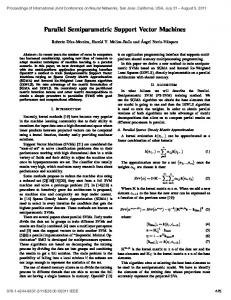
1. Introduction These proceedings discuss High Energy Physics (HEP) usage of Support Vector Machines (SVMs) [1], and in particular recent improvements to the functionality of the TMVA [2] implementation. These improvements are deployed in the ROOT git repository and from version 6.08. Having discussed this Machine Learning (ML) algorithm we proceed to raise the issue of generalisation of hyper-parameters (HPs); and in particular the use of hold-out and crossvalidation (CV). We also discuss the issues of understanding variance on the classification and performing a hypothesis test to address the issue of identifying if the HPs of a Multivariate Algorithm (MVA) are generalised, having used some method to promote HP generalisation. 2. SVMs SVMs were developed in the 1960’s in a hard margin form. These were based on Rosenblatt’s perceptron that allows one to trivially separate distinct types of data using a linear decision boundary, given by w · x + b [3]. Here w is a set of weights defining the orientation of the separating hyper-plane, b is the bias (offset from the origin) and x is an event. Subsequent developments expanded the power of SVMs in two significant ways; firstly to allow for misclassification of events and thereby extending the algorithm to a broader set of problems, including those encountered in a typical HEP analysis. This extension requires introduction of an overall cost parameter C for event mis-classification as well as slack parameters ξi for the mis-classification of any given event (or support vector, SV). Here C is a HP that alters the selection of the hyper-plane separating classes of event. This type of SVM is referred to as a Soft Margin SVM (see Fig 1). The second extension was to replace the use of scalar products between

two SVs, K(xi , xj ) = xi · xj , with inner products in terms of kernel functions (KFs) of SVs, K(xi , xj ) = hφ(xi ), φ(xj )i. These functions introduce additional HPs (KF parameters1 ) that need to be determined in order for one to separate classes of event. The use of KFs allows us to attempt to linearly separate types of event in a dual hyperspace of features F mapped implicitly from the input feature space X. It is not necessary to understand the mapping X 7→ F . For this mapping to exist a KF needs to be symmetric and satisfy Mercer’s condition [4]. For such kernels the algorithm can be used without detailed knowledge of the transformation; this is referred to as the kernel trick in the literature. While the kernel trick allows us to use complicated KFs it does obscure understanding of how the separating hyper-plane is determined. This plane is determined for a 1-norm SVM by optimising the dual space Lagrangian e L(α) =

n X

αi −

i=1

n 1X αi αj yi yj hxi · xj i , 2 i,j

(1)

to determine the Lagrange multipliers, αi ∈ [0, C], in order to maximise the margin. The Lagrange multipliersPare determined using Sequential Minimal Optimisation (SMO) and the constraint equation ni=1 αi yi = 0. Here the yi are example labels given by sign(hw · xi i + b). They denote which side of the decision boundary an event lies on. The functional margin of an example (xi , yi ) is given by γi = yi (hw · xi i + b) where positive values are obtained for correctly classified examples. The αi and SVs determine hyper-plane parameters as w and b are given by w =

n X

αi yi xi ,

(2)

i=1

maxyi =−1 (hw · xi i) + minyi =1 (hw · xi i) . (3) 2 SVMs are widely used outside of physics; for example in handwriting recognition, speech recognition, bioinformatics, risk analysis, finance, electronics, etc. Many of these problems involve distinguishing between features that are largely not overlapping; for example the classification of handwriting as illustrated by the MNIST classification example in TensorFlow [5]. Practitioners typically apply different KFs to a given problem in order to empirically validate that a given KF provides good performance for that problem. In doing so one implicitly relies on the kernel trick to work without trying to understand details of the problem in the dual feature space. The most commonly used KFs in HEP examples are scalar products and the radial basis function (RBF) where performance has been reported to be comparable with that for other ML algorithms; Neural Networks (NNs) and Boosted Decision Trees (BDTs). In contrast to other fields there has not been a broad uptake of SVMs within the HEP community. Several reports of SVMs use in HEP have been made: including jet flavour tagging and muon identification [6], top physics [7, 8], background suppression for W → eν signatures [9], and SUSY searches [10] at LEP, Tevatron and LHC experiments. Ref. [8] discusses a custom implementation of a SVM, and where specified the other references rely on the libsvm implementation [11]. A review of SVM use in HEP as of 2008 can be found in Ref. [12]. We have applied SVMs to Higgs physics [13], using the Kaggle Higgs Boson ML Challenge data sample [14]. The examples discussed below use the TMVA SVM algorithm implementation that uses SMO for Lagrange multiplier optimisation and Minuit [15] for hyper-parameter optimisation. b = −

2.1. Kernel Functions KFs used in previous HEP examples are scalar products and the RBF function. The latter is 2

K(xi , yi ) = e−Γ||xi −yi || , 1

Sometimes C is also referred to as a KF parameter.

(4)

x2

1 0.9 0.8 0.7

ξ i

0.6 0.5 0.4

w.

x+

0.3

b

0.2 0.1 0 0

0.1

0.2

0.3

0.4

0.5

0.6

0.7

0.8

0.9

1 x1

Figure 1. Soft margin SVM showing the (solid) maximal margin hyper-plane and (dashed) functional margins for two categories of events (dots and squares) in two dimensions.

where Γ = 1/2σ 2 is a HP to be optimised. Having just a single HP to determine (in addition to C) has the advantage of being a relatively cheap computing task. The disadvantage of the RBF function is that it assumes that the norm of the SV is sufficient to distinguish between events of different categories. Thus information may be lost in the computation of the KF for some problems. Computer Science literature discusses a number of other KFs, some of which we have added to TMVA. These include multi-Gaussian (MG) and polynomial (Poly) functions 

dim(x)

dim(x)

K(xi , yi ) =

Y

2

e−Γj (xij −yij ) , K(xi , yi ) = 

j=1

X

d

xij yij + c ,

(5)

j=1

respectively. The MG KF has dim(x) HPs, Γj , to overcome potential loss of information that the RBF may result in. The HPs of the Poly KF are c and d. The sum and product of KFs are also valid KFs and these four functions are now available in TMVA. 2.2. Hyper-parameter optimisation Logarithmic grid searches have been used (via libsvm and SVM-HINT) in order to determine HPs for RBF KFs. This is computationally inexpensive way to determine HPs for a KF with a low dimensionality, especially if it is of the form of an RBF or MG kernel. The error in selecting optimal HPs is governed by the granularity of the lattice used in the grid search. As soon as one moves to a high dimensionality of KF HPs this optimisation paradigm becomes expensive as the grid search scales with dim(x). To address this issue for TMVA the Davidon-Fletcher-Powell based Minuit optimisation algorithm [15] has been adopted for HP optimisation (HPO) 2 . HPO using this approach is more computationally expensive than the grid search approach for the 2D RBF optimisation problem however in general this provides a more accurate solution and is not specifically attuned to RBF and MG kernel functions, unlike the logarithmic grid search. 2.3. Other remarks Anecdotal remarks related to the use of SVMs note that these tend to result in a more generalised solution than other methods for a given sample size of training data. This is plausible and can be seen trivially for a hard margin SVM following the observation that the maximal margin hyper-plane is defined only by the SVs; hence only those, generally few, events on the decision boundary edges define the hyper-plane. It is not trivial to translate this observation to a soft 2

A grid search option is also being implemented for future release.

margin SVM, however in general a parallel situation will arise, where now it is the set of SVs with non-zero ξi that determine the definition of the decision boundary. The SVs with large values of ξi dominate the determination this boundary. In practice we observe better generalisation performance for SVMs with small training example sets compared with decision trees and neural networks in the comparisons that we have performed. While it is possible to optimise the HPs for a SVM, the issue of parameter generalisation remains one to be addressed as this is not guaranteed. Generalisation bounds exist for SVMs and methods used to promote generalised solutions are discussed further in Section 3. As mentioned above the hard margin SVM requires determination of the handful of SVs that fall on the functional margin to determine the HPs and hence decision boundary. Extending this to a soft margin SVM problem like those encountered with HEP background fighting problem the number of SVs routinely increases to encompass all training data. This means that the NSV × NSV Gramm matrix to be computed scales from a low dimensionality to a high dimensionality and becomes computationally expensive relative to training many other algorithms. This can be seen trivially by the computing time required to fit a SVM, vs that to train a NN or BDT using TMVA for a given data sample. Many of the SVs for a HEP soft margin problem have slack parameters that are small and therefore they do not significantly contribute to the determination of the maximal margin hyper-plane. The low ξi SVs are largely superfluous to the problem and a similar performance is attainable by presenting the SVM with a redacted data set that focuses on the SVs with ξi . In itself this observation is of little use as one needs to perform the SMO optimisation of the Lagrangian in order to determine the ξi ’s and in doing so therefore fix the Gramm matrix dimensionality accordingly. Data redaction or sparsification can be achieved by noting that the SVs with low value ξi ’s are far from the decision boundary. Hence if a-priori it is possible to identify regions far from the decision boundary then one can decrease compute cost by removing those regions from training at the expense of introducing an approximation to the definition of the maximal margin hyper-plane. 3. Generalisation Obtaining a set of hyper-parameters for an MVA that can provide predictive performance when applied to any unseen data sample consistent with the hyper-parameter optimisation is desirable. In HEP it is typical that generalisation is promoted using the hold-out technique (see below). HEP problems include both regression and classification variants. For classification we need to compare classification rates (or confusion matrices) and for regression problems we need to compare histograms to test for over-training. In practice a χ2 by eye or Kolomogrov-Smirnov (KS) test is performed on training and test histograms for the MVA output. In the case of TMVA the latter uses a binned implementation in the TH1 class that is known to be incorrect [16]. Furthermore the correctly calculated (un-binned) KS test statistic compares the similarity of the bulk of a distribution which is not the right comparison to make in general. This can be seen clearly for examples of searches for new particles in tails of distributions that corresponds to a large proportion of results in HEP at this time. The issue of similarity metrics is discussed elsewhere [17] and it is evident from that review that no single metric provides a general solution to this issue. We now consider three issues: firstly enhancing generalised behaviour at the HPO stage of algorithm tuning; secondly to determining if the set of HPs corresponds to generalised performance; thirdly to determine which MVA provides the best performance for a problem. Regarding the first point we focus on the hold-out (Section 3.1) and k-fold CV (Section 3.2) methods that are generally applicable to MVAs. Note that NNs use regularisation [18] and deep networks utilise dropout [19] and maxout [20] techniques. The second issue revolves around estimation of bias and variance for the ML algorithm and performing a hypothesis test to reject the null hypothesis that the HPs are generalised (Section 3.3) in order to choose an MVA model.

The third issue can be dealt with in a number of ways and in Ref. [21] we use a likelihood ratio test of a proxy of the observable being measured in order to illustrate this issue. 3.1. Hold-out method The “standard” method currently in use within HEP for promoting generalised HP determination for supervised learning algorithms is the hold-out CV method [22]. This involves dividing control (Monte Carlo simulated or real) data samples into two; taking one sample used for HPO (the training sample) and reserving the second sample to evaluate the performance of the HPs (the test sample). Some similarity test of the classification performance or binned distributions of the algorithm score can then be used to gauge if the HPs are generalised; however it is evident that this crucial step is sometimes overlooked. When this last step is not overlooked then often an incorrect binned KS test is performed as noted above 3 . Having performed the hold-out validation of HPs and assuming that the MVA passes a subsequent over-training check; the MVA is now ready to apply to unseen data (i.e. the physics analysis). Note that to apply an MVA to data used to determine HPs will result in a biased outcome and should be avoided. 3.2. Cross Validation The hold-out method suffers from the fact that half of the available training examples are used in order to determine the optimal HPs. This in turn can lead to a large variance in performance of the ML algorithm. One can improve upon hold-out by increasing the sample size used for HP training at the expense of the sample for validation. This introduces the issue of how to split the data into training and test samples as the optimal HPs obtained for a given training will depend on the data sampled from the available training examples as those examples reserved for validation are not used in HP determination. The k-fold CV algorithm divides the data sample into k distinct samples; and trains k sets of HPs using a training sample that reserves the k th sub-sample (or fold) for testing, the remaining k − 1 folds being used for training [23, 24]. This algorithm trains all permutations of leaving one fold out 4 . The fraction of training examples used for each permutation is (k − 1)/k. This results in a reduced variance for k > 2 compared with the hold-out approach as the k = 2 limit corresponds to that method. The the extreme limit where p (1) events are (is) reserved for testing is the leave p-out (one-out) CV method, for example see [25] and references therein. To avoid biases the training examples are independent of the test sample used to check HP generalisation prior to applying an MVA to unseen data. Having trained k sets of HPs the temptation is to select the best performing set according to some figure of merit (FOM), e.g. the receiver operating characteristic, ROC, integral at some pre-determined working point. This is a biased choice for the same reason that selecting the worst case scenario is also biased. It may lead to significant variation in MVA performance from one unseen data sample to the next. The aggregate performance of the ensemble of trainings corresponds to a more robust selection of HPs than the extremes, and the spread in performance obtained for the different trainings contains information about algorithm variance. Using the aggregate ensures that the error rate corresponds to the average error rate of the k folds; i.e. Pk E = i=1 Ei /k. A suitable number of folds k used for a particular problem needs to be determined on a case by case basis. We have introduced k-fold CV to TMVA. 3.3. Variance, Bias and testing for generalisation There are two relevant FOMs to optimise an algorithm on in particle physics, one is the precision of a measurement and the other is significance of a limit obtained from a search. However 3

To rely on the KS probability reported by the TH1 implementation to accept/reject a given training will lead to rejection of perfectly good trainings, which is to be avoided. 4 This is distinct from the bootstrap approach that would permit event oversampling.

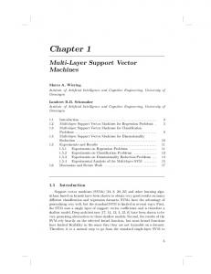
often these are not used as the metric when selecting MVAs as a considerable effort may be required to optimise an algorithm using one of these FOMs. Here we illustrate the situation encountered when optimising an MVA using significance as the appropriate FOM. We apply a stratified jackknife approach with 50 strata and construct samples of 2000 training and 2000 validation examples obtained using the MadGraph Monte Carlo simulation for a new particle search. Training and test samples are statistically independent and each training sample is used to train a boosted decision tree (BDT) to distinguish between one signal and one background class of events. To force overfitting we train BDTs with a depth between 2 and 10 (labeled as samples 0 through 8, respectively). Figure 2 shows black (red) points representing the average significance obtained for the training (test) samples. The band illustrated for the black points is an estimate of the standard deviation applied to the test sample. The difference between red and black points indicates the level of HP overtraining as tree depth increases.

Figure 2. Illustrating overtraining with increasing tree depth for the example in the text.

If the end result of a measurement is not used to construct the FOM to check for generalisation then we can consider performing a hypothesis test on the MVA output; either confusion matrices (for classification) or sets of histograms (for regression). The null and alternate hypotheses, H0 and H1 , respectively are H0 : the MVA is generalised and H1 : the MVA is not generalised for all classes of event. For a classification problem with 2 species of event the fraction of (in)correctly classified species of events is indicated in the 2 × 2 confusion matrix that describe the binomial classification of event type. The parent distribution is estimated using the average of the train and test confusion matrices. It straight forward to construct a hypothesis test that can be used to assert if H0 is generalised at a given confidence level 1 − α. For more than 2 species of event this approach can be extended to the corresponding multinomial problem. For a regression analysis, instead of a confusion matrix we have a pair of histograms (one for test and one for train samples) for each species of event. We can construct an estimator of the underlying distributions to perform a hypothesis test in analogy with a classification problem, where now we use a multinomial estimator for the fraction of events expected in each bin. 3.4. Example: H → τ + τ − To illustrate the ML issues discussed above we now turn to a concrete HEP example, the search for H → τ + τ − at the LHC. This decay has one τ decaying leptonically and the other decaying hadronically, and the final state is not fully reconstructed due to the undetected neutrinos. This is not a fully optimised study, but rather an illustration of potential using a limited set of input features from the Kaggle data set. We use the following input features: the estimated Higgs mass using the missing mass calculator MMC, transverse mass of the missing energy and lepton

mT (ETmiss , `), the R separation between the hadronically and leptonically reconstructed τ ’s ∆R(τ, `), ratio of transverse momenta for the leptonic and hadronic τ ’s p`T /pτT , φ Centrality, and missing transverse energy ETmiss . Distributions of input features for the signal and background are shown in Figure 3. This highlights that the data are overlapping and the signal features are always found in regions of space that are also occupied by background in X. These high level derived features are input to SVMs with the RBF, MG, and Poly KFs and to a BDT for performance comparison. All trainings use the hold-out approach and the corresponding ROC curves are shown in Figure 4. One can see that the SVMs are able to give similar performance to the BDTs in this example; a result consistent with the conclusions of previous studies with SVM in HEP. We also note that there is some variation in performance depending on choice of KF for this problem with the MG KF performing the worst.

400

0.01 0.005 0

500

50

100

mmc

0.6 0.5 0.4 0.3 0.2 0.1 2

3

4

5

6

7

(1/N) dN / 0.0725

U/O-flow (S,B): (0.0, 0.0)% / (0.0, 0.1)%

(1/N) dN / 0.207

0.8 0.7

0.6 0.5 0.4 0.3 0.2 0.1 0

250

1

2

3

3.5 3 2.5 2 1.5 1 0.5 0

8

−1

−0.5

0

5

Input variable: PRI_met_sumet

4

DER_pt_ratio_lep_tau

4

deltar_tau_lep

Input variable: DER_met_phi_centrality

0.9

1

200

0.7

mass_transverse_met_lep

Input variable: DER_pt_ratio_lep_tau

0

150

0.8

U/O-flow (S,B): (0.0, 0.0)% / (0.0, 0.0)%

U/O-flow (S,B): (0.0, 0.0)% / (0.0, 0.0)%

0.015

0.9

0.5

1

0.005 U/O-flow (S,B): (0.0, 0.0)% / (0.0, 0.0)%

300

0.02

(1/N) dN / 28.2

200

0.025

U/O-flow (S,B): (0.0, 0.0)% / (0.0, 0.0)%

100

Input variable: deltar_tau_lep

(1/N) dN / 0.133

Input variable: mass_transverse_met_lep

Signal Background

(1/N) dN / 6.3

0.024 0.022 0.02 0.018 0.016 0.014 0.012 0.01 0.008 0.006 0.004 0.002 0

U/O-flow (S,B): (0.0, 0.0)% / (0.0, 0.3)%

(1/N) dN / 13.3

Input variable: mmc

0.004 0.003 0.002 0.001 0

200

400

600

DER_met_phi_centrality

800

1000

PRI_met_sumet

Figure 3. Distributions of input features for signal and background for the H → τ + τ − .

ROC-Curve SVM_Holdout_RBF

0.9

SVM_Holdout_Poly SVM_Holdout_MG

0.8

BDT_Holdout

0.7 0.6

Backgr rejection (1-eff)

Backgr rejection (1-eff)

ROC Curves

SVM_Best

0.9

0.6 0.5

0.4

0.4

0.3

0.3

0.2

0.2 0.5

0.6

0.7

0.8

0.9

1 Signal eff

SVM_Holdout_RBF

0.7

0.5

0.1 0.4

SVM_Average

0.8

0.4

0.5

0.6

0.7

0.8

0.9

1 Signal eff

Figure 4. ROC curves for SVMs and a BDT as discussed in the text using (left) hold-out and (right) with 5-fold CV. The best and average SVMs determined in the CV process are shown to illustrate the variation between these two. We proceed to explore application of k-fold CV to this problem. The number of folds to use needs to be determined anecdotal for a given problem. Here we illustrate the effect of CV on

ROC integral in comparison with the hold-out technique for a 5-fold CV (see Fig. 4). The best and average ROC curves are found to be similar; and while it is tempting to take the training corresponding to the best ROC integral to derive the nominal HP set, that is not guaranteed to provide a typical performance for the algorithm when presented with unseen data. The average solution corresponds to a more robust HP choice for application of the algorithm to unseen data. As mentioned above the CV method is not specific to SVMs and can be applied to other MVAs such as NNs and BDTs. TMVA has been extended to include a CV tool based on this work. Having promoted generalisation using CV one still has to address the question of HP fine tuning as these methods do not guarantee that the optimised HP set determined correspond to a generalised result. Likewise when using more than one MVA, the ROC curve is not sufficient to determine which MVA leads to the best result. For that one has to apply the MVA to an analysis and follow through to the end result, or some proxy thereof; for example some FOM relating to significance such as the approximate mean significance used in Ref. [13]. 4. Summary We have discussed the use of SVMs in the context of HEP. Here we focus on the example of searching for the H → τ + τ − mode at the LHC in the context of functionality available in TMVA. We also discuss the issue of generalisation, highlighting some pitfalls in current practice as well as issues to be considered when determining HPs for a given ML algorithm. While CV is an improvement over the hold-out method, this does not guarantee generalisation. Thus one should establish if an MVA is generalised having previously attempted to improve the robustness of HP determination via CV or some other method. The issues of how to illustrate overtraining by using jackknife event selection and by hypothesis testing have been discussed. References [1] [2] [3] [4] [5]

C. Cortes and V. Vapnik, Machine Learning 20 Issue 3 (1995). A. Hoecker et al., PoS ACAT 040 (2007) 040. F. Rosenblatt, Psychol. Rev. 65, 386-408 (1958). J. Mercer, Philo. Trans. Roy. Soc. London, A 209:415-446 (1909). Y. LeCun et al., Proceedings of the IEEE, 86(11):2278-2324, November 1998. Also see http://yann.lecun.com/exdb/mnist/ and https://www.tensorflow.org. [6] P. Vannerem, K. R. Muller, B. Scholkopf, A. Smola and S. Soldner-Rembold, hep-ex/9905027. [7] A. Vaiciulis, Nucl. Instrum. Meth. A 502 (2003) 492. [8] B. E. Whitehouse, FERMILAB-THESIS-2010-61. [9] F. Sforza and V. Lippi, Nucl. Instrum. Meth. A 722 (2013) 11. ¨ Sahin, D. Krcker and I. A. Melzer-Pellmann, Nucl. Instrum. Meth. A 838 (2016) 137. [10] M. O. [11] C.-C. Chang and C.-J. Lin, LIBSVM: A library for support vector machines, ACM Transactions on Intelligent Systems and Technology, 2 2011 27:1–27:27. [12] A. Vossen, arXiv:0803.2345 [physics.data-an]. [13] C. Adam-Bourdarios, G. Cowan, C. Germain-Renaud, I. Guyon, B. Kgl and D. Rousseau, J. Phys. Conf. Ser. 664 (2015) No.7, 072015. See also URL: http://higgsml.lal.in2p3.fr/documentation/ (2014). [14] A. Bethani, A. J. Bevan, J. Hays and T. J. Stevenson, arXiv:1610.09932 [physics.data-an]. [15] F. James and M. Winkler, “MINUIT User’s Guide; F. James, CERN-D-506, CERN-D506. [16] See the TH1::KolmogorovTest function implementation https://root.cern.ch/doc/master/classTH1.html [17] S.-H. Cha, Int. J. Math. Models and Methods in Applied Sciences, 1 300-307 (2007); F. C. Porter, arXiv:0804.0380 [physics.data-an]. [18] For example see C. M. Bishop, Neural Networks for Pattern Recognition, Clarendon Press (1996). [19] G. E. Hinton et al. CoRR, abs/1207.0580 (2012). [20] I. J. Goodfellow, D. Warde-Farley, M. Mirza, A. Courvill, Y. Bengio, JMLR WCP 28 (3): 1319-1327 (2013). [21] J. Hays, A. Bevan, T. J. Stevenson, proceedings of ICHEP 2016 (to appear in PoS). [22] L. Devroye and T. J. Wagner, IEEE Transaction in Information Theory, 25 (5):601604 (1979). [23] M. Stone, J. Roy. Statist. Soc. Ser. B, 36 111147 (1974). [24] S. Geisser, J. Amer. Statist. Assoc., 70:320328 (1975). [25] S. Arlot, Stat. Surveys 4 (2010) 4079.