Support Vector Machines Approach to Credit

Support Vector Machines Approach to Credit Assessment∗ Jianping Li 1,2, Jingli Liu1,2, Weixuan Xu2 and Yong Shi3 1

3

University of Science & Technology of China, Hefei, 230026, P.R.China 2 Institute of Policy and Management, Chinese Academy of Sciences, Beijing 100080, P.R.China [email protected], [email protected]

Graduate School of Chinese Academy of Sciences, Beijing 100039, P.R.China [email protected]

Abstract. Credit assessment has attracted lots of researchers in financial and banking industry. Recent studies have shown that Artificial Intelligence (AI) methods are competitive to statistical methods for credit assessment. This article applies support vector machines (SVM), a relatively new machine learning technique, to the credit assessment problem for better explanatory power. The structure of SVM has many computation advantages, such as special direction at a finite sample and irrelevance between the complexity of algorithm and the sample dimension. A real credit card data experiment shows that SVM method has outstanding assessment ability. Compared with the method that is currently used by a major Chinese bank, the SVM method has a great potential superiority in predicting accuracy. Key words: Credit assessment; Classification; Support vector machines

1. Introduction Credit risk management has played a key role in financial and banking industry. Inferior credit risk assessment tool is the primary reason of enterprise bankruptcy. Generally speaking, credit risk management includes credit risk analysis, assessment (measurement) of enterprise credit risk and how to manage the risk efficiently, while credit risk assessment is the basic and critical factor in credit risk management. The main purpose of credit risk assessment is to measure the default possibility of borrowers and provide the loaner a decision-aid by conducting qualitative analysis and qualitative computation to the possible factors that will cause credit risk. At present, the classification is the most popular method used in credit risk assessment. That is, according to the financial status of the borrowers, we can use a credit scoring system to estimate the corresponding risk rate so that the status can be classified as ∗

This research has been partially supported by National Excellent Youth Fund under 70028101, and the President Fund of Chinese Academy of Sciences (CAS) (2003).

normal or default. Thus the problem can be transformed to some kind of classification. The Multivariate Statistical Analysis technique especially Multiple Discriminant Analysis (MDA) has been widely used in credit risk classification. This basic idea is to use the historical sample as training set to build a discriminant function and use the function to classify the new sample. The outstanding advantage of Multivariate Statistical Analysis is that it is simple and easy to interpret. But the requiring of multiple normal distributed data and the equality of covariance matrix is conflict with the real data. Thus it brings many questions [1]. In order to solve this problem, researchers modified MDA from different aspects, for example, adopting logarithmic transformation, QDA model, Logit analysis model, neural network model and decision tree [2, 3]. These techniques can partially solve the problem, but they are not perfect. In general, the modification of MDA is not ideal. Because of the complexity of credit risk and various data structure, the theoretical advantage of many methods doesn’t work well in practice. In China’s situation, lacking of samples and high dimension are the notable characters of Chinese credit data. Because the historical sample data is small and the data character used in credit risk classification is not steady, using MDA in credit risk classification will not produce practical results [4]. This paper applies Support Vector Machine (SVM) to the field of credit assessment. SVM is a novel learning machine based on mathematical programming theory, which has yielded excellent performance on a wide range of problems. The remainder of the paper is structured as follows. The basic principle of SVM follows first the introduction. Then, some ideas how to use SVM in credit risk management is provided. In the experimental study, we provide descriptions of the data sets, the experiment results and analysis. We also conduct a comparison study to the current method used in a major Chinese commercial bank. Finally, we discuss the future research directions.

2. Analytical methods 2.1 Review of support vector machines Since the mid of 1990, SVM appeared with the continuous development and maturation of machine learning theory. It has exhibited performance which superior to the other existing methods. SVM is a novel learning machine introduced first by Vapnik [5]. It is a theory of machine learning focusing on small sample data based on the structural risk minimization principle from computational learning theory. Hearst et al. [6] positioned the SVM algorithm at the intersection of learning theory and practice: ‘‘it contains a large class of neural nets, radial basis function (RBF) nets, and polynomial classifiers as special cases. Yet it is simple enough to be analyzed mathematically, because it can be shown to correspond to a linear method in a high dimensional feature space nonlinearly related to input space.’’ In this sense, support vector machines can be a good candidate for combining the strengths of more theory-driven

and easy to be analyzed conventional statistical methods and more data-driven, distribution free and robust machine learning methods. The main advantages of SVM can be summarized as follows: 1) SVM is used in the situation of finite sample data. It aims to get the optimal solution based on the present information rather than the optimal value when the number of sample tends to be infinite. 2) The algorithm is finally transformed into the optimization of quadratic program. Theoretically, it will get a global optimization value, which solves the unavoidable local optimization problem while using neural network. 3) The algorithm performs a nonlinear mapping from the original data space into some high dimension feature space, in which it constructs a linear discriminant function to replace the nonlinear functions in the original data space. This special character assures that SVM has good generalization ability. At the same time, it solves the problem of dimension disaster because its computation complexity is independent to the sample dimension. A brief description of the SVM algorithm is provided here, for more details please refer to Refs [7, 8]. Consider the problem of separating the set of training vectors belonging to two separate 1

1

l

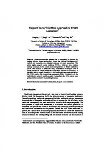
classes. D= {(x , y ),…, (x , y )}, x ∈ R , y ∈ {-1,1}, with a hyper plane, (ω ⋅ x ) + b = 0. Figure 1 is a simple linearly separatable case. Solid points and circle points represent two kinds of sample separately. H is the separating line. H 1 and H 2 are the closest lines parallel to the separating line of Fig. 1. Optimal Separating Hyperplane the two-class sample vectors. The distance between H 1 and H 2 is called margin. The separating hyperplane is said to be optimal if it classifies the samples into two classes without error (training error is zero) and the margin is maximal. The sample vectors in H 1 , H 2 are called support vectors. The separating l

n

hyperplane equation is (ω ⋅ x ) + b = 0, where the sample vectors (x i , y i ), i=1,…, n, should satisfy

y i [ (ω ⋅ x ) + b] ≥ 1, i =1,…, n.

The distance of point x to the hyperplane ( ω , b) is d (ω , b; x ) =

(2.1) (ω ⋅ x ) + b I

ω

. The

optimal hyperplane is given by maximizing the margin d , subject to equation (2.1).

The margin can be given by

ρ (ω , b) =

2

ω

. Hence the hyperplane that optimally

separates the data is the one that minimizes ω

φ (ω ) =

(2.2)

2

The Lagrange function of (2.2) under constraints (2.1) is,

φ (ω , b, a ) =

1 2

l

ω － ∑α i ( y i [(ω , x i ) + b] − 1) , 2

(2.3)

i =1

The optimal classification function, if solved, is f (x ) = sgn (ω ⋅ x) + b ). For nonlinear case, we map the original space into a high dimension space by a nonlinear mapping, in which an optimal hyperplane can be sought. The inner product function enables the classification in the new space, however, the computation complexity will not increase. Thus the corresponding program is, ∗

n

Q(α ) = ∑ α i − i =1

∗

1 n ∑ α iα j y i y j K (x i , x j ) * 2 i , j =1

(2.4)

The corresponding separating function is, n

f ( x ) = sgn( ∑ α i* yi K ( xi , x ) + b* )

(2.5)

i =1

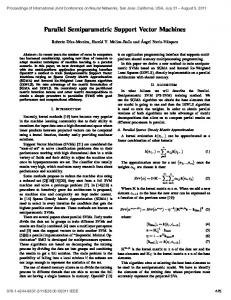
This is the so- called SVM. SVM provides a method to solve the possible dimension disaster in the algorithm: when constructing a discriminant function, SVM does not obtain solution in the feature space after mapping the original sample space into a high dimension space by nonlinear mapping. Instead, it compares the sample vectors (for example, computes sample vectors’ inner product or some kinds of distance) in the input space, then it performs nonlinear mapping after the comparison [9]. Thus, most of the work will be carried out in the input space instead of the high dimension feature space. The separating function of SVM is like a neural network. The output is the linear combination of middle nodes and each middle node corresponds to a support vector. See figure 2 below:

y

Output (decision rule)： s

α1 y1

α2 y 2

K ( x2 , x)

K ( x1 , x)

y = sgn( ∑ α i y i K ( x i , x ) + b i =1

αs y s

Weight

α i yi

K ( xs , x )

Nonlinear mapping based on support vectors (inner product) Input

x1

x2

d

x

Fig. 2. An Illustration of Support Vector Machine

vectors

x = ( x , x ,..., x ) 1

2

d

Function K is called the kernel function of dot product. In [10], it is defined as a distance between sample vectors. The method above can assure all training samples are accurately classified. That is, on condition that the empirical risk is zero, SVM can get the best generalization ability by maximizing the margin. However, different kinds of dot product in SVM can accomplish such works as Polynomial approaching, Bayesian classifier, and Radial Basic Function. How to define the dot product is critical to the classification result. With these advantages of SVM, we attempt to apply SVM to the credit risk management because the feature of credit database can be potentially attacked by SVM. 2.2 Applications in credit assessment In the last few years, there have been substantial developments in different aspects of support vector machine. These aspects include theoretical understanding, algorithmic strategies for implementation and real-life applications. SVM has yielded high performance on a wide range of problems including pattern recognition [10, 11, 12], function approach [13], data mining [14] and nonlinear system control [15] etc. These application domains typically have involved high-dimensional input space, and the performance is also related to the fact that SVM’s learning ability can be independent of the dimensionality of the feature space. The SVM approach has been applied in several financial applications recently, mainly in the area of time series prediction and classification [16, 17]. A recent study closely related to our work investigated the use of the SVM approach to predict credit rating analysis with a market comparative study. They reported that SVM achieved accuracy comparable to that of back-propagation neural networks [18]. In this study, we are interested in evaluating the performance of the SVM approach in credit assessment in comparison with that of the method currently being used by a major Chinese commercial bank. The standard SVM formulation solves only the binary classification problem. While in credit risk assessment, it is not enough to classify the evaluation object into two classes. Hsu and Lin’s recent paper [19] compared several methods for multi-class SVM and concluded that ‘one-against-one’ and DAG are more suitable for practical uses. This result offers a good solution to method selection in credit risk assessment. In practical application, we use a sample consists of n variables to assess the personal credit risk, for each variable value of training sample, we want to find an interpretive vector x i ∈ R d and a symbol y i that describes which class the indicator value belongs to. Then we predict new sample classification after training.

3. Experiment results and analysis 3.1 Data sets We have used real life credit card data to conduct the experiment. We selected one thousand sample data from a Chinese commercial bank, of which two classes have been defined: good and bad credit. We separate the credit applicants into two classes: good and bad. There are 245 bad records and 755 good records in the total sample. 14 variables are selected for personal credit assessment. The variables are listed in table 1. Table 1. The assessment variables

Index 1 2 3 4 5 6 7 8 9 10 11 12 13 14

Indicators Year of birth Number of children Number of other dependents Is there a home phone Spouse's income Applicant's employment status Applicant's income Residential status Value of Home Mortgage balance outstanding Outgoings on mortgage or rent Outgoings on Loans Outgoings on Hire Purchase Outgoings on credit cards

3.2 Experiment results and analysis We use Matlab6.1 and Osusvms3.00 toolbox developed by Junshui Ma, Yi Zhao and Stanley Ahalt [20] to conduct the computation. We divide the total sample into two parts: one is used for training and the other for test. Table 2 lists the predicting accuracy results of different number of training sample.

Table 2. Predicting accuracy

The ratio of training set to total sample 10% 20% 25% 33.33% 50% 66.67% 75% 90%

Predicting Predicting accuracy of accuracy of test training sample sample 0.9098 0.7153 0.9430 0.7102 0.9085 0.7095 0.9093 0.7062 0.8873 0.6900 0.8873 0.6455 0.8715 0.6352 0.8648 0.6098

Mean Predicting accuracy 0.8125 0.8266 0.8090 0.8077 0.7886 0.7664 0.7533 0.7373

The result shows that the mean predicting accuracy is all above 70%. If we use less than 1/3 of the total sample as training sample and the rest as test sample, the results will be better, where the predicting accuracy will be above 80%. The preliminary result indicates that the application of SVM can improve the classification accuracy. However, we observe that the result of the predicting accuracy on training sample is better than that of test sample, which shows the predicting ability is not very good and needs further study.

4. A comparison result In order to further verify the practical effect, we conducted a comparative study. We compare the SVM method with the basic grade criterion (mainly used for the grant of credit card to applicants) which is presently used by the Chinese bank for personal credit bound. The indicators used in that method is almost the same as those in SVM. We use that criterion to get a grade for each sample, by which to classify the sample into two classes: good and bad. An applicant would get credit if his/her grade is no less than the threshold value determined by the bank (in this criterion the lowest grade is 110). The results are listed in table 3: Table 3. the predicting accuracy of the present method used by a Chinese bank

Total number 1000

False classification Correct classification number number 449

551

Accuracy 55.1%

The predicting accuracy of current method is 55.1%. Compared with the result outlined in table 2, this accuracy is much lower than that of SVM. The predicting accuracy of SVM can exceed current method result by 50%. This can illustrate that

the assessment classification result got by using SVM has obvious superior to the current method of the bank. At the same time, the accuracy of 55.1% shows that the current method of the bank has big problem in credit card risk management and needs to be improved urgently. Further discussion about this situation can be referred to [21].

5. Conclusion and future research This paper has applied the SVM approach to credit assessment and reported a comparison study with the current credit assessing method of a major Chinese commercial bank. The preliminary experiment results show that the SVM method turns out to be an effective classification tool for credit assessment. The comparison analysis indicates the SVM method is better than the current method of the Chinese commercial bank, which the predicting accuracy can increase 50%. Our future directions of the research would focus on how to improve the predicting accuracy especially in the testing sample and compare the SVM method with other well-known methods, such as the back-propagation neural networks and decision tree. Inspired by the preliminary results, we believe that deeper data processing and more suitable kernel function selection will contribute to increase the predicting accuracy. Extending the two-class classification to multi-class classification is also our future research work.

Reference 1. 2. 3. 4. 5. 6. 7. 8. 9. 10.

Eisenbeis R A., Pitfalls in the application discriminant analysis in business and economics. Journal of Finance, (1977) 32: 875-900. Tam K Y, Kiang M. Managerial applications of neural networks: the case of bank failure predictions. Management Sciences, (1992) 38(1): 926- 947. Frydm an H, Altman E I, Kao Duen Li. Introducing recursive partitioning for financial classification: the case of financial distress. Journal of Finance, (1985) 40 (1): 269-291. Chunfeng Wang, Research on small sample data credit risk assessment. Journal of Management Science in China, (2001)4(1): 28-32 (in Chinese). V.Vapnik. Nature of Statistical Learning Theory. New York, Springer-Verlag,. (1995) M.A Hearst, S.T. Dumais, E.Osman, J. Platt, B.Scholkopf. Support Vector Machines, IEEE Intelligent System, (1998)13(4):18-28 N. Cristianini, J. Shawe-Taylor, An Introduction to Support Vector Machines, Cambridge Univ. Press, Cambridge, NewYork (2000). K.-R. Mu¨ller, S. Mika, etc. An introduction to kernel-based learning algorithms, IEEE Transactions on Neural Networks(2001) 12 (2) , 181– 201. Corinna Cortes, V.Vapnik. Support-Vector Network. Machine Learning, (1995) 20.273-297 J.C.Burges. A Tutorial on Support Vector Machines for Pattern Recognition. Bell Laboratories, Lucent Technologies(1997).

11.

12. 13. 14.

15. 16. 17.

18. 19. 20. 21.

Roobacert D. Hulle M M Van. View-based 3d Object Recognition with Support Vector Machines: an Application to 3d Object Recognition with Cluttered Background. In Proc. SVM Workshop at IJCAI’99, Stockholm, Sweden(1999) Scholkopf B, et al. Face Pose Discrinination Using Support Vector Machines, in: Proceedings of CVPR 2000, Hilton Head Island, (2000)430-437. Sola A J, Scholkopf B. A Tutorial on Support Vector Regression [J], NeuorCOLT TR NC-TR-98-030, Royal Holloway College, University of London, UK. (1998) Bradley P. Mathematical Programming Approaches to Machine Learning and Data Mining. Ph.D thesis. University of Wisconsin, Computer Science Department, Madison, WI, USA, TR-98-11 (1998). Suykens J A K, et al. Optimal Control by Least Squares Support Vector Machines. Neural Networks, (2001)14(1): 23-25 F.E.H. Tay, L.J. Cao, Modified support vector machines in financial time series forecasting, Neurocomputing, (2002)48: 847– 861. T. Van Gestel, J.A.K. Suykens, etc, Financial time series prediction using least squares support vector machines within the evidence framework, IEEE Transactions on Neural Networks, (2001)12 (4):809– 821. Zan Huanga, Hsinchun Chen, etc. Credit rating analysis with support vector machines and neural networks: a market comparative study. Decision Support Systems (In press). C.W.Hsu, C.J.Lin. A Comparison of Methods for Multi-class Support Vector Machines, Technical Report, National Taiwan University, Taiwan (2001). http://www.csie.ntu.edu.tw/~cjlin/libsvm/index.html Jianping Li, Jingli Liu, etc. An improved credit scoring method for Chinese commercial banks. working paper (2004).