error of a model, rather than minimizing the Mean Square Error over the data set (as Empirical Risk Minimization methods do), training a SVM to obtain the ...
MASSACHUSETTS INSTITUTE OF TECHNOLOGY ARTIFICIAL INTELLIGENCE LABORATORY and
CENTER FOR BIOLOGICAL AND COMPUTATIONAL LEARNING DEPARTMENT OF BRAIN AND COGNITIVE SCIENCES A.I. Memo No. 1602 C.B.C.L Paper No. 144
March, 1997
Support Vector Machines: Training and Applications Edgar E. Osuna, Robert Freund and Federico Girosi
This publication can be retrieved by anonymous ftp to publications.ai.mit.edu. The pathname for this publication is: ai-publications/1500-1999/AIM-1602.ps.Z
Abstract The Support Vector Machine (SVM) is a new and very promising classi�cation technique developed by Vapnik and his group at AT&T Bell Laboratories �3, 6, 8, 24]. This new learning algorithm can be seen as an alternative training technique for Polynomial, Radial Basis Function and Multi-Layer Perceptron classi�ers. The main idea behind the technique is to separate the classes with a surface that maximizes the margin between them. An interesting property of this approach is that it is an approximate implementation of the Structural Risk Minimization (SRM) induction principle �23]. The derivation of Support Vector Machines, its relationship with SRM, and its geometrical insight, are discussed in this paper. Since Structural Risk Minimization is an inductive principle that aims at minimizing a bound on the generalization error of a model, rather than minimizing the Mean Square Error over the data set (as Empirical Risk Minimization methods do), training a SVM to obtain the maximum margin classi�er requires a di�erent objective function. This objective function is then optimized by solving a large-scale quadratic programming problem with linear and box constraints. The problem is considered challenging, because the quadratic form is completely dense, so the memory needed to store the problem grows with the square of the number of data points. Therefore, training problems arising in some real applications with large data sets are impossible to load into memory, and cannot be solved using standard non-linear constrained optimization algorithms. We present a decomposition algorithm that can be used to train SVM's over large data sets. The main idea behind the decomposition is the iterative solution of sub-problems and the evaluation of, and also establish the stopping criteria for the algorithm. We present previous approaches, as well as results and important details of our implementation of the algorithm using a second-order variant of the Reduced Gradient Method as the solver of the sub-problems. As an application of SVM's, we present preliminary results in Frontal Human Face Detection in images. This application opens many interesting questions and future research opportunities, both in the context of faster and better optimization algorithms, and in the use of SVM's in other pattern classi�cation, recognition, and detection applications. Copyright c Massachusetts Institute of Technology, 1996 This report describes research done within the Center for Biological and Computational Learning in the Department of Brain and Cognitive Sciences and the Arti�cial Intelligence Laboratory at the Massachusetts Institute of Technology. This research is sponsored by MURI grant N00014-95-1-0600� by a grant from ONR/ARPA under contract N00014-92-J-1879 and by the National Science Foundation under contract ASC-9217041 (this award includes funds from ARPA provided under the HPCC program). Edgar Osuna was supported by Fundaci�on Gran Mariscal de Ayacucho and Daimler Benz. Additional support is provided by Daimler-Benz, Eastman Kodak Company, Siemens Corporate Research, Inc. and AT&T.
Contents 1 Introduction 2 Support Vector Machines
2.1 Empirical Risk Minimization : : : : : : : : : : : : : : : : : : : : : 2.2 Structural Risk Minimization : : : : : : : : : : : : : : : : : : : : : 2.3 Support Vector Machines: Mathematical Derivation : : : : : : : : 2.3.1 Linear Classi er and Linearly Separable Problem : : : : : : 2.3.2 The Soft Margin Hyperplane: Linearly Non-Separable Case 2.3.3 Nonlinear Decision Surfaces : : : : : : : : : : : : : : : : : : 2.4 Additional Geometrical Interpretation : : : : : : : : : : : : : : : : 2.5 An Interesting Extension: A Weighted SVM : : : : : : : : : : : : :
3 Training a Support Vector Machine
3.1 Previous Work : : : : : : : : : : : : : : : : : : : : 3.1.1 Methods Description : : : : : : : : : : : : : 3.1.2 Computational Results : : : : : : : : : : : : 3.2 A New Approach to Large Database Training : : : 3.2.1 Optimality Conditions : : : : : : : : : : : : 3.2.2 Strategy for Improvement : : : : : : : : : : 3.2.3 The Decomposition Algorithm : : : : : : : 3.2.4 Computational Implementation and Results 3.3 Improving the Training of SVM: Future Directions
4 SVM Application: Face Detection in Images
: : : : : : : : :
: : : : : : : : :
: : : : : : : : :
: : : : : : : : :
: : : : : : : : :
4.1 Previous Systems : : : : : : : : : : : : : : : : : : : : : : : : 4.2 The SVM Face Detection System : : : : : : : : : : : : : : : 4.2.1 Experimental Results : : : : : : : : : : : : : : : : : 4.3 Future Directions in Face Detection and SVM Applications
5 Conclusions
: : : : : : : : : : : : :
: : : : : : : : : : : : :
: : : : : : : : : : : : :
: : : : : : : : : : : : :
2 2
: : : : : : : :
: : : : : : : :
: : : : : : : :
: : : : : : : :
: : : : : : : :
: : : : : : : :
: : : : : : : :
: : : : : : : :
: : : : : : : :
: : : : : : : :
: : : : : : : :
: : : : : : : :
: : : : : : : :
: 2 : 4 : 4 : 4 : 8 : 10 : 14 : 14
: : : : : : : : :
: : : : : : : : :
: : : : : : : : :
: : : : : : : : :
: : : : : : : : :
: : : : : : : : :
: : : : : : : : :
: : : : : : : : :
: : : : : : : : :
: : : : : : : : :
: : : : : : : : :
: : : : : : : : :
: : : : : : : : :
: : : : : : : : :
: : : :
: : : :
: : : :
: : : :
: : : :
: : : :
: : : :
: : : :
: : : :
: : : :
: : : :
: : : :
: : : :
: : : :
15
16 16 20 20 21 23 24 24 25
28
29 29 30 30
31
1
1 Introduction In this report we address the problem of implementing a new pattern classi cation technique recently developed by Vladimir Vapnik and his team at AT&T Bell Laboratories �3, 6, 8, 24] and known as Support Vector Machine (SVM). SVM can be thought as an alternative training technique for Polynomial, Radial Basis Function and Multi-Layer Perceptron classi ers, in which the weights of the network are found by solving a Quadratic Programming (QP) problem with linear inequality and equality constraints, rather than by solving a non-convex, unconstrained minimization problem, as in standard neural network training techniques. Since the number of variables in the QP problem is equal to the number of data points, when the data set is large this optimization problem becomes very challenging, because the quadratic form is completely dense and the memory requirements grow with the square of the number of data points. We present a decomposition algorithm that guarantees global optimality, and can be used to train SVM's over very large data sets (say 50,000 data points). The main idea behind the decomposition is the iterative solution of sub-problems and the evaluation of optimality conditions which are used both to generate improved iterative values, and also establish the stopping criteria for the algorithm. We demonstrate the e�ectiveness of our approach applying SVM to the problem of detecting frontal faces in images, which involves the solution of a pattern classi cation problem (face versus non-face patterns) with a large data base (50,000 examples). The reason for the choice of the face detection problem as an application of SVM is twofold: 1) the problem has many important practical applications, and received a lot of attention in recent years� 2) the di�culty in the implementation of SVM arises only when the data base is large, say larger than 2,000, and this problems does involve a large data base. The paper is therefore divided in two main parts. In the rst part, consisting of sections 2 and 3 we describe the SVM approach to pattern classi cation and our solution of the corresponding QP problem in the case of large data bases. In the second part (section 4) we describe a face detection system, in which the SVM is one of the main components. In particular, section 2 reviews the theory and derivation of SVM's, together with some extensions and geometrical interpretations. Section 3 starts by reviewing the work done by Vapnik et al. �5] in solving the training problem for the SVM. Section 3.1.1 gives a brief description and references of the initial approaches we took in order to solve this problem. Section 3.2 contains the main result of this paper, since it presents the new approach that we have developed to solve Large Database Training problems of Support Vector Machines. Section 4 presents a Frontal Human Face Detection System that we have developed as an application of SVM's to computer vision object detection problems.
2 Support Vector Machines In this section we introduce the SVM classi cation technique, and show how it leads to the formulation of a QP programming problem in a number of variables that is equal to the number of data points. We will start by reviewing the classical Empirical Risk Minimization approach, and showing how it naturally leads, through the theory of VC bounds, to the idea of Structural Risk Minimization (SRM), which is a better induction principle, and how SRM is implemented by SVM.
2.1 Empirical Risk Minimization
In the case of two-class pattern recognition, the task of learning from examples can be formulated in the following way: given a set of decision functions ff (x) : � 2 �g�
f : 0( d^i ) if d^ 6� 0 1 if d � 0
with b^ = b2 ; A2 xk and d^ = A2 dk . 5. Let xk+1 = xk + k dk . Let k = k + 1. Go to step 2. Step 2 involves solving a linear program, which is usually very easy to .In the case of training a SVM, step 2 becomes: Maximize subject to
f (d) = (1 ; D k ) � d
�d ;1 � di 0 � di ;1 � di
=0 �0 �1 �1
(48)
for �i = C for �i = 0 otherwise
and step 4 selects k = min( opt � max), where:
opt = d �;12;d d� D� D d
and
C ; �i )� min ( ;�i )g �max = min f min ( d 6=0 0 d >0�d 0 and xN � 0. By denoting the gradient rf (x) = (rB f (x)� rN f (x)) and a direction vector d = (dB � dN ), the system Ad = 0 holds for any choice of dN by letting dB = ;B;1 dN . De ning r = (rB � rN ) rf (x) ; rB f (x)B ;1 A = (0� rN f (x) ; rB f (x)B ;1 N ) as the reduced gradient, it follows that rf (x) � d = rN � dN . Therefore, in order to have a feasible direction d to be an improving feasible direction (feasibility and rf (x) � d < 0), a vector dN must be chosen such that rN � dN < 0 and dj � 0 for xj = 0. This can be accomplished by choosing dB = ;B ;1 dN and: ( rj if rj � 0 dNj = ; ;xj rj if rj > 0 for j 2 N .After determining the improving feasible direction d, a line-search procedure is used to determine the step-size, and an improved solution is obtained. Reduced gradient methods allow all components of dN to be non-zero. On the opposite side, for example, the simplex method for linear programming examines a similar direction- nding problem, but allow only one component of dN to be non-zero at a time. It is interesting to see that although the second strategy looks too restrictive, the rst one also can result in a slow progress, as sometimes only small step-sizes are possible due to the fact that many components are changing simultaneously. In order to reach a compromise between the two strategies mentioned above, the set of non basic variables xN can be further partitioned into (xS � xN 0), with the corresponding decomposition of N = �S� N 0] and dN = (dS � dN 0 ). The variables xs are called superbasic variables, and are intended to be the driving force of the iterates while xN 0 is xed and xB is adjusted to maintain feasibility �17]. Notice that the direction vector d can be accordingly decomposed through a linear operator Z of the form:
2 3 2 ;1 3 d ;B S B 6 7 6 d = 4 dS 5 = 4 I 75 dS Z dS dN 0 0 18
(50)
and now the search direction along the surface of the active constraints is characterized as being in the range of a matrix Z which is orthogonal to the matrix of constraint normals, i.e.,
2 ;1 3 ;B S � � 6 0 AZ = B� S� N 4 I 75 = 0:
By expressing the directional derivative rf (x) � d as:
0
(51)
rf (x) � d = rf (x) � Z dS = �rS f (x) ; rB f (x)B ;1 S ]dS = rS � dS (52) where rS = rS f (x) ; rB f (x)B ;1 S , and the direction nding problem can therefore be reduced to:
Minimize subject to
rS � dS
(53) for xj superbasic: Given that the direction nding problem described by equation (53) uses a linear approximation to the objective function, slow and zigzagging convergence is likely to happen when the contours of f are �at or thin in some directions. Therefore, we would expect faster convergence when this approach is upgraded by taking a second-order approximation to f . More formally, the goal is to minimize a second-order approximation to the direction nding problem given by: ;xj jrj j � dj � jrj j
f (x) + rf (x) � d + 12 d � H (x)d
(54)
minfrS � dS + 21 dS � Z T H (x)Z dS g
(55)
over the linear manifold Ad = 0. Using equations (52) and (50), (54) transforms into:
where the matrix Z T H (x)Z is called the reduced Hessian. Setting the gradient of (55) equal to zero results in the system of equations:
Z T H (x)Z dS = ;rS (56) Once dS is available, a line-search along the direction d = Z dS is performed and a new solution is obtained. MINOS 5.4 implements (56) with certain computational highlights �17]:
1. During the algorithm, if it appears that no more improvement can be made with the current partition �B� S� N 0], that is, krS k < ", for a suitably chosen tolerance level ", some of the non-basic variables are added to the superbasics set. Using a Multiple Pricing option, MINOS allows the user to specify how many of them to incorporate. 2. If at any iteration a basic or superbasic variable reaches one of its bounds, the variable is made non-basic. 3. The matrices Z , H (x) and Z T H (x)Z are never actually computed, but are used implicitly 4. The reduced Hessian matrix Z T H (x)Z is approximated by RT R, where R is a dense upper triangular matrix. 5. A sparse LU factorization of the basis matrix B is used. 19
3.1.2 Computational Results
In order to compare the relative speed between these methods, two di�erent problems with small data-sets were solved in the same computational environment: 1. Training a SVM with a linear classi er in the Ripley data-set. This data-set consists of 250 samples in two dimensions which are not linearly separable. Table 2 shows the following points of comparison:
The di�erence between GAMS/MINOS used in the original problem and in the transformed version (49).
The performance degradation su�ered by the conjugate gradient implementation under the increase of the upper bound C , and on the opposite hand, the negligible e�ect on GAMS/MINOS (modi ed) and MINOS 5.4.
A considerable advantage in performance by MINOS 5.4. 2. Training a SVM with a third degree polynomial classi er on the Sonar data-set. This data-set consists of 208 samples in 60 dimensions which are not linearly separable, but are polynomially separable. The results of this experiments are shown in Table 3 and exhibit the following points of comparison:
The di�culty experienced by rst-order methods like Zoutendijk's method to converge when the values of the �i 's are strictly between the bounds.
The clear advantage in solving the problem directly with MINOS 5.4, removing the overhead created by GAMS and incorporating the knowledge of the problem into the solution process through, for example, fast and exact gradient evaluation, use of symmetry in the constraint matrix, etc.
Again, a negligible e�ect of the upper bound C on the performance, when using MINOS. An important computational result is the sub-linear dependence of the training time with the dimensionality of the input data. In order to show this dependence, Table 4 presents the training time for randomlygenerated 2,000 data-points problems, with di�erent dimensionality, separability, and upper bound C . C Conjugate Gradient Zoutendijk 10 23.9 sec 12.4 sec 100 184.1 sec 37.9 sec 10000 5762.2 sec 161.5 sec
Methods GAMS/MINOS GAMS/MINOS Modi ed MINOS 5.4 906 sec 17.6 sec 1.2 sec 1068 sec 19.7 sec 1.4 sec 1458 sec 22.6 sec 2.3 sec
Table 2: Training time on the Ripley data-set for di�erent methods and upper bound C. GAMS/MINOS Modi ed corresponds to the reformulated version of the problem. C Zoutendijk 10 4381.2 sec 100 N/A 10000 N/A
Methods GAMS/MINOS Modi ed MINOS 5.4 67.0 sec 3.3 sec 67.1 sec 3.3 sec 67.1 sec 3.3 sec
Table 3: Training time on the Sonar Dataset for di�erent methods and upper bound C.
3.2 A New Approach to Large Database Training
As mentioned before, training a SVM using large data sets (above � 5,000 samples) is a very di�cult problem to approach without some kind of data or problem decomposition. To give an idea of some 20
memory requirements, an application like the one described later in section 3 involves 50,000 training samples, and this amounts to a quadratic form whose matrix D has 2:5 � 109 entries that would need, using an 8-byte "oating point representation, 20,000 Megabytes = 20 Gigabytes of memory! In order to solve the training problem e�ciently, we take explicit advantage of the geometric interpretation introduced in Section 2.4, in particular, the expectation that the number of support vectors will be very few. If we consider the quadratic programming problem given by (37), this expectation translates into having many of the components of equal to zero. In order to decompose the original problem, one can think of solving iteratively the system given by (37), but keeping xed at zero level, those components �i associated with data points that are not support vectors, and therefore only optimizing over a reduced set of variables. To convert the previous description into an algorithm we need to specify: 1. Optimality Conditions: These conditions allow us to decide computationally, if the problem has been solved optimally at a particular global iteration of the original problem. Section 3.2.1 states and proves optimality conditions for the QP given by (37). 2. Strategy for Improvement: If a particular solution is not optimal, this strategy de nes a way to improve the cost function and is frequently associated with variables that violate optimality conditions. This strategy will be stated in section 3.2.2. After presenting optimality conditions and a strategy for improving the cost function, section 3.2.3 introduces a decomposition algorithm that can be used to solve large database training problems, and section 3.2.4 reports some computational results obtained with its implementation.
3.2.1 Optimality Conditions
In order to be consistent with common standard notation for nonlinear optimization problems, the quadratic program (37) can be rewritten in minimization form as: Minimize W ( )
subject to
= ; � 1 + 12 � D
�y = 0 ; C1 � 0 ; �0
(�) (�) (�)
(57)
where �, � = (�1� : : :� �`) and � = ( 1� : : :� `) are the associated Kuhn-Tucker multipliers. Since D is a positive semi-de nite matrix (see end of section 2.3.3) and the constraints in (57) are linear, the Kuhn-Tucker (KT) conditions are necessary and su�cient for optimality, and they are: Dimension
Separable Non-Separable C 4 16 256 4 16 256 10 60.7 sec 106.4 sec 613.5 sec 292.9 sec 476.0 sec 1398.2 sec 100 36.0 sec 69.2 sec 613.7 sec 313.5 sec 541.0 sec 2369.4 sec 10000 21.8 sec 56.2 sec 623.0 sec 327.4 sec 620.6 sec 3764.1 sec Table 4: Training time on a Randomly-generated Dataset for di�erent dimensionality and upper bound C. 21
rW ( ) + � ; � + �y = 0 � � ( ; C 1) =0 �� =0
� �
�0 �0
�y ; C1 ;
=0
` X
` X
(58)
�0 �0
In order to derive further algebraic expressions from the optimality conditions(58) , we assume the existence of some �i such that 0 < �i < C (see end of section 2.3.2), and consider the three possible values that each component of can have: 1. Case: 0 < �i < C : From the rst three equations of the KT conditions we have: (D )i ; 1 + �yi = 0 (59) Noticing that (D )i = and that for 0 < �i < C ,
f (xi) = sign(
j =1
` X
j =1
�j yj yi K (xi� xj ) = yi
�j yj K (xi� xj ) + b) =
j =1
` X j =1
�j yj K (xi � xj )
�j yj K (xi� xj ) + b = yi
we obtain the following: (D )i = yi ; b = 1 ; b
yi
yi
By substituting (60) into (59) we nally obtain that �=b
(60) (61)
Therefore, at an optimal solution , the value of the multiplier � is equal to the optimal threshold b. 2. Case: �i = C : From the rst three equations of the KT conditions we have: (D )i ; 1 + �i + �yi = 0 (62) By de ning
g (xi) =
` X j =1
�j yj K (xi� xj ) + b
22
and noticing that (D )i = yi
` X j =1
�j yj K (xi� xj ) = yig (xi) ; yi b
equation (62) can be written as:
yig (xi) ; yib ; 1 + �i + �yi = 0 By combining � = b (derived from case 1) and requiring �i � 0 we nally obtain:
yi g (xi) � 1
(63)
3. Case: �i = 0: From the rst three equations of the KT conditions we have: (D )i ; 1 ; i + �yi = 0
(64)
By applying a similar algebraic manipulation as the one described for case 2, we obtain
yi g (xi) � 1
(65)
3.2.2 Strategy for Improvement
In order to incorporate the optimality conditions and the expectation that most �i's will be zero into an algorithm, we need to derive a way to improve the objective function value using this information. To do this, let us decompose in two vectors B and N , where N = 0, and B and N partition the index set, and that the optimality conditions hold in the subproblem de ned only for the variables in B . In further sections, the set B will be referred to as the working set. Under this decomposition the following statements are clearly true:
We can replace �i = 0, i 2 B , with �j = 0, j 2 N , without changing the cost function or the feasibility
of both the subproblem and the original problem.
After such a replacement, the new subproblem is optimal if and only if yj g (xj ) � 1. This follows from equation (65) and the assumption that the subproblem was optimal before the replacement was done.
The previous statements suggest that replacing variables at zero levels in the subproblem, with variables �j = 0, j 2 N that violate the optimality condition yj g (xj ) � 1, yields a subproblem that, when optimized, improves the cost function while maintaining feasibility. The following proposition states this idea formally. Proposition: Given an optimal solution of a subproblem de ned on B, the operation of replacing �i = 0, i 2 B , with �j = 0, j 2 N , satisfying yj g (xj ) < 1 generates a new subproblem that when optimized, yields a strict improvement of the objective function W ( ). Proof: We assume again the existence of �p such that 0 < �p < C . Let us also assume without loss of generality that yp = yj (the proof is analogous if yp = ;yj ). Then, there is some � > 0 such that �p ; > 0, for 2 (0� �). Notice also that g (xp) = yp . Now, consider = + ej ; ep , where ej and ep are the jth and pth unit vectors, and notice that the pivot operation can be handled implicitly by letting > 0 and by holding �i = 0. The new cost function W ( ) can be written as: 23
W ( ) = ; � 1 + 12 � D
; � 1 + 1 � � D + 2 � D( ej ; ep ) + ( ej ; ep) � D( ej ; ep )]
2"
#
2 W ( ) + g(xyj ) ; b ; 1 + yb + 2 �K (xj � xj ) + K (xp� xp) ; 2yp yj K (xp� xj )] j p 2 W ( ) + �g(x )y ; 1] + �K (x � x ) + K (x � x ) ; 2y y K (x � x )]
j j
j
2
j
p p
p j
p j
Therefore, since g (xj )yj < 1, by choosing small enough we have W ( ) < W ( ). q.e.d 3.2.3 The Decomposition Algorithm
Suppose we can de ne a xed-size working set B , such that jB j � `, and it is big enough to contain all support vectors (�i > 0), but small enough such that the computer can handle it and optimize it using some solver. Then the decomposition algorithm can be stated as follows: 1. Arbitrarily choose jB j points from the data set. 2. Solve the subproblem de ned by the variables in B . 3. While there exists some j 2 N , such that g (xj )yj < 1, where
g (xj) =
` X p=1
�pyp K (xj � xp) + b
replace �i = 0, i 2 B , with �j = 0 and solve the new subproblem. Notice that this algorithm will strictly improve the objective function at each iteration and therefore will not cycle. Since the objective function is bounded (W ( ) is convex and quadratic, and the feasible region is bounded), the algorithm must converge to the global optimal solution in a nite number of iterations. Figure 4 gives a geometric interpretation of the way the decomposition algorithm allows the rede nition of the separating surface by adding points that violate the optimality conditions.
3.2.4 Computational Implementation and Results
We have implemented the decomposition algorithm using the transformed problem de ned by equation (49) and MINOS 5.4 as the solver. Notice that the decomposition algorithm is rather "exible about the pivoting strategy, that is, the way it decides which and how many new points to incorporate into the working set B. Our implementation uses two parameters to de ne the desired strategy:
Lookahead: this parameter speci es the maximum number of data points the pricing subroutine
Newlimit: this parameter limits the number of new points to be incorporated into the working set
should use to evaluate optimality conditions (Case 3). If Lookahead data points have been examined without nding a violating one, the subroutine continues until it nds the rst one , or until all data points have been examined. In the latter case, global optimality has been obtained.
B.
24
(a)
(b)
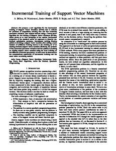
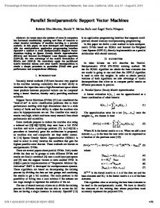
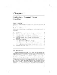
Figure 4: (a) A sub-optimal solution where the non- lled points have � = 0 but are violating optimality conditions by being inside the �1 area. (b) The decision surface gets rede ned. Since no points with � = 0 are inside the �1 area, the solution is optimal. Notice that the size of the margin has decreased, and the shape of the decision surface has changed. The computational results that we present in this section have been obtained using real data from our Face Detection System, which is described in Section 4. Figure 5 shows the training time and the number of support vectors obtained when training the system with 5,000, 10,000, 20,000, 30,000, 40,000, 49,000, and 50,000 data points. We must emphasize that the last 1,000 data points were collected in the last phase of bootstrapping of the Face Detection System, and therefore make the training process harder, since they correspond to errors obtained with a system that was already very accurate. Figure 6 shows the relationship between the training time and the number of support vectors, as well as the number of global iterations (the number of times the decomposition algorithm calls the solver). Notice the smooth relation between the number of support vectors and the training time, and the jump from 11 to 15 global iterations as we go from 49,000 to 50,000 samples. This increase is responsible for the increase in the training time. The system, using a working set of 1200 variables was able to solve the 50,000 data points problem using only 25Mb of RAM. Figure 7 shows the e�ect on the training time due to the parameter Newlimit and the size of the working set, using 20,000 data points. Notice the clear improvement as Newlimit is increased. This improvement suggests that in some way, the faster new violating data points are brought into the working set, the faster the decision surface is de ned, and optimality is reached. Notice also that, if the working set is too small or too big compared to the number of support vectors (746 in the case of 20,000 samples), the training time increases. In the rst case, this happens because the algorithm can only incorporate new points slowly, and in the second case, this happens because the solver takes longer to solve the subproblem as the size of the working set increases.
3.3 Improving the Training of SVM: Future Directions
The algorithm described in Section 3.2.3 suggests two main areas where improvements can be made through future research. These two areas are: 25
5
1000
4.5 900 4 Number of Support Vectors
Time (hours)
3.5 3 2.5 2 1.5
800
700
600
500
1 400 0.5 0 0
0.5
1
1.5
2
2.5 3 3.5 Number of Samples
(a)
4
4.5
300 0
5 4
x 10
0.5
1
1.5
2
2.5 3 3.5 Number of Samples
(b)
4
4.5
5 4
x 10
Figure 5: (a) Training Time on a SPARCstation-20. (b) Number of Support Vectors obtained after Training 1. The Solver: The second-order variant of the reduced gradient method implemented by MINOS 5.4 has given very good results so far in terms of accuracy, robustness and performance. However, this method is a general nonlinear optimization method that is not designed in particular for quadratic programs, and in the case of SVM's, is not designed in particular for the special characteristics of the problem. Having as a reference the experience obtained with MINOS 5.4, new approaches to a tailored solver through, for example, projected Newton �2] or interior point methods �7], should be attempted. At this point it is not clear whether the same type of algorithm is appropriate for all stages of the solution process. To be more speci c, it could happen that an algorithm performs well with few non-zero variables at early stages, and then is outperformed by others when the number of non-zero variables reaches some threshold. In particular, we learned that the number of non-zero variables that satisfy 0 < �i < C has an important e�ect on the performance of the solver. 2. The Pivoting Strategy: This area o�ers great potential for improvements through some ideas we plan to implement. The improvements are based on some qualitative characteristics of the training process that have been observed:
During the execution of the algorithm, as much as 40% of the computational e�ort is dedicated to the evaluation of the optimality conditions. At nal stages, it is common to have all the data points evaluated, yet only to collect very few of them to incorporate them to the working set.
Only a small portion of the input data is ever brought into the working set (about 16% in the case of the face detection application).
Out of the samples that ever go into the working set, about 30% of them enter and exit this set at least once. These vectors are responsible for the rst characteristic mentioned above. Possible future strategies that exploit these characteristics are:
Keep a list or le with all or part of the input vectors that have exited the working set. At the pricing stage, when the algorithm computes the optimality conditions, evaluate these data 26
16
5 4.5
14
4 Number of Global Iterations
12
Time (hours)
3.5 3 2.5 2 1.5
10
8
6
4
1 2
0.5 0 300
400
500
600 700 800 Number of Support Vectors
900
0 0
1000
(a)
0.5
1
1.5
2
2.5 3 3.5 Number of Samples
(b)
4
4.5
5 4
x 10
Figure 6: (a) Number of Support Vectors versus Training Time on a SPARCstation-20. Notice how the Number of support vectors is a better indicator of the increase in training time than the number of samples alone. (b) Number of global iterations performed by the algorithm. Notice the increase experimented when going from 49000 to 50000 samples. This increase in the number of iterations is responsible for the increase in the training time poits before other data points to determine the entering vectors. This strategy is analogous to one sometimes used in the revised simplex method where the algorithm keeps track of the basic variables that have become non-basic. In the case of training of SVM's, the geometric interpretation of this heuristic is to think that if a point was a support vector at some iteration, it was more or less close to the boundary between the classes, and as this boundary is re ned or �ne-tuned, it is possible for it to switch from active to non-active several times. This heuristic could be combined with main memory and cache management policies used in computer systems.
During the pricing stage, instead of bringing into the working set the rst k points that violate optimality conditions, we could try to determine r violating data points, with r > k and choose from these the k most violating points. This is done under the geometric idea that the most violating points help in de ning the decision surface faster and therefore save time in future iterations.
These last two approaches can be combined by keeping track not only of the points exiting the working set, but also of the remaining violating data points as well. So far in the description and implementation of the decomposition algorithm, we have assumed that enough memory is available to solve a working set problem that contains all of the support vectors. However, some applications may require more support vectors than the available memory can manage. One possible approach that can be taken is to approximate the optimal solution by the best solution that can be obtained with the current working set size. The present algorithm and implementation can be easily extended to handle this situation by replacing support vectors with 0 < �i < C with new data points. Other more complex approaches that can be pursued to obtain an optimal solution should be the subject of future research. 27
14
2 1.9
12 1.8 1.7 Time (hours)
Time (hours)
10
8
6
1.6 1.5 1.4 1.3
4
1.2 2 1.1 0 0
100
200
300
400
500 600 Newlimit
700
800
900
1 800
1000
(a)
1000
1200
1400 Working Set size
1600
1800
2000
(b)
Figure 7: (a) Training time for 20,000 samples with di�erent values of Newlimit, using a working set of size 1000 and Lookahead=10,000. (b) Training time for 20,000 samples with di�erent sizes of the working set, using Newlimit=size of the working set, and Lookahead=10,000.
4 SVM Application: Face Detection in Images
This section introduces a Support Vector Machine application for detecting vertically oriented and unoccluded frontal views of human faces in grey level images. It handles faces over a wide range of scales and works under di�erent lighting conditions, even with moderately strong shadows. The face detection problem can be de ned as follows: Given as input an arbitrary image, which could be a digitized video signal or a scanned photograph, determine whether or not there are any human faces in the image, and if there are, return an encoding of their location. The encoding in this system is to t each face in a bounding box de ned by the image coordinates of the corners. Face detection as a computer vision task has many applications. It has direct relevance to the face recognition problem, because the rst important step of a fully automatic human face recognizer is usually identifying and locating faces in an unknown image. Face detection also has potential application in human-computer interfaces, surveillance systems, census systems, etc. From the standpoint of this paper, face detection is interesting because it is an example of a natural and challenging problem for demonstrating and testing the potentials of Support Vector Machines. There are many other object classes and phenomena in the real world that share similar characteristics, for example, tumor anomalies in MRI scans, structural defects in manufactured parts, etc. A successful and general methodology for nding faces using SVM's should generalize well for other spatially well-de ned pattern and feature detection problems. It is important to remark that face detection, like most object detection problems, is a di�cult task due to the signi cant pattern variations that are hard to parameterize analytically. Some common sources of pattern variations are facial appearance, expression, presence or absence of common structural features, like glasses or a moustache, light source distribution, shadows, etc. This system works by testing candidate image locations for local patterns that appear like faces using a classi cation procedure that determines whether or not a given local image pattern is a face or not. 28
Therefore, the face detection problem is approached as a classi cation problem given by examples of 2 classes: faces and non-faces.
4.1 Previous Systems
The problem of face detection has been approached with di�erent techniques in the last few years. This techniques include Neural Networks �4] �19], detection of face features and use of geometrical constraints �27], density estimation of the training data �14], labeled graphs �12] and clustering and distribution-based modeling �22]�21]. Out of all these previous works, the results of Sung and Poggio �22]�21], and Rowley et al. �19] re"ect systems with very high detection rates and low false positive detection rates. Sung and Poggio use clustering and distance metrics to model the distribution of the face and non-face manifold, and a Neural Network to classify a new pattern given the measurements. The key of the quality of their result is the clustering and use of combined Mahalanobis and Euclidean metrics to measure the distance from a new pattern and the clusters. Other important features of their approach is the use of non-face clusters, and the use of a bootstrapping technique to collect important non-face patterns. One drawback of this technique is that it does not provide a principled way to choose some important free parameters like the number of clusters it uses. Similarly, Rowley et al. have used problem information in the design of a retinally connected Neural Network that is trained to classify faces and non-faces patterns. Their approach relies on training several NN emphasizing subsets of the training data, in order to obtain di�erent sets of weights. Then, di�erent schemes of arbitration between them are used in order to reach a nal answer. The approach to the face detection system with a SVM uses no prior information in order to obtain the decision surface, this being an interesting property that can be exploited in using the same approach for detecting other objects in digital images.
4.2 The SVM Face Detection System
This system, as it was described before, detects faces by exhaustively scanning an image for face-like patterns at many possible scales, by dividing the original image into overlapping sub-images and classifying them using a SVM to determine the appropriate class, that is, face or non-face. Multiple scales are handled by examining windows taken from scaled versions of the original image. Clearly, the major use of SVM's is in the classi cation step, and it constitutes the most critical and important part of this work. Figure 9 gives a geometrical interpretation of the way SVM's work in the context of face detection. More speci cally, this system works as follows: 1. A database of face and non-face 19 19 pixel patterns, assigned to classes +1 and -1 respectively, is trained on, using the support vector algorithm. A 2nd-degree polynomial kernel function and an upper bound C = 200 are used in this process obtaining a perfect training error. 2. In order to compensate for certain sources of image variation, some preprocessing of the data is performed:
Masking: A binary pixel mask is used to remove some pixels close to the boundary of the window pattern allowing a reduction in the dimensionality of the input space from 19 19=361 to 283. This step is important in the reduction of background patterns that introduce unnecessary noise in the training process.
Illumination gradient correction: A best- t brightness plane is subtracted from the unmasked window pixel values, allowing reduction of light and heavy shadows.
Histogram equalization: A-histogram equalization is performed over the patterns in order to compensate for di�erences in illumination brightness, di�erent cameras response curves, etc. 29
3. Once a decision surface has been obtained through training, the run-time system is used over images that do not contain faces, and misclassi cations are stored so they can be used as negative examples in subsequent training phases. Images of landscapes, trees, buildings, rocks, etc., are good sources of false positives due to the many di�erent textured patterns they contain. This bootstrapping step, which was successfully used by Sung and Poggio �22] is very important in the context of a face detector that learns from examples because:
Although negative examples are abundant, negative examples that are useful from a learning point of view are very di�cult to characterize and de ne.
By approaching the problem of object detection, and in this case of face detection, by using the paradigm of binary pattern classi cation, the two classes, object and non-object are not equally complex since the non-object class is broader and richer, and therefore needs more examples in order to get an accurate de nition that separates it from the object class. Figure 8 shows an image used for bootstrapping with some misclassi cations, that were later used as negative examples. 4. After training the SVM, we incorporate it as the classi er in a run-time system very similar to the one used by Sung and Poggio �22]�21] that performs the following operations:
Re-scale the input image several times.
Cut 19 19 window patterns out of the scaled image.
Preprocess the window using masking, light correction and histogran equalization.
Classify the pattern using the SVM.
If the class corresponds to a face, draw a regtangle aroung the face in the output image.
4.2.1 Experimental Results
To test the run-time system, we used two sets of images. The set A, contained 313 high-quality images with same number of faces. The set B, contained 23 images of mixed quality, with a total of 155 faces. Both sets were tested using our system and the one by Sung and Poggio �22]�21]. In order to give true meaning to the number of false positives obtained, it is important to state that set A involved 4,669,960 pattern windows, while set B 5,383,682. Table 5 shows a comparison between the 2 systems. Test Set A Test Set B Detection Rate False Detections Detection Rate False Detections Ideal System 100 % 0 100% 0 SVM 97.12 % 4 74.19% 20 Sung and Poggio 94.57 % 2 74.19% 11 Table 5: Performance of the SVM face detection system Figures 10, 11, 12, 13, 14 and 15 present some output images of our system. These images were not used during the training phase of the system.
4.3 Future Directions in Face Detection and SVM Applications
Future research in SVM application can be divided into three main categories or topics: 1. Simpli�cation of the SVM: One drawback for using SVM in some real-life applications is the large number of arithmetic operations that are necessary to classify a new input vector. Usually, this number is proportional to the dimension of the input vector and the number of support vectors obtained. In the case of face detection, for example, this is � 283,000 multiplications per pattern! The reason behind this overhead is in the roots of the technique, since SVM's de ne the decision surface by explicitly using data points. This situation causes a lot of redundancy in most cases, and 30
can be solved by relaxing the constraint of using data points to de ne the decision surface. This is a topic of current research conducted by Burges �6] at Bell Laboratories, and it is of great interest for us, because in order to simplify the set of support vectors, one needs to solve highly-nonlinear constrained optimization problems. Since a closed form solution exists for the case of kernel functions that are 2nd. degree polynomials, we are using a simpli ed SVM �6] in our current experimental face detection system that gains an acceleration factor of 20, without degrading the quality of the classi cations. 2. Detection of other objects: We are interested in using SVM's to detect other objects in digital images, like cars, airplanes, pedestrians, etc. Notice that most of these objects have very di�erent appearance, depending on the viewpoint. In the context of face detection, an interesting extension that could lead to better understanding and approach to other problems, is the detection of tilted and rotated faces. It is not clear at this point, whether these di�erent view of the same object can be treated with a single classi er, or if they should be treated separately. 3. Use of multiple classi�ers: The use of multiple classi ers o�ers possibilities that can be faster and/or more accurate. Rowley et al. �19] have successfully combined the output from di�erent neural networks by means of di�erent schemes of arbitration in the face detection problem. Sung and Poggio �22]�21] use a rst classi er that is very fast as a way to quickly discard patterns that are clearly non-faces. These two references are just examples of the combination of di�erent classi ers to produce better systems. Our current experimental face detection system performs an initial quick-discarding step using a SVM trained to separate clearly non-faces from probable faces using just 14 averages taken from di�erent areas of the window pattern. This classi cation can be done about 300 times faster and is currently discarding more than 99% of input patterns. More work will be done in the near future in this area. The classi ers to be combined do not have to be of the same kind. An interesting type of classi er that we will consider is Discriminant Adaptative Nearest Neighbor due to Hastie et al. �11]�10].
5 Conclusions In this paper we presented a novel decomposition algorithm to train Support Vector Machines. We have successfully implemented this algorithm and solved large dataset problems using acceptable amounts of computer time and memory. Work in this area can be continued, and we are currently studying new techniques to improve the performance and quality of the training process. The Support Vector Machine is a very new technique, and, as far as we know, this paper presents the second problem-solving application to use SVM, after Vapnik et al. �5, 8, 24] used it in the character recognition problem, in 1995. Our Face Detection System performs as well as other state-of-the-art systems, and has opened many interesting questions and possible future extensions. From the object detection point of view, our ultimate goal is to develop a general methodology that extends the results obtained with faces to handle other objects. From a broader point of view, we also consider interesting the use of the function approximation or regression extension that Vapnik �24] has done with SVM, in many di�erent areas where Neural Networks are currently used. Finally, another important contribution of this paper is the application of OR-based techniques to domains like Statistical Learning and Arti cial Intelligence. We believe that in the future, other tools like duality theory, interior point methods and other optimization techniques and concepts, will be useful in obtaining better algorithms and implementations with a solid mathematical background. 31
References
�1] M. Bazaraa, H. Sherali, and C. Shetty. NonLinear Programming Theory and Algorithms. J. Wiley, New York, 2nd edition, 1993. �2] D. Bertsekas. Projected newton methods for optimization problems with simple constraints. SIAM J. Control and Optimization, 20(2):221{246, March 1982. �3] B.E. Boser, I.M. Guyon, and V.N. Vapnik. A training algorithm for optimal margin classi er. In Proc. 5th ACM Workshop on Computational Learning Theory, pages 144{152, Pittsburgh, PA, July 1992. �4] G. Burel and D. Carel. Detection and localization of faces on digital images. Pattern Recognition Letters, 15:963{967, 1994. �5] C. Burges and V. Vapnik. A new method for constructing arti cial neural networks. Technical report, AT&T Bell Laboratories, 101 Crawfords Corner Road Holmdel NJ 07733, May 1995. �6] C.J.C. Burges. Simpli ed support vector decision rules, 1996. �7] T. Carpenter and D. Shanno. An interior point method for quadratic programs based on conjugate projected gradients. Computational Optimization and Applications, 2(1):5{28, June 1993. �8] C. Cortes and V. Vapnik. Support vector networks. Machine Learning, 20:1{25, 1995. �9] F. Girosi. An equivalence between sparse approximation and Support Vector Machines. A.I. Memo 1606, MIT Arti cial Intelligence Laboratory, 1997. (available at the URL: http://www.ai.mit.edu/people/girosi/svm.html). �10] T. Hastie, A. Buja, and R. Tibshirani. Penalized discriminant analysis. Technical report, Statistics and Data Analysis Research Department, AT&T Bell Laboratories, Murray Hill, New Jersey, May 1994. �11] T. Hastie and R. Tibshirani. Discriminat adaptative nearest neighbor classi cation. Technical report, Department of Statistics and Division of Biostatistics, Stanford University, December 1994. �12] N. Kr(uger, M. P(otzsch, and C. v.d. Malsburg. Determination of face position and pose with learned representation based on labled graphs. Technical Report 96-03, Ruhr-Universit(at, January 1996. �13] J. Mercer. Functions of positive and negative type and their connection with the theory of integral equations. Philos. Trans. Roy. Soc. London, A 209:415{446, 1909. �14] B. Moghaddam and A. Pentland. Probabilistic visual learning for object detection. Technical Report 326, MIT Media Laboratory, June 1995. �15] E.H. Moore. On properly positive Hermitian matrices. Bull. Amer. Math. Soc., 23(59):66{67, 1916. �16] J. Mor#e and G. Toraldo. On the solution of large quadratic programming problems with bound constraints. SIAM J. Optimization, 1(1):93{113, February 1991. �17] B. Murtagh and M. Saunders. Large-scale linearly constrained optimization. Mathematical Programming, 14:41{72, 1978. �18] B. Murtagh and M. Saunders. MINOS 5.4 User's Guide. System Optimization Laboratory,Stanford University, Feb 1995. �19] H. Rowley, S. Baluja, and T. Kanade. Human face detection in visual scenes. Technical Report CMU-CS-95-158R, School of Computer Science, Carnegie Mellon University, November 1995. 32
�20] J. Stewart. Positive de nite functions and generalizations, an historical survey. Rocky Mountain J. Math., 6:409{434, 1976. �21] K. Sung. Learning and Example Selection for Object and Pattern Detection. PhD thesis, Massachusetts Institute of Technology, Arti cial Intelligence Laboratory and Center for Bilogical and Computational Learning, December 1995. �22] K. Sung and T. Poggio. Example-based learning for view-based human face detection. A.I. MEMO 1521, C.B.C.L Paper 112, December 1994. �23] V. Vapnik. Estimation of Dependences Based on Empirical Data. Springer-Verlag, 1982. �24] V. Vapnik. The Nature of Statistical Learning Theory. Springer-Verlag, 1995. �25] V. N. Vapnik and A. Y. Chervonenkis. On the uniform convergence of relative frequences of events to their probabilities. Th. Prob. and its Applications, 17(2):264{280, 1971. �26] V.N. Vapnik and A. Ya. Chervonenkis. The necessary and su�cient conditions for consistency in the empirical risk minimization method. Pattern Recognition and Image Analysis, 1(3):283{305, 1991. �27] G. Yang and T. Huang. Human face detection in a complex background. Pattern Recognition, 27:53{63, 1994. �28] W.Y. Young. A note on a class of symmetric functions and on a theorem required in the theory of integral equations. Philos. Trans. Roy. Soc. London, A 209:415{446, 1909. �29] G. Zoutendijk. Methods of Feasible Directions. D. Van Norstrand, Princeton, N.J., 1960.
33
Figure 8: Some false detections obtained with the rst version of the system. This false positives were later used as negative examples ( class -1 ) in the training process
34
NON-FACES
FACES Figure 9: Geometrical Interpretation of how the SVM separates the face and non-face classes. The patterns are real support vectors obtained after training the system. Notice the small number of total support vectors and the fact that a higher proportion of them correspond to non-faces.
35
Figure 10: Faces 36
Figure 11: Faces
37
Figure 12: Faces
38
Figure 13: Faces
39
Figure 14: Faces 40
Figure 15: Faces 41