To uniformly express temporal and provenance queries we introduce evo-path .... before the change and the object version after the change. Evolution .... &4. &5. &1. &50. &51. Web DataBank A. Web DataBank B. T=start ... ... "m1". 9. 100. &6. ID ... collision with miRNA âm2â, which on T=1 starts at position 110. Therefore, the ...
Supporting Complex Changes in Evolving Interrelated Web Databanks Yannis Stavrakas, George Papastefanatos Institute for the Management of Information Systems Athens, Greece {yannis,gpapas}@imis.athena-innovation.gr
Abstract. In this paper we deal with problems occurring in evolving interrelated Web databanks. Examples of such databanks are networks of interlinked scientific repositories on the Web, managed independently by cooperating research groups. We argue that changes should not be treated solely as transforming operations, but rather as first class citizens retaining structural, semantic and temporal characteristics. We propose a graph model called evograph for capturing in a coherent way the inherent relationship between evolving data and changes applied on them. Evo-graph represents changes as arbitrarily complex objects, similarly to data objects. We discuss the temporal characteristics of the evo-graph, and show how the evo-graph can provide past snapshots of the data. To uniformly express temporal and provenance queries we introduce evo-path, a path expression language based on XPath. Evo-path takes advantage of complex changes in the evo-graph in order to answer queries that interpret and elucidate data evolution. Keywords: Evolution of semistructured data, change-centric management
1
Introduction
The wide availability and fast publishing of information enabled by the Web unlocked new potential as well as new problems for data management. Particularly, an emerging issue concerns collections of Web data (often scientific) that evolve independently, but remain in some ways interconnected. Those interconnections stem from the cooperative nature of the teams maintaining the collections. Consider, for example, biology research communities [2,13], that produce, consume, and archive rapidly large amounts of data. Scientific communities like that rely increasingly on the Web for collaboration, through the publication and integration of experimental and research results. Moreover, scientists in those communities would often like to review how and why the recorded data have evolved, in order to compare and reevaluate previous and current conclusions. Such an activity may require a search that moves backwards and forwards in time, spreads across various databanks, and performs complex queries on the semantics of the changes that modified the data. In
those cases, simply revising past document snapshots and differences between versions may not be enough. As a simplified example, consider two Web databanks, A and B, maintained by two biology research teams. Databank A is an authoritative source in miRNAs. A miRNA is a part of the DNA chain associated with the production of proteins, and is defined by a start point in the chain and a length. Under certain circumstances different miRNAs can attach themselves at different points on the DNA chain, causing important effects. Databank B contains results of experiments and performs time-consuming calculations for estimating these possible points of attachment for every miRNA. These points of attachment are called targets. In Fig. 2, databank A models a miRNA as an ID, a position, and a length, while databank B contains “predictions” that associate miRNA IDs with possible targets. Databank B, like many other databanks, relies on databank A to get the most recent developments. Knowledge on miRNAs advances rapidly, and A changes often to reflect this. A miRNA in A may change name and properties, split into two distinct miRNAs, merge with another to form a new miRNA, etc. Other databanks, like B, have to check the contents of A regularly, and synchronize their contents with those of A. Research teams will probably need to repeat experiments or calculations in order to adapt to the new facts exposed in A. Such databanks form a network of interdependent data that evolve independently. In this network, issues of evolution and provenance are closely related; evolution information is needed in order to be able to answer provenance queries, not only within a single databank, but across many databanks as well. Interdependencies among databanks occur because it is common practice for scientific databanks to copy information objects from other scientific databanks. Until now significant work has been done separately on evolution [5,8,14] and provenance [4] of XML and semistructured data. Specifically in [4] the issue of interdependent Web data has been recognized and studied. However, previous approaches do not cover all the aspects of the problem presented above, since each of them focuses on the specific questions regarding the framework it addresses. From the example above it becomes clear that in some cases evolution cannot be studied separately from provenance. In this paper we argue that in cooperative systems where evolution and provenance issues are paramount, changes should not be treated solely as transformation operations on the data, but rather as first class citizens retaining structural, semantic, and temporal characteristics. Modeling complex changes explicitly can leverage a number of new interesting queries, and provide additional semantic information for interpreting past data. We propose a graph model called evo-graph for capturing in a coherent way the inherent relationship between evolving data and changes applied on them. We employ this model for representing simple as well as composite evolution operations. We discuss in detail the temporal characteristics of the evo-graph, and show how the evo-graph can provide past snapshots of the data. Finally, we introduce evo-path, a path expression language for evo-graph that extends XPath. Evo-path takes advantage of the complex changes in the evo-graph in order to answer queries about the provenance of data, and the interpretation of data evolution.
The structure of the paper is as follows. In section 2 we discuss related work. In section 3 we define evo-graph and give an extended example based on databanks A and B mentioned earlier. In section 4 we present the temporal properties of the evograph, and show how temporal snapshots can be extracted from the evo-graph. In section 5 we introduce evo-path and give example queries that take advantage of the complex changes represented in evo-graph. Finally, section 6 concludes the paper.
2
Related Work
Modeling and managing evolving Web data have recently attracted a growing interest in the database research community. We classify the various approaches as follows. Change Detection, Versioning and XML Diffs. In one of the early approaches [5], the authors deal with the representation of changes in semistructured data, and propose DOEM, an extension of OEM capable of representing changes as annotations on nodes and edges. They propose a query language, named CHOREL, for retrieving information related to the history of nodes and edges, exploiting the change annotations. In [14] a change-centric method for managing versions in XML data is presented. The authors employ a diff algorithm for detecting changes between two versions of a document. Changes are represented either as edit scripts, simple deltas or completed deltas. A similar approach is introduced in [7,8], where instead of deltas calculations, a referenced-based identification of each object is used across different versions. New versions hold only the elements that are different from the previous version whereas a reference is used for pointing to the unchanged elements of past versions. In [11] the authors propose MXML, a extension of XML that uses context information to express time and models multifaceted documents. Other approaches, such as the X-Diff algorithm [19] and [6], focus mainly on the detection and less on the representation of the changes between two documents. Recently, there are works that deal with the detection of changes in semantic data, such as [16]. Temporal approaches to evolving data. An annotated bibliography on temporal and evolution aspects for Web data is presented in [12]. Most temporal approaches [1,5] enrich data elements with temporal attributes for holding valid and / or transaction time, and extend query syntax with conditions on the time validity of data [9]. In [17], a temporal model for XML is introduced, which models an XML document as a directed graph, and attaches transaction time information at the edges of the graph. The authors provide techniques for implementing the model with XML, for indexing temporal documents, and for performing temporal queries. Techniques for evaluating temporal queries on semistructured data are presented in [10,18]. In [10] the authors propose a temporal query language for adding valid time support in XQuery. In [18] the notion of a temporally grouped data model is employed for uniformly representing and querying successive versions of a document. In a more recent work [15], the authors extend this technique for publishing the history of a relational database in XML. The authors introduce the PRIMA system, where they employ a set of schema modification operators (SMOs) for representing the mappings between successive schema versions.
Archiving and Provenance in semistructured data. Work on data provenance has been mainly directed towards relational data. As far as XML and semistructured data are concerned, the archiving and management of curated databases is addressed in [3]. The authors develop an archiving technique for scientific data that uses timestamps for each version, whereas all versions are merged into one hierarchy. By identifying the semantic continuity of elements and merging them into one data structure, this approach is capable of providing meaningful change descriptions. The authors exploit the archive to answer certain temporal queries, such as retrieval of any specific version, and retrieval of the history of an element. In [4] the authors provide a technique for modeling and recording provenance information in curated databases. They consider evolution operations that span across multiple databases, such as copying and pasting data from one database to another. Compared to the above approaches, ours has the following distinctive characteristics. First of all, we do not detect changes through diffs, but rather we assume that changes are introduced in our model as they occur. Changes in our approach are complex objects operating on data, and exhibit structural, semantic, and temporal properties: they can be part of other changes, correlate to each other, be transactional, long-termed or instant. These properties allows our evolution model to answer queries about “what” has evolved over time, but also to provide information about “why” and “how” data have evolved. Second of all, temporal information is assigned to the changes rather than the data, and characterizes the time that a change occurred. Based on this, the validity timespan of each version of an evolving object is determined. As a result, temporal conditions can be expressed uniformly in both data and changes. Third of all, our approach employs the same principles for modeling evolution events within a single database, as well as capturing interdependencies between disparate databases. Structuring changes into complex objects enable us to address provenance and evolution issues in a uniform manner.
3
Modeling Evolution using Complex Changes
In this section we propose evo-graph, a graph model for interrelated evolving data, where changes are given equal importance as data. We present a set of basic change operations, we define evo-graph and discuss how it is constructed, and we give an example of using evo-graph in an extensive biological data scenario. 3.1
Evo-graph: Changes as First-class Citizens
A number of data models have been proposed in the past for semistructured data and XML [5,21]. In general, those models represent data using labeled rooted directed graphs, with values on the leaves. In this paper, we assume that Web data are represented at any given instance by a rooted acyclic graph, called from now on by the generic name snap-graph (see Fig. 2). A snap-graph consists of data nodes (complex and atomic), and edges connecting the nodes. In addition to the snap-graph components, we introduce the following new concepts in evo-graph (see Fig. 3):
Change nodes are nodes that represent change events: basic change operations, and complex changes. Change nodes appear as triangles, to distinguish from conventional circular data nodes. Change edges connect a complex change node to the (complex or atomic) change nodes it consists of. Change edges are represented by dashed lines. Evolution edges connect each change node with two data nodes: the object version before the change and the object version after the change. Evolution edges appear as thick lines. The evo-graph is constructed step by step, as changes occur at the current version of the snap-graph. We will use the following five basic change operations for the snap-graph: create: creates a new child node, and connects it with the parent node. add: adds an edge between two existing nodes, effectively adding a child node. remove: removes an edge, deleting a child. update: updates the value of an atomic node. clone: creates a deep copy B of a subtree A, and connects B under the same parent node as A. snap-model
snap-model
evo-model
T=start
T=1
T=1
A
A
&1
&1
&1
update (&2, 10) at T=1
update &4
B
B &2
&3
5
10
B
1
B &2
&3
5
10
snap-model
snap-model
evo-model
T=start
T=8
T=8
A
A
&1
A
&1
&1 update &6
remove (&4) at T=8 B
C
B
&2
C
D &3
&4
B
&2
C &3
8 &5
&2
D &3
&4
Fig. 1. Modeling of basic change operation with evo-graph
Our approach is to create a new version of an object in the evo-graph whenever a change occurs to a child of that object. Each change creates a new change node and a
new evolution edge, connecting the previous version with the new version of the object. Fig. 1 shows how the basic change operations update and remove are represented in the evo-graph. Nodes contain their respective node ID, and node labels are placed next to each node. In the case of remove, when node &4 is removed from the children of node &2, a new version of node &2 with ID &5 is created in the evograph to reflect this change. As a general rule, changes that affect child nodes create new versions of the parent nodes. The same holds for update, since the atomic node &2 can be considered as the parent of an implied “value node”. The definition of evo-graph follows. Evo-graph definition. The evo-graph is a finite directed acyclic graph G = (VD, VC, ED, EC, EE, rD, rC, fL, fV), such that: 1. Data nodes are divided into complex and atomic: VD = VDc VDa. 2. Change nodes are divided into complex and atomic: VC = VCc VCa. 3. Data edges depart from every complex data node, ED (VDc VD). Only one data edge may exist between two nodes. 4. Changes edges depart from every complex change node, EC (VCc VC), with each vC (VC - rC) having exactly one parent. 5. Evolution edges are directed edges that connect one change node with two data nodes: EE (VD VC VD). For every change node vC VC there exists in EE an evolution edge eE = (vD, vC, vD ), with fL(vD) = fL(vD ). The following directions are implied by eE: vD vD , vD vC, and vC vD . 6. rD VD is the data root, with the property that there exists a path formed by data edges and evolution edges from rD to every other node in VD . 7. rC VC is the change root, with the property that there exists a path formed by change edges from rC to every other node in VC. 8. fL is a function that assigns labels to nodes, such that: ─ fL(x) C if x VCa, where C is the set of names of the basic change operations, and ─ fL(x) L if x VCc VD, where L is the set of all other labels. 9. fV is a function that assigns values to nodes, such that: ─ fV(x) ─ fV(x)
A if x T if x
VDa, where A is the set of atomic values, and VCa, where T is the set of timestamps.
The number assigned to each atomic change represents the time instance the change occurred. We assume a linear time domain and two special time instances: start, representing the beginning of time, and now, representing the current moment. The next section presents how those time instances propagate to complex changes and to the rest of the evo-graph, in order to get temporal snapshots of the data. Intuitively, the evo-graph consists of two correlated graphs: a data graph, and a tree of changes. The data graph defines the structure of data, while the change graph defines the structure of changes on data. These two graphs interconnect by means of evolution edges, which denote the data object affected by each change. Consequently there are two roots, the data root and the change root. The change root is assumed to
be always linked to an evolution edge that originates from the version T=start of the data root, and points to the version T=now of the data root. Moreover, there are two types of paths: the change paths that follow successive change edges, and the data paths that follow successive data and / or evolution edges. T=start
Web DataBank A
Web DataBank B
...
...
miRNAs
predictions &50
&1
miRNA
miRNA
&2
pos
ID
length
prediction &6
pos
ID
&51
length
&3
&4
&5
&7
&8
&9
"m1"
100
9
"m2"
110
30
Fig. 2. State of Web databanks A and B at T=start
The main objective of the evo-graph is to represent arbitrarily complex changes. The semantics of a complex change is implied by the structure of the change, as defined by the users of the databank. An atomic change can only represent one of the basic change operations, however there is no restriction on how atomic changes are combined to form complex changes. Note that, as long as the set of basic change operations is complete (operations can lead the snap-graph to any possible state), the choice of basic change operations is not restricted by the evo-graph: alternative sets of may be adopted, while the properties of evo-graph remain largely insensitive to which set is selected. 3.2
Recording Evolution and Databank Interrelations Using Complex Changes
Based on the example introduced in section 1, in this section we present a simple scenario which demonstrates how the evo-graph can be used to record dependencies and changes in two evolving interrelated Web databanks that publish bioscientific data: databank A, and databank B. Through this example we attempt to establish the importance of treating complex changes as first class citizens, since they convey indispensable semantic information for interpreting the evolution of data as well as the reasons for their current and previous states.
We assume that databank A initially contains only two miRNAs, while databank B contains a single prediction object without any data yet, as it is depicted in Fig. 2. ... T=3
Web DataBank A m1-lengh-change &19 miRNAs &18
&1
miRNAs
pos-len-update &17 miRNA &2
miRNA
&6
&16 miRNA
update update
&11 length
1 &5
ID
length
&15
&10
length update
pos &3
&4
9
19
&13 pos
"m1"
100 ID
pos
2 &8
&12
110
120
3
length
&9
&14
30
20
&7 "m2"
Fig. 3. Evo-graph for Web databank A at T=3
Fig. 3 shows the evo-graph for databank A at T=3. For simplicity, the data root and the change root are omitted. At time instance 1 (T=1) the length of the miRNA with ID “m1” is updated from 9 to 19. This basic change operation is expressed by the change node &11 that creates a new version of the length (node &10). For simplicity, the arguments of change operations are implied and do not appear on the figures. After this update, “m1” occupies the positions 100 to 119. This, however, causes a collision with miRNA “m2”, which on T=1 starts at position 110. Therefore, the start position of “m2” (node &8) must be updated as a consequence of the change occurred to “m1”. For the sake of the example, we assume that the end position of “m2” at the DNA chain remains fixed. Therefore, an update of the start position of “m2” must be followed by an update of its length, so that its end position remains the same. This is modeled by the complex change pos-len-update that appears in Fig. 3 as node &17. This complex change creates a new version of the specific miRNA, and consists of two atomic changes: an update of the start position of “m2” (node &13 introduces node &12), and an update on the length of “m2” (node &15 introduces node &14).
Change nodes &11 and &17 are further composed into the complex operation m1length-change, represented by node &19. This operation is associated with node &1 and causes the creation of a new version of the miRNAs node (node &18). Complex change nodes can represent relationships between changes that take place in disparate places of the databank, and would otherwise be treated as unrelated. In this way, it is possible to model any change operation, like for instance, move, split, merge, etc. T=7
...
Web DataBank A
... predictions
miRNAs &1
Web DataBank B
...
&50
copy
create &54
miRNA
miRNA
&6
&2
&62
4 &51
... pos
ID &3
prediction
&53 prediction
&60 prediction
length &4
&5
target
ID
&52 "m1"
100
19
&57 "m1"
550
copy &62
add
clone &56 5
&53 prediction
remove &59
&61
6
7 &58
&55 prediction
prediction
&60 prediction
ID
target &52 550
&57 "m1"
Fig. 4. Evo-graph for Web databank B at T=7
Fig. 4 depicts the evo-graph for databank B at T=7. Databank B decides to include miRNA “m1”, and publish a prediction for its target. At T=4 a new target node is added under the prediction node in databank B. The new data node (&52) with label
target and value 550 is created by the basic change operation create, which is represented by the change node &54. Instead of placing node &52 under the existing prediction node &51, a new version of the prediction node is introduced (&53). Therefore, the change operation represented by &54 transforms the data node &51 to the data node &53 by creating the child node &52. Now that the target data is inserted, the next step is to insert the ID of the miRNA associated with this target. We assume that the ID in question is copied from databank A to databank B. It is common practice to copy data among Web databanks, which leads to a number of issues related to data provenance [4]. The main objective is to copy data from independently managed databanks, while maintaining evidence of this transaction. The copy change operation is a complex operation represented in Fig. 4 by the change node &62. The change node &62 transforms node &53 to node &60, by adding the child node &57, which is a copy of the node &3 in databank A. Due to space limitations, the copy operation is fully presented at the bottom of Fig. 4. It consists of three basic change operations, add, clone, and remove, that take place at T=5, T=6, and T=7 respectively. The basic change operation add connects a new version (&55) of the prediction node to the child node &3 of the databank A (we assume here a mechanism for referring to nodes residing at disparate sites). The basic change operation clone creates a (deep) copy of node &3 as node &57. Finally, the basic change operation remove deletes the edge from node &58 to node &3, leading to the final version of the prediction node (&60). Summarizing, this example demonstrates how the evo-graph models evolution using arbitrarily complex changes, with sub-changes applied to objects that can reside far from each other in the data graph. It also shows how the same principles can be used to create and maintain links between disparate databanks, as in the case of copying and pasting information.
4
Temporal Properties of the Evo-graph
Evo-graph captures in a uniform way multiple data versions along with the evolution operations applied on each version, and represents them in a coherent graph enriched with temporal information. A key difference from existing versioning and temporal approaches on XML and semistructured data is that the time dimension is not assigned on the data elements of the graph (i.e., data nodes and edges); instead it is the change nodes that retain and propagate all temporal information on the evo-graph. A timestamp t is assigned to each atomic change node VCa, denoting the time on which this change occurred. Two or more change nodes may have identical timestamps as long as they correspond to changes that occurred at the same time. In this section, we present the main mechanisms for propagating time information from the atomic change nodes towards the rest of the graph elements. Furthermore, we provide a technique for reducing the evo-graph to the snap-graph that holds under a given timestamp.
4.1
Propagation of Timespans
As already mentioned, each atomic change node in the evo-graph is assigned a timestamp denoting the time instance that the change occurred. The timestamp of a complex change is then considered to be the timestamp of its most “recent” child, and denotes the time instance the complex change is completed. Thus, timestamps propagate upwards in the change tree, imposing a partial order on changes. Notice that different change nodes with the same timestamp are allowed in our model, implying the concurrent occurrence of the respective changes. In this case, concurrent change nodes must not belong to the same direct parent, i.e., they cannot be siblings. Change timestamps determine the validity timespan of data nodes and data edges. Every change affects the validity timespan of the two data nodes it is connected with (through the respective evolution edge), in the sense that the previous version of an object stops being valid the moment a new version is created. Timespans propagate to child data nodes, since a child can only exist if it has a valid parent. In what follows we specify the process for obtaining the validity timespans for the data nodes in the evo-graph. We give two different procedures: one top-to-bottom, for batch processing the timespans of an evo-graph, and one incremental, for updating the timespans in the evo-graph after a single modification has taken place. We define timespans as unions of time intervals of the form [t1..t2) [t3..t4] …, and we use two special values, start and now, to represent the beginning of time and the current time, respectively. Note that intervals may be open or closed on the borders, excluding or including their left / right values. Top-to-bottom propagation. The top-to-bottom propagation goes through the entire graph and calculates all the timespans from scratch. It performs a DFS (depth first search) traversal on the graph starting from data root rD and assuming an initial timespan [start..now], and assigns a timespan to all nodes and edges. Whenever encountering a change node, the algorithm propagates the timestamp of the change node to the data nodes and edges of the graph. The steps of the algorithm are given below. ─ Step 1. Set as the current node the data root rD ─ Step 2. For each outgoing data edge ei=(rD,xi) ED set T(ei)=T(rD), i.e. the timespan of each node is propagated to all outgoing edges. ─ Step 3. Set T(xi)= T(xk,xi), i.e. the timespan of a node is equal to the union of the timespans of all incoming edges, or equivalently as stated in step 2 to the union of all timespans of its parents. ─ Step 4. If an evolution edge eev=(xi,c,x’i) EE exists, then for each outgoing evolution edge eev=(xi,c,x’i) EE with timestamp tc do steps 4a to 4d. ─ Step 4a.The timespan of xi becomes equal to T(xi)=T(xi) [0..tc). ─ Step 4b.The timespan of x’i becomes equal to T(x’i)=T(x’i) [tc..now]. ─ Step 4c. Consider xi as root and return to step 2, i.e. propagate the new timespan of xi towards the paths starting from this node. ─ Step 4d. Set xi = x’i and repeat step 4, i.e., check if an evolution edge starts from x’i. ─ Step 5. Else, consider xi as root and return to step 2.
The evo-graph of Fig. 3 is shown with time annotations in Fig. 5. ... Propagation of timestamps
m1-lengh-change &19 3 miRNAs
&18
&1
[s..3)
miRNAs [3..n] pos-len-update &17 3
miRNA [s..n]
miRNA [s..3)
&2
&6
&16 miRNA [3..n]
update update
&11 length [s..1) ID [s..n]
pos [s..n]
1 &5
&10
length [1..n]
&15 update
&3
&4
"m1"
100
9
19 pos [s..2) ID [s..n]
length [s..3)
&13 &8
pos &12 [2..n]
110
120
2
length [3..n]
3 &9
&14
30
20
&7 "m2"
Fig. 5. Time annotated evo-graph of Fig. 3
Incremental propagation. When a new change occurs on a node of the graph, the timestamp assigned to the new change node affects only the time validity of the previous and current version of the node sustaining the change. The incremental propagation adjusts the timespans of these nodes and propagates the new timespans to their descendants only. Let us assume that an evolution change c with timestamp tc is applied on node xi with a timespan T(xi), creating a new evolved node x’i and an evolution edge (xi,c,x’i). Then: ─ The timespan of xi becomes T(xi)=T(xi) [0..tc). The timespan is propagated to all accessible paths, considering xi as root and executing the topto-bottom propagation at step 2. ─ The timespan of x’i becomes T(x’i)=T(x’i) [tc..now]. Similarly, we consider x’i as root and propagate the timespan to all accessible paths. The assignment of timespan to graph elements can be optimized by omitting the step 4d that propagates downwards the two subtrees, and by retaining the timespans only for the nodes involved in an evolution edge. For all other nodes, we assume that they inherit the union of the timespans of their parents.
4.2
Snapshot Reduction of the Evo-graph
The temporal information on the evo-graph allow us to perform a special operation called snapshot reduction, for extracting the specific version holding under a given time instance. Snapshot reduction takes as input an evo-graph plus a time instance, and produces a snap-graph consisting only of those data nodes and data edges for which their validity timespan contains the given time instance. The algorithm is presented in Table 1. Table 1. Snapshot Reduction algorithm Input: an evo-graph G= (VD, VC, ED, EC, EE, rD, rC) a requested time instance t Output: a snapshot graph G’=(VD’,ED’) begin VD’ = rD get_snapshot(G, G’, t , rD) end get_snapshot(G, G’, t , x0) begin for each edge(x0,xi) ED { if eev=(xi,c,x’i) EE exists { xi=get_version(G,G’,t,xi)} if t T(xi){ ED’ = ED’ (x0,xi) if (xi VD’){ VD’=VD’ xi get_snapshot(G, G’, t , xi)}} } End
get_version(G, G’, t , xi) begin stack s, list visited s->put(xi) while(!s->empty){ s->pop(xi), visited->add(xi) if t T(xi): return(xi) else: for each (xi,c,x’i) EE { if x’i visited: s->put(x’i)} } end
The algorithm starts from the data root and calls the get_snapshot method, which performs a recursive DFS on the evo-graph. When a data node attached to an evolution edge is met, an inner DFS traversal (named get_version) is performed across the successive versions of this node for retrieving the version which is valid for the requested time instance. The algorithm connects this version with its parent, and continues the traversal downwards all paths starting from this node. The resulting snap-graph does not contain any change nodes or evolution edges, and can be easily transformed to XML format, following a non replicated top-down traversal [17]. The snap-graph for the time instance T=3 of the evo-graph in Fig. 5 is shown in Fig. 6.
... Snapshot for T=3 Web DataBank A &18
miRNA
ID
miRNA &2
&16
length
pos
miRNAs
ID
pos
length
&3
&4
&10
&7
&12
&14
"m1"
100
19
"m2"
120
20
Fig. 6. Snap-graph for T=3 of the evo-graph in Fig. 5
5
Introducing Evo-path Expressions
XPath (XML Path Language) [20] is a language proposed by W3C for addressing portions of a XML document. The basic structural unit of XPath is the XPath expression, which may return either a node-set, a string, a Boolean, or a number. The most common kind of XPath expression, which is used in XPath to select nodes or node-sets in an XML document, is the path expression (or location path expression). In this section we propose evo-path as an extension of XPath used to navigate through evo-graphs. Similarly to XPath, evo-path uses path expressions as a sequence of steps to get from one data node to another data node (or set of data nodes). In addition to XPath, evo-path uses constructs that allows the navigation through change nodes, plus predicates that express conditions on the connections between change nodes and data nodes (conditions on evolution edges). 5.1
Extending XPath for Accommodating Change Path Expressions
There are two kinds of path expressions in evo-paths: data path expressions, and change path expressions. Data path expressions start from the data root of the evo-graph and return data nodes. Similarly to XPath they are written as a sequence of location steps that get from one node (the current context node) to another node or set of nodes. The location steps are separated by “/” characters, and have the following syntax [20]: axis::node_test[pred_1][pred_2]...[pred_n]
Like XPath, in evo-path a predicate consists of an expression enclosed in square brackets. A predicate serves to filter a sequence, retaining some items and discarding others. Multiple predicates are allowed. For each item in the input sequence, the predicate expression is evaluated and a truth value is returned. The items for which the truth value of the predicate is true are retained, while those for which the predicate evaluates to false are discarded. Shortcuts can be applied in data path expressions just like in XPath, as shown by the following two equivalent evo-paths: /child::A/descendant-or-self::node()/child::B/ child::*[position()=1] /A//B/*[1]
Change path expressions start from the change root of the evo-graph and return change nodes. They have the same syntax as data path expressions, but are enclosed in square brackets:
A temporal predicate is introduced in evo-path in order to express temporal conditions on the evo-graph nodes. The form of the temporal predicate is as follows: [ts() operator {timespan_1, timespan_2, …, timespan_N}]
where operator is one of the in, contains, meets, and equals. The ts() evaluates to the timespan of the context node, which is calculated through the process described in section 4.1. The operators cover the standard operations between sets. The use of not is allowed in front of any of the operators. Evolution predicates are used in evo-path to assert the existence of evolution edges connecting data and change nodes at specific points of the graph. The form of the evolution predicate is as follows: [evo-filter data_path_expr | change_path_expr]
The evo-filter can be one of: evo-before(), evo-after(), and evoboth(). The following examples explain the use of evolution predicates in data path expressions and change path expressions. /A/B [evo-after() ]
The first example returns the change nodes b that are children of the change root a, but only if they are applied (through an evolution edge) to some data node B, child of the data root A. The second example returns the data nodes B, children of the data root A, only if they are the result of an update basic change operation. Note that in case there exists a sequence of data nodes B connected though consequent evolution edges, the data path expression /A/B will evaluate to all of these data nodes. The filters evo-before() and evo-after() retain only those data nodes that are on the correct side (left and right respectively) of the change specified by the evolution predicate. On the other hand, evo-both() returns true for the data nodes on both sides of the evolution edge.
5.2
Evo-path Example Queries
In this section we give a few examples to demonstrate the expressiveness of evo-path on a number of query categories (in italics). Moreover, we discuss the evaluation of evo-path expressions against the figures of section 3.2. History of a data element (temporal queries). While browsing the current snapshot of the databank A (see Fig. 6) a bio-scientist named Brian realizes that the length of the miRNA with ID „m2‟ is not what he expected, and engages in finding out what has happened and why. He starts by retrieving the previous versions of the data node &14 (see Fig. 3): //miRNA [ID=’m2’] /length [ts() not covers {now}]
This is a data path expression that returns the length data nodes of miRNA objects with ID=’m2’. The temporal predicate ts() evaluates to false for the current version of length (&14) that holds under now, and true for every other version. The evo-path returns node &9 in Fig. 3. Changes applied on data elements (evolution queries). Brian checks the value of node &9 and wants to learn more about the hows and whys for updating the value 30 of length to the current value 20. He wants to get all the complex changes that contain the relevant update operation (node &15), and check whether this update was part of a larger modification within the miRNAs subtree:
The first predicate of the above evo-path returns all the change nodes that are applied to a miRNAs data node or any of their descendants. On the next lines, the second predicate dictates that only the changes that have an update descendant applied on a length object with current value 20 can be returned. The evo-path returns nodes &19 and &17 of Fig. 3. Relationships between change elements (causality queries). Realizing that the update of the length of „m2‟ has something to do with the complex change &19 m1length-change, Brian decides to check all the prior versions of the data objects affected by m1-length-change and its descendant changes. //* [evo-before() ]
Not taking the predicate into account, the data path expression evaluates to all the data nodes in Fig. 3. The evolution predicate evaluates to true only for the data nodes that are connected through an evolution edge with a m1-length-change change node (&19) or one of its descendant change nodes (&11, &17, &13, &15). These nodes are &1, &18, &5, &10, &6, &16, &8, &12, &9, and &14. However, due to evo-before() in the evolution predicate, only the following nodes are returned as the result: &1, &5, &6, &8, &9. Brian links the dots and realizes that the updates on the miRNA „m2‟ are a consequence of the change of the length of „m1‟.
Relationships between disparate data elements (provenance queries). After a while (say at T=100), Betty, a bio-scientist navigating databank B, comes across the prediction for the target 550 (node &52 in Fig. 4), which seems interesting. She sees that this target is attributed to a miRNA with ID „m1‟ (node &57). See looks it up on a number of sources, but she cannot find anything relevant, because „m1‟ has been merged some time ago with „m2‟ forming a new miRNA with ID „m1-2‟ (not shown in the figures). Betty wants to follow back the trace of the node &57, and being aware of the common practice of copying data between databanks, checks whether node &57 was copied:
The evo-path above returns the change clone whose result was a prediction data node with an ID child node that has value „m1‟. The node returned is &59, which stands for the basic change operation clone(&3,&57). The arguments of the clone basic change operation reveal node &3 as the origin of node &57 (we assume a mechanism for referring across databanks). Now Betty can follow the evolution of node &3 in databank A, and see it is now known under another ID. Summarizing, the modeling of complex changes in evo-graph enables a wide range of useful queries to be expressed in a uniform way. Building a full-fledged query language based on evo-paths will allow for much more interesting queries like, for example, “retrieve the data objects that have been copied from databank A to other databanks”, that would return node &57 in Fig. 4. Such queries will leverage the exploration of interdependencies between databanks, and will greatly facilitate the synchronization between their contents. This will promote the cooperation of scientific teams, since currently they devote a lot of time for manually monitoring related databanks and keeping their data updated.
6
Conclusions
In this paper we have argued that treating changes as first class citizens in data management systems enables a uniform solution to a number of evolution and provenance issues in collections of interrelated Web data. We proposed evo-graph, a graph model that represents, in addition to data, arbitrarily complex changes. We discussed the temporal characteristics of evo-graph, and showed how it can produce temporal snapshots of the data. We introduced evo-path, an extension of XPath for navigating and querying evo-graphs. Using throughout the paper a simplified biologyinspired example, we showed how evo-graph and evo-path can be used in a scenario that employs evolving scientific data. Summarizing, the paper asserts the potential of using change objects just like data objects in models and queries. Future work will be directed towards: (a) building a query language around evopath, (b) specifying a language for defining types (templates) for complex changes, (c) implementing prototype tools, and (d) experimenting and evaluating our approach in terms of modeling complexity, query language expressiveness, and efficiency.
References 1. 2. 3. 4. 5. 6. 7. 8. 9. 10. 11. 12. 13. 14. 15. 16. 17. 18. 19. 20. 21.
T. Amagasa, M. Yoshikawa, S. Uemura. A Data Model for Temporal XML Documents. In DEXA 2000. A. Bairoch et al. The Universal Protein Resource (UniProt). In Nucleic Acids Research, 2005, Vol. 33, Database issue D154-D159, http://www.uniprot.org/. P. Buneman, S. Khanna, K. Tajima, W.C. Tan. Archiving Scientific Data. In ACM Transactions on Database Systems, Vol. 20, pp 1-39, 2004. P. Buneman, Α.P. Chapman, J. Cheney. Provenance Management in Curated Databases. In SIGMOD 2006. S. Chawathe, S. Abiteboul, J. Widom. Managing Historical Semistructured Data. In Journal of Theory and Practice of Object Systems, Vol. 24(4), pp.1-20, 1999. S. Chawathe, A. Rajaraman, H. Garcia-Molina, J. Widom: Change Detection in Hierarchically Structured Information. In SIGMOD 1996. S-Y. Chien, V. J. Tsotras, C. Zaniolo, D. Zhang. Storing and Querying Multiversion XML Documents using Durable Node Numbers. In WISE 2001. S-Y. Chien, V. J. Tsotras, C. Zaniolo. Efficient Management of Multiversion Documents by Object Referencing. In VLDB 2001: 291-300. C. Dyreson. Observing Transaction-Time Semantics with TTXPath. In WISE 2001. D. Gao, R. T. Snodgrass. Temporal Slicing in the Evaluation of XML Queries. In VLDB 2003. M. Gergatsoulis, Y. Stavrakas. Representing Changes in XML Documents using Dimensions. In 1st International XML Database Symposium, (XSym 2003). F. Grandi. Introducing an Annotated Bibliography on Temporal and Evolution Aspects in the World Wide Web. SIGMOD Record 33(2): 84-86 (2004). M. A. Harris et al. The Gene Ontology (GO) database and informatics. In Nucleic Acids Research, 2004(1), Vol. 32, Database issue D258-61, http://www.geneontology.org/. A. Marian, S. Abiteboul, G. Cobena, L. Mignet. Change-Centric Management of Versions in an XML Warehouse. In VLDB 2001. H.J. Moon, C. Curino, A. Deutsch, C.Y. Hou, C. Zaniolo. Managing and querying transaction-time databases under schema evolution. In VLDB' 08, pp. 882-895, 2008. V. Papavassiliou, G. Flouris, I. Fundulaki, D. Kotzinos, V. Christophides. On Detecting High-Level Changes in RDF/S KBs. In ISWC 2009. F. Rizzolo, A. A. Vaisman. Temporal XML: modeling, indexing, and query processing. VLDB J. 17(5): 1179-1212 (2008). F. Wang, C. Zaniolo. Temporal Queries in XML Document Archives and Web Warehouses. In TIME 2003: 47-55. Y. Wang, D. J. DeWitt, J. Cai: X-Diff: An Effective Change Detection Algorithm for XML Documents. In ICDE 2003. W3C. XML Path Language (XPath) 2.0. http://www.w3.org/TR/xpath20/, January 2007. W3C. The XML data model. http://www.w3.org/XML/Datamodel.html, August 2005.