SUPPORTING INFORMATION a) Data quality Primary

SUPPORTING INFORMATION a) Data quality Primary data were obtained for a typical Italian hemp cultivation. The European Union allows to cultivate different varieties (cultivar) of hemp, as specified in the CE 1251/1999: they can be monoecius or dioicus, the latter have lower annual yield per ha (about 8-10 ton/ha), while the former have yield in the range 1316 ton/ha. In Italy the variety cultivated belongs to a monoecius variety, called Carmagnola that may allow to yields higher than 16 ton. The fiber represents 25-30 wt% of the overall yield, while the woody core is 70-75 wt%; about 5 wt% on average is represented by dust. Hemp holds higher yields when cultivated on alluvial plains, such as the Po Valley situated in Northern Italy.

b) CO2eq Emissions Tables 1 and 2 report the results obtained for all the contribution of CO2eq, not reported in the paper. As it can be observed, the contribution 2 and 3 are very low. Table 1 – GGP Mass allocation [kg CO2eq/ha] Impact Category Unit Total 1. Fossil CO2 eq 2. Biogenic CO2 eq 3. CO2 eq from land transformation 4. CO2 uptake

kg kg kg kg

-5202.12 313.11 3.25 0.15

Woody Core -19507.95 1174.15 12.18 0.57

kg

-5518.63

-20694.85

Table 2 – GGP Economic allocation [kg CO2eq/ha] Impact Category Unit Total 1. Fossil CO2 eq 2. Biogenic CO2 eq 3. CO2 eq from land transformation 4. CO2 uptake

Fiber

Fiber

kg kg kg kg

-4919.13 610.56 6.34 0.30

Woody Core -19716.46 954.97 9.91 0.46

kg

-5536.32

-20681.81

Dust

-1379.66

-1300.53 78.28 0.81 0.04

Dust

-1372.5

-1372.5 0 0 0

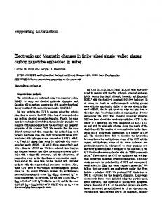
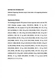
c) Sensitivity Analysis In order assess the robustness of results presented in the paper, Montecarlo analysis was performed on the cultivation of hemp. Results for 1 kg of fiber and woody core are reported in figures 1-3 for mass allocation (fig. 1) and economic allocation (fig. 2,3). When considering mass allocation, results referring to 1 kg of product are the same for fiber and woody core. Results are reported both as percentage (fig. 1a, 2a, 3a), in order to better visualize the error bars, and values (fig. 1b, 2b, 3b), in order to highlight the relative importance of the four contributions of CO2eq. This analysis is significant when taking into account fossil CO2eq and CO2 uptake that are the most important contribution to the total impacts; while CO2eq from land transformation and biogenic holds very low absolute values (see tables 1-2) As it can be observed from the graphics shown in figures 1-3 the error of fossil CO2eq is about 15 % for all the alternatives considered.

Fig. 1a – Montecarlo analysis, mass allocation. Results are reported as %

Woody core / Fiber - Mass allocation 250 200

%

150 100 50

Fossil CO2 eq

Biogenic CO2 eq CO2 eq from land transformation

CO2 uptake

Fig. 1b – Montecarlo analysis, mass allocation. Results are reported as kgCO2eq/kg product

Woody core / Fiber - mass allocation 0.5

0.

kg CO2eq/kg product

Fossil CO2 eq -0.5

-1.

-1.5

-2.

-2.5

Biogenic CO2 eq CO2 eq from land transformation

CO2 uptake

Fig. 2a – Montecarlo analysis, woody core, economic allocation. Results are reported as % woody core - economic allocation 250

200

%

150

100

50

Fossil CO2 eq

Biogenic CO2 eq CO2 eq from land transformation

CO2 uptake

Fig. 2b – Montecarlo analysis, woody core, economic allocation. Results are reported as kgCO2eq/kg product

woody core - economic allocation 0.5 0. kg CO2eq/kg product

Fossil CO2 eq -0.5 -1. -1.5 -2. -2.5

Biogenic CO2 eq CO2 eq from land transformation

CO2 uptake

Fig. 3a – Montecarlo analysis, fiber, economic allocation. Results are reported as %

Fiber - Economic allocation 250

200

%

150

100

50

Fossil CO2 eq

Biogenic CO2 eq CO2 eq from land transformation

CO2 uptake

Fig. 3b – Montecarlo analysis, fiber, economic allocation. Results are reported as kgCO2eq/kg product

Fiber - Economic allocation 0.5

0. Fossil CO2 eq

kg

-0.5

-1.

-1.5

-2.

-2.5

Biogenic CO2 eq CO2 eq from land transformation

CO2 uptake

d) Ecoinvent Database Secondary data taken from Ecoinvent database (www.ecoinvent.ch), one of the world's leading supplier of consistent and transparent life cycle inventory (LCI) data. It is the Swiss center for Life Cycle Inventories and it has combined and extended different LCI databases to provide a set of unified and generic LCI data of high quality. The data are mainly investigated for Swiss and Western European conditions. The Ecoinvent database contains about 4100 datasets of products and services from the energy, transport, building materials, chemicals, pulp and paper, waste treatment and agricultural sector. e) Methods -

Greenhouse Gas Protocol (GGP): developed by the World Resources Institute (WRI) and the World Business Council for Sustainable Development (WBCSD), it is an accounting standard of greenhouse gas emissions. This method is based on the draft report on Product Life Cycle Accounting and Reporting Standard. The total GHG emissions for a product inventory are calculated as the sum of GHG emissions, in CO2eq, of all foreground processes and significant background processes within the system boundary. This method allows for a distinction among: • GHG emissions from fossil sources • Biogenic carbon emissions • Carbon storage • Emissions from land transformation According to the draft standard on product accounting, fossil and biogenic emissions must be reported independently. The reporting of the emissions from carbon storage and land transformation is optional. Reference: WBCSD & WRI (2009) Product Life Cycle Accounting and Reporting Standard. Review Draft for Stakeholder Advisory Group. The Greenhouse Gas Protocol Initiative. November 2009.

-

Cumulative Energy Demand: it allows to calculate the energy consumption of a system and to divide the source of the energy demand (renewable, such as wind power, photovoltaic, hydroelectric, and non-renewable, such as the use of fossil fuels). It also allows to take into account the amount of energy that is stocked in a product (feedstock energy). The feedstock energy is renewable for those products, such as hemp or wood, that actually are renewable resources, while it is a non-renewable fossil for those products such as plastic materials that are made up by non-renewable materials. Characterization factors are given are given for the energy resources divided in 5 impact categories: 1. Non renewable, fossil 2. Non renewable, nuclear 3. Renewable, biomass 4. Renewable, wind, solar, geothermal 5. Renewable, water

In order to get a total (“cumulative”) energy demand, each impact category is given the weighting factor 1. Reference: Frischknecht R., Jungbluth N., et.al. (2003). Implementation of Life Cycle Impact Assessment Methods. Final report ecoinvent 2000, Swiss Centre for LCI. Dübendorf, CH -

Eco-Indicator 99 H: this method converts the results obtained after the characterization step into damage categories, so that eleven impact categories (carcinogens, respiratory organics, respiratory inorganics, climate change, radiation, ozone layer, ecotoxicity, acidification/eutrophication, land use, minerals, fossil fuels) can be grouped and converted into the following damage categories: I. II. III.

Damage to Human Health, expressed as the number of year life lost and the number of years lived disabled. These are combined as Disability Adjusted Life Years (DALYs), Damage to Ecosystem Quality, express as the loss of species over an certain area, during a certain time Damage to Resources, expressed as the surplus energy needed for future extractions of minerals and fossil fuels.

Reference: www.pre-sustainability.com

f)

Thermal transmittance

In order to calculate the thermal transmittance of a wall, we need to define first the global thermal resistance Rtot, expressed as [(m2⋅K)/W]: Rtot= Rsi + ∑(Thicknessi/λi) +Rse Where Thicknessi/λi is the conductivity resistance RCd

Then, the thermal transmittance U, expressed as [W/(m2⋅K)] can be calculated: U=1/Rtot

From data available from table 3 in the manuscript it can be calculated Wall CV.01: Rtot = 5.00 (m2⋅K)/W U = 1/Rtot = 0.200 W/(m2⋅K)

Wall CV.02: Rtot = 5.02 (m2⋅K)/W U = 1/Rtot = 0.199 W/(m2⋅K)