Supporting Information Exploratory machine-learned

Electronic Supplementary Material (ESI) for Chemical Science. This journal is © The Royal Society of Chemistry 2018

Supporting Information

Exploratory machine-learned theoretical chemical shifts can closely predict metabolic mixture signals Kengo Ito,ab Yuka Obuchi,b Eisuke Chikayama,ac Yasuhiro Dateab and Jun Kikuchi*abd a RIKEN b

Center for Sustainable Resource Science, 1-7-22 Suehiro-cho, Tsurumi-ku, Yokohama, Kanagawa 230-0045, Japan.

Graduate School of Medical Life Science, Yokohama City University, 1-7-29 Suehiro-cho, Tsurumi-ku, Yokohama,

Kanagawa 230-0045, Japan. c Department

of Information Systems, Niigata University of International and Information Studies, 3-1-1 Mizukino, Nishi-ku,

Niigata-shi, Niigata 950-2292, Japan. d Graduate

School of Bioagricultural Sciences, Nagoya University, 1 Furo-cho, Chikusa-ku, Nagoya, Aichi 464-0810, Japan.

* Correspondence and requests for materials should be addressed to J.K. (email: [email protected]).

Table of Contents Fig. S1 Analytical flow chart from data collection to the evaluation of predictive modeling ................... 1 Fig. S2 RMSDs between experimental and corrected/uncorrected CSs after QM at the B3LYP/6-31G* level ..... 2 Fig. S3 RMSDs between experimental and corrected/uncorrected CSs after QM at the B3LYP/6-311++G** level .......................................................................................................................................................................... 3 Fig. S4 Average of 10-fold CV RMSDs between experimental and corrected CSs after QM at the B3LYP/6-31G* level …...................................................................................................................................................................... 4 Fig. S5 Average of 10-fold CV RMSDs between experimental and corrected CSs after QM at the B3LYP/6311++G** level ….................................................................................................................................................... 5 Fig. S6 Performance of the ML algorithm xgbLinear for δ1H prediction ……………………………....……...… 6 Fig. S7 Performance of the ML algorithm xgbLinear for δ13C prediction ………..………….……....………..….. 7 Fig. S8 Similarity heat map of the 91 ML algorithms.............................................................................................. 8 Fig. S9 Similarity network diagram of the 91 ML algorithms ................................................................................. 9 Fig. S10 Comparison of conventional δ1H predictive methods with this study’s method using test data ............. 10 Fig. S11 Comparison of conventional δ13C predictive methods with this study’s method using test data ............ 11 Fig. S12 Evaluation of correction effect for theoretical CSs of partial structure ................................................... 12 Fig. S13 Comparison of conventional δ1H predictive methods with this study’s method using 256/402 CSs of test data ......................................................................................................................................................................... 13 Fig. S14 Comparison of conventional δ13C predictive methods with this study’s method using 216/376 CSs of test data .................................................................................................................................................................. 14 Fig. S15 Importance of explanatory variables in the predictive model ................................................................. 15 Fig. S16 Test of the predictive model for HSQC spectral data of C. brachypus extract ...................................... 16 Table S1 List of hyperparameters and their variables..................................................................................... 17 Table S2 List of RMSDs between experimental and theoretical/predicted CSs of metabolites in C. brachypus ................................................................................................................................................. 21 Table S3 List of the 150 compounds used as a training data set for modeling ..................................................... 22 Table S4 List of 34 compounds included in the test data set ................................................................................. 25 Table S5 List of the objective and explanatory variables ….................................................................................. 26 Table S6 Part of the data set for ML ...................................................................................................................... 27 Table S7 List of the 91 ML algorithms ................................................................................................................. 28 Table S8 List of model types or relevant characteristics of the ML algorithms …................................................ 30

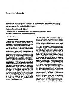
Fig. S1 Analytical flow chart from data collection to the evaluation of predictive modeling (A), and test of predictive model using test data set (B). First, PubChem compound identifications (CIDs) of 150 compounds that we used as standard substances (Table S3) were listed as “metid_list.txt” (1), and searched at the PubChem website (https://pubchem.ncbi.nlm.nih.gov/) (2) to obtain 3D structure files (3). The structure file format was converted from SDF (3) to XYZ (4) using openbabel software. To calculate theoretical NMR parameters, the XYZ file was converted to a Gaussian09 command file by shell script (5-6); a log file including theoretical CS and J value was also obtained at this time (7). Experimental NMR spectra of the 150 compounds were assigned by using databases (8-9). CID, atom number, solvent number, experimental CS, and theoretical shielding constant of each reference substance (e.g., tetramethylsilane) were saved as “experiment_database.txt” (10). Training data sets (“metid_list.txt_H.txt” and “metid_list.txt_C.txt”) (Table S5 and S6) were generated by the Java program “toolgaussianlearndata.jar” from “metid_list.txt”, “experiment_database.txt”, “CID.sdf” and “CID.log” (11). In total, 91 ML algorithms (Table S7) (12) and their hyperparameters (Table S1) (13) were explored to identify the best predictive model. At this time, 10-fold CV was calculated to evaluate over-learning and overfitting (14-18). After the 3-grid search, the final model with the lowest RMSD was exported (19), and the importance of explanatory variables was calculated. Lastly, the predictive models, RMSDs, and importance of 91 MLs were saved as Rdata (21). The steps of ML (12-21) were calculated automatically by using the R program “Several_Predictive_Modeling_for_QM.R”, which depends on the caret library (https://topepo.github.io/caret/). A total of 34 compounds which does not include learning and k-fold validation (training) data sets of ML (Table S4), and seaweed components were used as the test data set (22). Collection of structure files (23), QM calculations (24), and collection of experimental CS (25) were performed in same way using steps (2-10). Test data sets were also generated (26) in the same way using step (11). CSs of test data sets were predicted by the learned predictive model using the R program “Applying_Model.R” (27). Finally, predicted CSs were compared with experimental CSs (28), and the predictive accuracy was determined by RMSDs (29). Example data and programs for generating the data set for ML from experimental/theoretical data, and the 91 MLs with the grid search CV approach used in this study are deposited on our website (http://dmar.riken.jp/Rscripts/).

1

B

Machine Learning Algorithms

randomGLM ANFIS DENFIS rbf DDA mlp QM (Non corr.) mlpML superpc mlpWeightDecay ML rf Rules mlpSGD mlpWeightDecay dnn krlsPoly elm pcr rbf leapForward leapSeq icr rqnc leapBackward widekernelpls simpls pls kernelpls relaxo glmnet nnls BstLm rqlasso glmboost sv mLinear3 partDSA plsRglm blasso ctree2 lars2 penalized gaussprLinear sv mLinear2 sv mLinear bridge rv mLinear blassoAv eraged lmStepAIC glmStepAIC lasso bay esglm enet f oba lm lars glm nodeHarv est earth nnet gcv Earth ev tree av NNet pcaNNet bagEarth gaussprRadial rv mRadial cf orest bagEarthGCV ppr ctree rv mPoly qrf knn gbm brnn sv mPoly sv mRadialCost sv mRadial WM sv mRadialSigma krlsRadial gaussprPoly SBC kknn bartMachine Rborist cubist parRF RRFglobal RRF rf xgbTree extraTrees xgbLinear

0.0

0.1

0.2

0.3

～ ～

～ ～

Machine Learning Algorithms

A

randomGLM ANFIS DENFIS rf Rules mlpML mlpSGD rbf DDA mlpWeightDecay ML QM (Non corr.) mlpWeightDecay mlp dnn av NNet nnet pcaNNet rbf krlsPoly superpc leapSeq leapBackward relaxo elm icr leapForward pcr nnls partDSA widekernelpls simpls pls kernelpls BstLm sv mLinear3 rv mLinear glmboost ctree2 plsRglm nodeHarv est lars2 rqnc rqlasso sv mLinear sv mLinear2 lars blasso bridge blassoAv eraged penalized earth gcv Earth bagEarth ctree glmnet lmStepAIC glmStepAIC gaussprLinear lasso bay esglm f oba enet lm glm bagEarthGCV cf orest ev tree gaussprPoly gaussprRadial qrf knn sv mPoly gbm WM sv mRadialSigma sv mRadial sv mRadialCost brnn rv mPoly ppr rv mRadial krlsRadial SBC bartMachine Rborist cubist xgbTree RRF RRFglobal parRF rf extraTrees kknn xgbLinear

0

0.4

RMSD (δ1H) [ppm]

2

4

6

8

10

RMSD (δ13C) [ppm]

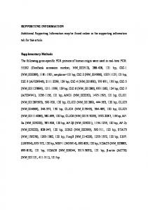
Fig. S2 RMSDs between experimental and theoretical (red)/predicted (black) CSs of 150 compounds as training data set. (A) δ1H and (B) δ13C were corrected by 91 ML algorithms after QM at the B3LYP/6-31G* level. These figures are expanded versions of Fig. 1B. These RMSDs indicate learning errors. The dotted line indicates the RMSD (δ1H=0.2442 ppm, δ13C=3.7513 ppm) of the predicted CSs of 150 compounds calculated by Mnova; the unbroken line indicates the recommended tolerances (δ1H=0.03 ppm, δ13C=0.53 ppm) for assignment from the SpinAssign tool.

2

B

Machine Learning Algorithms

randomGLM ANFIS DENFIS mlpSGD mlp rf Rules rbf DDA QM (Non corr.) mlpWeightDecay mlpWeightDecay ML mlpML dnn krlsPoly rbf pcr nnls icr superpc elm leapBackward leapSeq leapForward rqnc nnet pcaNNet enet av NNet widekernelpls simpls pls kernelpls partDSA BstLm rv mLinear glmboost plsRglm relaxo ctree2 sv mLinear3 penalized rqlasso lars2 sv mLinear2 gaussprLinear blasso bridge sv mLinear blassoAv eraged nodeHarv est lmStepAIC glmStepAIC glmnet lasso bay esglm f oba lars lm glm rv mPoly earth ev tree gcv Earth bagEarth gaussprRadial bagEarthGCV cf orest rv mRadial qrf gbm ppr knn sv mRadialCost sv mRadial ctree brnn sv mPoly krlsRadial WM sv mRadialSigma SBC kknn bartMachine gaussprPoly Rborist cubist parRF RRF rf RRFglobal xgbTree extraTrees xgbLinear

0.0

0.1

0.2

0.3

0.4

～ ～

～ ～

Machine Learning Algorithms

A

ANFIS randomGLM DENFIS rf Rules rbf DDA av NNet QM (Non corr.) nnet elm pcaNNet mlpSGD superpc mlpWeightDecay ML mlpWeightDecay mlpML nnls dnn mlp krlsPoly rbf leapForward icr leapBackward pcr leapSeq partDSA widekernelpls simpls pls kernelpls sv mLinear3 relaxo ctree2 BstLm glmboost plsRglm nodeHarv est earth gcv Earth rv mLinear rqnc lars2 rqlasso bagEarth lasso sv mLinear2 sv mLinear blasso bridge cf orest blassoAv eraged penalized lmStepAIC glmStepAIC gaussprLinear glmnet bay esglm enet f oba lars lm glm bagEarthGCV ctree ev tree sv mPoly gaussprPoly rv mPoly sv mRadial sv mRadialCost qrf gaussprRadial knn gbm sv mRadialSigma ppr WM brnn bartMachine SBC krlsRadial rv mRadial Rborist cubist rf RRFglobal parRF RRF extraTrees xgbTree xgbLinear kknn

0

RMSD (δ1H) [ppm]

2

4

6

8

10

RMSD (δ13C) [ppm]

Fig. S3 RMSDs between experimental and theoretical (red)/predicted (black) CSs of 150 compounds as a training data set. (A) δ1H and (B) δ13C were corrected by 91 ML algorithms after QM at the B3LYP/6-311++G** level. These RMSDs indicate learning errors. The dotted line indicates the RMSDs (δ1H=0.2442 ppm, δ13C=3.7513 ppm) of predicted CSs of 150 compounds calculated by Mnova; the unbroken line indicates the recommended tolerances (δ1H=0.03 ppm, δ13C=0.53 ppm) for assignment from the SpinAssign tool.

3

B

Machine Learning Algorithms

randomGLM ANFIS DENFIS rbf DDA mlpML rf Rules mlp mlpSGD superpc mlpWeightDecay ML mlpWeightDecay dnn krlsPoly pcr leapForward leapSeq elm icr rqnc leapBackward rbf widekernelpls pls kernelpls simpls relaxo sv mLinear3 WM glmnet rqlasso BstLm rv mLinear nnls glmboost plsRglm partDSA SBC qrf ctree2 lmStepAIC sv mLinear penalized lars2 gaussprLinear sv mLinear2 glmStepAIC blasso lm lars glm bridge bay esglm blassoAv eraged enet f oba nodeHarv est lasso ev tree earth nnet av NNet rv mRadial pcaNNet ctree gcv Earth gaussprRadial knn bagEarth cf orest ppr rv mPoly kknn brnn sv mRadialCost gbm bagEarthGCV sv mRadial sv mPoly sv mRadialSigma krlsRadial gaussprPoly bartMachine xgbTree Rborist RRF rf RRFglobal cubist parRF xgbLinear extraTrees

0.0

0.1

0.2

0.3

randomGLM ANFIS glm DENFIS rf Rules rbf DDA mlpSGD mlpML mlp mlpWeightDecay ML mlpWeightDecay nnet av NNet pcaNNet dnn rbf krlsPoly superpc leapSeq leapBackward relaxo icr elm nnls leapForward pcr WM partDSA widekernelpls pls kernelpls simpls BstLm ctree2 sv mLinear3 plsRglm glmboost rv mLinear qrf ctree earth lars2 gcv Earth SBC rqnc enet sv mLinear rqlasso nodeHarv est sv mLinear2 lars penalized gaussprLinear blasso glmStepAIC f oba lasso sv mRadialSigma bagEarth glmnet bay esglm cf orest rv mRadial lm lmStepAIC bagEarthGCV sv mRadial blassoAv eraged gaussprRadial bridge rv mPoly ev tree ppr sv mRadialCost gaussprPoly knn brnn sv mPoly gbm kknn krlsRadial bartMachine parRF xgbTree Rborist RRFglobal rf extraTrees cubist RRF xgbLinear

～ ～

～ ～

Machine Learning Algorithms

A

0

0.4

10 Fold CV RMSD (δ1H) [ppm]

2

4

6

8

10

10 Fold CV RMSD (δ13C) [ppm]

Fig. S4 10-fold CV RMSDs between experimental and predicted CSs of 150 compounds as a training data set. (A) δ1H and (B) δ13C were corrected by 91 ML algorithms after QM at the B3LYP/6-31G* level. These RMSDs indicate generalization errors.

4

B

Machine Learning Algorithms

randomGLM ANFIS DENFIS rf Rules mlpSGD mlp rbf DDA mlpML mlpWeightDecay dnn mlpWeightDecay ML krlsPoly pcr nnls icr elm superpc leapBackward leapSeq leapForward pcaNNet rqnc nnet av NNet simpls kernelpls widekernelpls enet pls rbf partDSA WM SBC BstLm ctree2 plsRglm glmboost relaxo qrf sv mLinear3 rv mLinear penalized lars2 gaussprLinear sv mLinear rqlasso ev tree bridge blasso lm sv mLinear2 glm nodeHarv est glmStepAIC blassoAv eraged lars lmStepAIC bay esglm lasso f oba glmnet knn rv mRadial earth gaussprRadial gcv Earth kknn bagEarth cf orest bagEarthGCV rv mPoly ctree sv mRadialCost sv mRadial ppr gbm brnn krlsRadial sv mPoly sv mRadialSigma gaussprPoly bartMachine xgbTree extraTrees Rborist cubist RRFglobal parRF RRF xgbLinear rf

0.0

0.1

0.2

0.3

～ ～

～ ～

Machine Learning Algorithms

A

randomGLM ANFIS DENFIS rf Rules rbf DDA av NNet pcaNNet nnet superpc mlpSGD elm nnls mlpML mlpWeightDecay ML mlp mlpWeightDecay krlsPoly dnn leapForward rbf icr leapBackward pcr relaxo leapSeq WM partDSA kernelpls widekernelpls pls simpls ctree2 bagEarthGCV sv mLinear3 BstLm glmboost qrf plsRglm lm nodeHarv est rv mLinear earth ctree SBC gcv Earth ev tree rqnc bagEarth sv mLinear2 lars2 penalized cf orest sv mLinear lasso enet bridge lmStepAIC glm glmStepAIC glmnet f oba bay esglm gaussprLinear blasso lars blassoAv eraged sv mRadialCost sv mRadial rqlasso rv mPoly gaussprRadial sv mPoly rv mRadial sv mRadialSigma knn ppr gaussprPoly kknn brnn gbm krlsRadial bartMachine RRFglobal Rborist xgbTree cubist RRF extraTrees xgbLinear parRF rf

0

0.4

10 Fold CV RMSD (δ1H) [ppm]

2

4

6

8

10

10 Fold CV RMSD (δ13C) [ppm]

Fig. S5 10-fold CV RMSDs between experimental and predicted CSs of 150 compounds as a training data set. (A) δ1H and (B) δ13C were corrected by 91 ML algorithms after QM at the B3LYP/6-311++G** level. These RMSDs indicate generalization errors.

5

5

6 7

8

9 10 11

13

15

17

19 20 21

23

25

27

1.0 0.8 0.6 0.4 0.2

3 4

0

1 2

B Absolute error [ppm]

R squared

0.790 0.79 0.785 0

Grid1 * Grid1 * Grid1 Grid1 * Grid2 * Grid1 Grid1 * Grid3 * Grid3 Grid1 * Grid1 * Grid2 Grid1 * Grid3 * Grid2 Grid1 * Grid2 * Grid2 Grid1 * Grid3 * Grid1 Grid3 * Grid1 * Grid1 Grid2 * Grid1 * Grid1 Grid2 * Grid3 * Grid2 Grid2 * Grid1 * Grid2 Grid2 * Grid2 * Grid1 Grid3 * Grid1 * Grid2 Grid3 * Grid2 * Grid1 Grid2 * Grid2 * Grid2 Grid3 * Grid3 * Grid2 Grid3 * Grid2 * Grid2 Grid2 * Grid3 * Grid1 Grid3 * Grid3 * Grid1 Grid1 * Grid2 * Grid3 Grid1 * Grid1 * Grid3 Grid2 * Grid3 * Grid3 Grid3 * Grid3 * Grid3 Grid2 * Grid1 * Grid3 Grid2 * Grid2 * Grid3 Grid3 * Grid1 * Grid3 Grid3 * Grid2 * Grid3

0.775

0.140

0.140

0.780 0.78

0.142

RMSD

0.144 0.144

0.795

0.146

0.800 0.80

A

1 2 3 4 5 6 7 8 9 10

Grid combination [nrounds * lambda * alpha]

Fold No.

C Fold No. Fold 01 Fold 02 Fold 03 Fold 04 Fold 05 Fold 06 Fold 07 Fold 08 Fold 09 Fold 10

Abs. Min. 0.000454 0.000160 0.000090 0.000244 0.000168 0.000421 0.000076 0.000296 0.000882 0.001049

Abs. 1st Qu. Abs. Median 0.009740 0.039180 0.012360 0.039170 0.011320 0.039480 0.008496 0.029740 0.011530 0.032990 0.011440 0.041270 0.008431 0.039100 0.013390 0.043630 0.013670 0.037990 0.012610 0.043010

Abs. Mean Abs. 3rd Qu. Abs. Max. 0.081840 0.103800 0.940100 0.093210 0.095120 0.744600 0.083750 0.096810 0.749900 0.070550 0.090130 0.502800 0.075980 0.085930 0.624000 0.077440 0.106700 0.518600 0.069430 0.073400 0.547100 0.075470 0.087010 0.932300 0.070390 0.080540 0.718500 0.083940 0.097080 0.793600

Variance 0.08876628 0.08045715 0.09273747 0.08376600 0.06856733 0.07560452 0.06987863 0.06642588 0.08310468 0.09211333

Fig. S6 Performance of the ML algorithm xgbLinear for δ1H prediction. Theoretical CSs were calculated at the B3LYP/631G*//GIAO/B3LYP/6-31G* level. (A) Convergence curve of hyperparameters determined by the grid search for a combination of 3 hyperparameters (nrounds=50 [Grid1], 100 [Grid2], 150 [Grid3]; lambda=0 [Grid1], 0.0001 [Grid2], 0.1 [Grid3]; alpha=0 [Grid1], 0.0001 [Grid2], 0.1 [Grid3]). The right-most (green) grid combination is the best model, having the lowest RMSD (red) with highest R2 (blue). The hyperparameters nrounds=150, lambda=0.0001, and alpha=0.1 were selected and used for the final CS prediction. Other hyperparameters are shown in Table S1. (B) Absolute errors between experimental CS and predicted CS for the validation set were calculated by using 10-fold CV to evaluate over-learning and over-fitting. Boxplots show absolute errors of 128 CSs (dot) in each fold. The 128 CSs in the validation set were calculated by using a predictive model, which was learned by using 1149 CSs as a learning set. The statistics (absolute minimum error, absolute 1st quarter error, absolute median error, absolute mean error, absolute 1st quarter error, absolute maximum error, and variance) are shown in (C).

6

0.893 1 2

3 4

5

6 7

8

9 10 11

13

15

17

19 20 21

23

25

27

Grid combination [nrounds * lambda * alpha]

0

0

Grid1 * Grid3 * Grid2 Grid3 * Grid3 * Grid2 Grid2 * Grid3 * Grid2 Grid1 * Grid1 * Grid2 Grid1 * Grid1 * Grid1 Grid3 * Grid1 * Grid1 Grid1 * Grid3 * Grid1 Grid3 * Grid3 * Grid1 Grid3 * Grid1 * Grid2 Grid1 * Grid2 * Grid1 Grid2 * Grid3 * Grid1 Grid2 * Grid1 * Grid1 Grid1 * Grid3 * Grid3 Grid2 * Grid1 * Grid2 Grid3 * Grid3 * Grid3 Grid1 * Grid2 * Grid2 Grid2 * Grid3 * Grid3 Grid1 * Grid1 * Grid3 Grid3 * Grid2 * Grid1 Grid3 * Grid2 * Grid2 Grid2 * Grid2 * Grid1 Grid2 * Grid2 * Grid2 Grid3 * Grid2 * Grid3 Grid1 * Grid2 * Grid3 Grid3 * Grid1 * Grid3 Grid2 * Grid2 * Grid3 Grid2 * Grid1 * Grid3

5

10

Absolute error [ppm]

R squared

0.896 0.896 0.894 0.894

0.895

2.2152.220

RMSD

2.210

2.200 2.20

15

B

2.230 2.23

A

1 2 3 4 5 6 7 8 9 10

Fold No.

C Fold No. Fold 01 Fold 02 Fold 03 Fold 04 Fold 05 Fold 06 Fold 07 Fold 08 Fold 09 Fold 10

Abs. Min. 0.001844 0.001257 0.000682 0.007560 0.014230 0.017980 0.002369 0.003957 0.002760 0.006155

Abs. 1st Qu. Abs. Median Abs. Mean Abs. 3rd Qu. Abs. Max. 0.2538 0.5908 1.218 1.432 9.23 0.2222 0.6193 1.357 1.480 11.03 0.2324 0.5861 1.302 1.379 11.33 0.1869 0.5726 1.143 1.139 11.51 0.1671 0.5155 1.266 1.642 10.90 0.2731 0.5510 1.319 1.268 14.32 0.3146 0.6607 1.185 1.352 9.63 0.2208 0.4688 1.186 1.282 12.23 0.2201 0.7032 1.155 1.550 5.54 0.2991 0.6255 1.505 2.158 10.52

Variance 40.42158 40.91832 44.07397 45.60710 45.35547 43.18276 45.57893 36.51587 41.90630 39.61191

Fig. S7 Performance of the ML algorithm xgbLinear for δ13C prediction. Theoretical CSs were calculated at the B3LYP/631G*//GIAO/B3LYP/6-31G* level. (A) Convergence curve of hyperparameters determined by the grid search for a combination of 3 hyperparameters (nrounds=50 [Grid1], 100 [Grid2], 150 [Grid3]; lambda=0 [Grid1], 0.0001 [Grid2], 0.1 [Grid3]; alpha=0 [Grid1], 0.0001 [Grid2], 0.1 [Grid3]). The right-most grid combination (green) is the best model, having the lowest RMSD (red) with highest R2 (blue). The hyperparameters nrounds=100, lambda=0, and alpha=0.1 were selected and used for the final CS prediction. Other hyperparameters are shown in Table S1. (B) Absolute errors between experimental CS and predicted CS for the validation set were calculated by using 10-fold cross validation to evaluate overlearning and over-fitting. Boxplots show absolute errors of 108 CSs (dot) in each fold. The 108 CSs in the validation set were calculated by using a predictive model, which was learned by using 970 CSs as a learning set. The statistics (absolute minimum error, absolute 1st quarter error, absolute median error, absolute mean error, absolute 1st quarter error, absolute maximum error, and variance) are shown in (C).

7

Jaccard Coefficient

1

75 68 70 34 47 39 32 67 74 69 73 40 46 45 72 48 52 53 54 49 33 36 25 29 30 42 88 6 7 10 5 3 4 61 9 1 11 55 8 22 43 44 57 28 41 80 78 79 87 82 71 81 77 85 86 83 84 17 15 90 89 12 21 76 13 59 16 14 60 50 51 23 18 19 20 65 64 62 63 56 91 35 58 31 38 37 27 26 66 2 24

24 2 66 26 27 37 38 31 58 35 91 56 63 62 64 65 20 19 18 23 51 50 60 14 16 59 13 76 21 12 89 90 15 17 84 83 86 85 77 81 71 82 87 79 78 80 41 28 57 44 43 22 8 55 11 1 9 61 4 3 5 10 7 6 88 42 30 29 25 36 33 49 54 53 52 48 72 45 46 40 73 69 74 67 32 39 47 34 70 68 75

ML algorithm No.

0

ML algorithm No. Fig. S8 Heat map showing the similarity among the 91 ML algorithms. The color indicates the Jaccard coefficient, with darker color indicating more similar models. The numbers correspond to the algorithms listed in Table S7.

8

good

1

bad

91

Fig. S9 Network diagram showing clusters of similar model types or relevant characteristics of the 91 ML algorithms. The numbers correspond to the algorithms listed in Table S7. The nodes are connected by Jaccard similarity (>0.56). Node colors indicate the performance of the δ13C predictive model (Fig. S2B): good models show low RMSDs; poor models show high RMSDs.

9

4

6

8

0

2

δ1H

4

6

8

10

(Expt.) [ppm]

10 8 6 4 2

0

2

δ1H

4

6

8

10

(Expt.) [ppm]

6 4 2

RMSD = 0.2080 0

2

δ1H

4

6

8

10

(Expt.) [ppm]

NMRShiftDB

8

10

F QM1’ + ML

8

10

0

10

(Expt.) [ppm]

0

δ1H (Pred.) [ppm]

6 4 0

2

RMSD = 0.3593

δ1H (Pred.) [ppm]

10 8 6 4

2

δ1H

E QM1’

8

10

0

(Expt.) [ppm]

D δ1H (Pred.) [ppm]

2

10

6

8

4

6

RMSD = 0.2271

RMSD = 0.3329

2

4

RMSD = 0.2177

Mnova

0

2

δ1H

QM1+ML

δ1H (Pred.) [ppm]

0

C

0

6 4 2

RMSD = 0.3136

δ1H (Pred.) [ppm]

QM1

8

10

B

0

δ1H (Pred.) [ppm]

A

0

2

δ1H

4

6

8

10

(Expt.) [ppm]

10 4

6

8

QM2

2

RMSD = 0.3501

0

δ1H (Pred.) [ppm]

G

0

2

δ1H

4

6

8

10

(Expt.) [ppm]

Fig. S10 Comparison of conventional prediction methods based on (A, D, G) quantum chemistry and (C, F) a data-driven approach with (B, E) this study’s method. This figure is an expanded version of Fig. 2 with the addition of different calculation levels employed in Gaussian09 software (D), QM1’ with ML predictive approach (E), NMRShiftDB (F), and Spartan (G) results. Experimental CSs are compared with the calculated δ1H of 34 compounds in D2O and MeOD solvent as test data set (Table 4). In total, 402 CSs of test data set were plotted for δ1H. QM1 shows the theoretical CSs calculated at the B3LYP/6-31G*//GIAO/B3LYP/6-31G* level, and QM1’ shows the theoretical CSs calculated at the B3LYP/6311++G**//GIAO/B3LYP/6-311++G** level using Gaussian09 software. QM1+ML and QM1’+ML show the results of the predictive approach described in this study, in which the ML algorithm xgbLinear calculates an SF that is applied to QM1 and QM1’. QM2 shows the theoretical CSs calculated at the EDF2/6-31G* level using Spartan’14 software. The theoretical CSs of QM2 were corrected with the weighted average using a Boltzmann distribution after conformational analysis.

10

100

150

0

50

δ13C

100

150

200

(Expt.) [ppm]

200 150 100 50 0

50

δ13C

100

150

200

(Expt.) [ppm]

F

100 50

RMSD = 3.4687 0

50

δ13C

100

150

200

(Expt.) [ppm]

200

NMRShiftDB

150

QM1’ + ML

150

200

0

200

(Expt.) [ppm]

0

δ13C (Pred.) [ppm]

100 50 0

RMSD = 7.2527

δ13C (Pred.) [ppm]

200 150 100

50

δ13C

E QM1’

150

200

0

(Expt.) [ppm]

D δ13C (Pred.) [ppm]

50

200

100

150

RMSD = 3.7600

50

100

RMSD = 3.3261

Mnova

RMSD = 4.5730

0

50

δ13C

QM1+ML

δ13C (Pred.) [ppm]

0

C

0

100 50

RMSD = 7.4477

δ13C (Pred.) [ppm]

QM1

150

200

B

0

δ13C (Pred.) [ppm]

A

0

50

δ13C

100

150

200

(Expt.) [ppm]

200 50

100

150

QM2

RMSD = 5.0681

0

δ13C (Pred.) [ppm]

G

0

50

100

150

200

δ13C (Expt.) [ppm] Fig. S11 Comparison of conventional prediction methods based on (A, D, G) quantum chemistry and (C, F) a data-driven approach with (B, E) this study’s method. This figure is an expanded version of Fig. 2 with the addition of different calculation level using Gaussian09 software (D), QM1’ with ML predictive approach (E), NMRShiftDB (F), and Spartan (G) results. Experimental CSs are compared with the calculated δ13C of 34 compounds in D2O and MeOD solvent as test data set (Table S4). In total, 376 CSs of test data set were plotted for δ13C. QM1 shows the theoretical CSs calculated at the B3LYP/6-31G*//GIAO/B3LYP/6-31G* level, and QM1’ shows the theoretical CSs calculated at the B3LYP/6311++G**//GIAO/B3LYP/6-311++G** level using Gaussian09 software. QM1+ML and QM1’+ML show the results of the predictive approach described in this study, in which the ML algorithm xgbLinear calculates an SF that is applied to QM1 and QM1’. QM2 shows the theoretical CSs calculated at the EDF2/6-31G* level using Spartan’14 software. The theoretical CSs of QM2 were corrected with the weighted average using a Boltzmann distribution after conformational analysis.

11

10 8 6 4 2

10C

9C

8C

7C

6C

5C 10

QM

2

4

6

8

QM+ML

10

10C

7C

6C

0

Error of δ13C [ppm]

QM

4

6

8

QM+ML

10C

6C 10 2

4

6

8

QM+ML

12C

11C

10C

9C

8C

7C

5C 10

QM

2

4

6

8

QM+ML

Atom No.

9C

8C

7C

6C

5C

12H 13H 14H 15H 16H 17H 18H 19H 20H 21H

0

Error of δ13C [ppm]

QM+ML

QM

0

Error of δ13C [ppm]

22H

21H

20H

18H 19H

17H

14H 15H

13H

QM

8C

0 14H

13H

12H

0.4

0.6

0.8

QM+ML

0.2 0.0 1.0

QM+ML

2

0.6 0.4 0.2 0.0

QM

0.6

0.8

Error of δ13C [ppm]

17H

15H

16H 15_16_17H

13H

QM+ML

0.4

Error of δ1H [ppm]

12H

11H

QM

0.8

1.0

0.0

0.2

0.4

0.6

QM+ML

0.2 0.0

Pimelate

Error of δ1H [ppm]

Tryptamine

QM

0 11H 12H 13H 14H 15H 16H 17H 18H 19H 20H 21H 22H

QM

0.8

1.0

0.0

0.2

0.4

0.6

QM+ML

Error of δ13C [ppm]

0.8

QM

1.0

3,4-Dihydroxybenzoate

Error of δ1H [ppm]

N-Acetyl-DL-cysteine

Error of δ1H [ppm]

Triethanolamine

C 1.0

B Error of δ1H [ppm]

A

Atom No.

Fig. S12 Evaluation of correction effect for theoretical CSs of partial structure. Five compounds in test set and its atom number are shown as examples (A). The errors of δ1H (B) and δ13C (C) between experimental CS and predicted CS of each atoms are plotted. QM (black bar) shows the errors of theoretical CSs calculated at the B3LYP/6-31G*//GIAO/B3LYP/631G* level, and QM+ML (gray bar) shows the errors of predicted CSs using the predictive approach described in this study.

12

4

6

8

0

2

δ1H

4

6

8

10

(Expt.) [ppm]

10 8 6 4 2

0

2

δ1H

4

6

8

10

(Expt.) [ppm]

6 4 2

RMSD = 0.1223 0

2

δ1H

4

6

8

10

(Expt.) [ppm]

NMRShiftDB

8

10

F QM1’ + ML

8

10

0

10

(Expt.) [ppm]

0

δ1H (Pred.) [ppm]

6 4 0

2

RMSD = 0.2805

δ1H (Pred.) [ppm]

10 8 6 4

2

δ1H

E QM1’

8

10

0

(Expt.) [ppm]

D δ1H (Pred.) [ppm]

2

10

6

8

4

6

RMSD = 0.1706

RMSD = 0.3280

2

4

RMSD = 0.0800

Mnova

0

2

δ1H

QM1+ML

δ1H (Pred.) [ppm]

0

C

0

6 4 2

RMSD = 0.2372

δ1H (Pred.) [ppm]

QM1

8

10

B

0

δ1H (Pred.) [ppm]

A

0

2

δ1H

4

6

8

10

(Expt.) [ppm]

10 4

6

8

QM2

2

RMSD = 0.3095

0

δ1H (Pred.) [ppm]

G

0

2

δ1H

4

6

8

10

(Expt.) [ppm]

Fig. S13 Comparison of conventional prediction methods based on (A, D, G) quantum chemistry and (C, F) a data-driven approach with (B, E) this study’s method. This figure is an expanded version of Fig. 3 with the addition of different calculation level using Gaussian09 software (D), QM1’ with ML predictive approach (E), NMRShiftDB (F), and Spartan (G) results. Experimental CSs are compared with the calculated δ1H of 34 compounds in D2O and MeOD solvent as test data set (Table S4). In total, 256 CSs in 402 CSs of test data set were plotted for δ1H. These CSs of partial structure were well learned. QM1 shows the theoretical CSs calculated at the B3LYP/6-31G*//GIAO/B3LYP/6-31G* level, and QM1’ shows the theoretical CSs calculated at the B3LYP/6-311++G**//GIAO/B3LYP/6-311++G** level using Gaussian09 software. QM1+ML and QM1’+ML show the results of the predictive approach described in this study, in which the ML algorithm xgbLinear calculates an SF that is applied to QM1 and QM1’. QM2 shows the theoretical CSs calculated at the EDF2/631G* level using Spartan’14 software. The theoretical CSs of QM2 were corrected with the weighted average using a Boltzmann distribution after conformational analysis.

13

δ13C (Expt.) [ppm]

150

0

50

δ13C

100

150

200

(Expt.) [ppm]

50

100

200 150 100 50 0

100

150

200

δ13C (Expt.) [ppm]

RMSD = 2.1882 0

50

δ13C

100

150

200

(Expt.) [ppm]

200

NMRShiftDB

150

150

200

50

F QM1’ + ML

0

RMSD = 6.5941

0

200

δ13C (Expt.) [ppm]

δ13C (Pred.) [ppm]

50

100

150

200

100

E QM1’

0

δ13C (Pred.) [ppm]

D

50

δ13C (Pred.) [ppm]

200 150 100 50

0

200

100

150

RMSD = 3.5215

50

100

RMSD = 0.9798

Mnova

RMSD = 4.0771

0

50

QM1+ML

δ13C (Pred.) [ppm]

0

C

0

100 50

RMSD = 7.6091

δ13C (Pred.) [ppm]

QM1

150

200

B

0

δ13C (Pred.) [ppm]

A

0

50

δ13C

100

150

200

(Expt.) [ppm]

200 50

100

150

QM2

RMSD = 5.1113

0

δ13C (Pred.) [ppm]

G

0

50

100

150

200

δ13C (Expt.) [ppm] Fig. S14 Comparison of conventional prediction methods based on (A, D, G) quantum chemistry and (C, F) a data-driven approach with (B, E) this study’s method. This figure is an expanded version of Fig. 3 with the addition of different calculation level using Gaussian09 software (D), QM1’ with ML predictive approach (E), NMRShiftDB (F), and Spartan (G) results. Experimental CSs are compared with the calculated δ13C of 34 compounds in D2O and MeOD solvent as test data set (Table S4). In total, 216 CSs in 376 CSs of test data set were plotted for δ13C. These CSs of partial structure were well learned. QM1 shows the theoretical CSs calculated at the B3LYP/6-31G*//GIAO/B3LYP/6-31G* level, and QM1’ shows the theoretical CSs calculated at the B3LYP/6-311++G**//GIAO/B3LYP/6-311++G** level using Gaussian09 software. QM1+ML and QM1’+ML show the results of the predictive approach described in this study, in which the ML algorithm xgbLinear calculates an SF that is applied to QM1 and QM1’. QM2 shows the theoretical CSs calculated at the EDF2/6-31G* level using Spartan’14 software. The theoretical CSs of QM2 were corrected with the weighted average using a Boltzmann distribution after conformational analysis.

14

A

B

3J OH 3J HH 3J HH 3J CH

(4th) [Hz] 3J(O)_4 th) [Hz] (8 3J(H)_8 th) [Hz] (7 3J(H)_7 th) [Hz] (4 3J(C)_4 H-X-P [n] BondedBonded(P) H-X-H [n] BondedBonded(H) H-C [n] Bonded(C) 3J st (1 ) [Hz] PH3J(P)_1 2J (1st) [Hz] PH2J(P)_1 2J (2nd) [Hz] OH2J(O)_2 H-X-S [n] BondedBonded(S) 2J (3rd) [Hz] CH2J(C)_3 3J (6th) [Hz] HH3J(H)_6 3J (1st) [Hz] SH3J(S)_1 3J (3rd) [Hz] OH3J(O)_3 Aromatic (C) [Y/N] Aromatic(C) H-X-N [n] BondedBonded(N) 3J (3rd) [Hz] NH3J(N)_3 2J (2nd) [Hz] NH2J(N)_2 Aromatic (N) [Y/N] Aromatic(N) H-X-O [n] BondedBonded(O) 2J (2nd) [Hz] HH2J(H)_2 C/CH/CH C/CH/CH2/CH3/CH4 2/CH3/CH4 [type] 3J (5th) [Hz] HH3J(H)_5 3J (3rd) [Hz] HH3J(H)_3 Solvent [type] Solvent H-X-C [n] BondedBonded(C) 3J (4th) [Hz] HH3J(H)_4 2J (1st) [Hz] OH2J(O)_1 3J (2nd) [Hz] HH3J(H)_2 3J (3rd) [Hz] CH3J(C)_3 2J (1st) [Hz] SH2J(S)_1 2J (1st) [Hz] HH2J(H)_1 3J nd) [Hz] (2 OH3J(O)_2 2J nd) [Hz] (2 CH2J(C)_2 3J (2nd) [Hz] NH3J(N)_2 3J (1st) [Hz] HH3J(H)_1 3J (1st) [Hz] OH3J(O)_1 2J (1st) [Hz] CH2J(C)_1 3J (2nd) [Hz] CH3J(C)_2 1J (1st) [Hz] CH1J(C)_1 3J (1st) [Hz] CH3J(C)_1 CS [ppm] Chemical shift(theor)(ppm) 3J (1st) [Hz] NH3J(N)_1 2J (1st) [Hz] NH2J(N)_1

3J

(1 ) [Hz] 3J(S)_1 (3rd) [Hz] 3J(N)_3 3J (10th) [Hz] CH 3J(H)_10 3J (9th) [Hz] CN 3J(H)_9 2J (4th) [Hz] CN 2J(N)_4 2J (3rd) [Hz] CN 2J(N)_3 2J (4th) [Hz] CO 2J(O)_4 2J (4th) [Hz] CC 2J(C)_4 1J (1st) [Hz] CS 1J(S)_1 Aromatic (N) [Y/N] Aromatic(N) C-P [n] Bonded(P) C-H [n] Bonded(H) 2J (1st) [Hz] CP 2J(P)_1 1J (3rd) [Hz] CN 1J(N)_3 1J (1st) [Hz] CP 1J(P)_1 2J (3rd) [Hz] CO 2J(O)_3 3J (8th) [Hz] CH 3J(H)_8 3J (6th) [Hz] CH 3J(H)_6 2J (6th) [Hz] CH 2J(H)_6 C/CH/CH 2/CH3/CH4 [type] C/CH/CH2/CH3/CH4 3J (7th) [Hz] CH 3J(H)_7 3J (4th) [Hz] CO 3J(O)_4 2J (7th) [Hz] CH 2J(H)_7 2J (8th) [Hz] CH 2J(H)_8 2J (5th) [Hz] CH 2J(H)_5 1J (3rd) [Hz] CC 1J(C)_3 C-X-O [n] BondedBonded(O) C-X-P [n] BondedBonded(P) 3J (5th) [Hz] CH 3J(H)_5 3J (3rd) [Hz] CO 3J(O)_3 Aromatic (C) [Y/N] Aromatic(C) 2J (3rd) [Hz] CC 2J(C)_3 Solvent [type] Solvent 3J (2nd) [Hz] CN 3J(N)_2 C-X-C [n] BondedBonded(C) C-X-S [n] BondedBonded(S) C-N [n] Bonded(N) C-S [n] Bonded(S) 2J st) [Hz] (1 2J(S)_1 CS 3J (4th) [Hz] CH 3J(H)_4 C-C [n] Bonded(C) 3J (3rd) [Hz] CC 3J(C)_3 2J (1st) [Hz] CO 2J(O)_1 2J (2nd) [Hz] 2J(N)_2 CN 1J (3rd) [Hz] CH 1J(H)_3 2J (4th) [Hz] 2J(H)_4 CH 1J (2nd) [Hz] CO 1J(O)_2 3J (2nd) [Hz] CC 3J(C)_2 3J (1st) [Hz] 3J(N)_1 CN 3J (3rd) [Hz] CH 3J(H)_3 1J (2nd) [Hz] 1J(H)_2 CH 1J (2nd) [Hz] CN 1J(N)_2 2J (1st) [Hz] 2J(N)_1 CN C-X-H [n] BondedBonded(H) 1J (2nd) [Hz] CC 1J(C)_2 3J (1st) [Hz] 3J(C)_1 CC C-O [n] Bonded(O) 2J (2nd) [Hz] 2J(C)_2 CC 1J (1st) [Hz] 1J(N)_1 CN 2J (1st) [Hz] CC 2J(C)_1 3J (2nd) [Hz] 3J(O)_2 CO 3J (1st) [Hz] 3J(H)_1 CH 2J (1st) [Hz] 2J(H)_1 CH 3J (2nd) [Hz] 3J(H)_2 CH 2J (3rd) [Hz] CH 2J(H)_3 2J (2nd) [Hz] 2J(H)_2 CH 2J (2nd) [Hz] 2J(O)_2 CO 3J (1st) [Hz] 3J(O)_1 CO 1J (1st) [Hz] 1J(H)_1 CH C-X-N [n] BondedBonded(N) 1J (1st) [Hz] 1J(C)_1 CC 1J (1st) [Hz] 1J(O)_1 CO CS [ppm] Chemical shift(theor)(ppm)

0.00 0

0.10 0.1

0.20 0.2

3J

CS

st

CN

0.0 0

Importance

0.2 0.2

0.4 0.4

0.6 0.6

Importance

Fig. S15 The importance of explanatory variables in the predictive model based on xgbLinear. (A) δ1H; (B) δ13C (see also Fig. 4A and 4B). Interacting nuclides are shown in parentheses. The number in parentheses indicates which explanatory variable of each J value was used. The explanatory variables are described in detail in Table S5.

15

C

20

B

80

60 40 δ13C [ppm]

A

4

3 2 δ1H [ppm]

1

4

3 2 δ1H [ppm]

1

4

3 2 δ1H [ppm]

1

Fig. S16 Test of the predictive model by reproduction of the HSQC spectrum of C. brachypus extract (K. Ito et al., ACS Chem. Biol. 2016, 11, 1030–1038). (A) Experimental spectrum, and (B) corrected and (C) uncorrected QM pseudo spectra. The RMSDs between the experimental and predicted CSs are given in Table S2.

16

Table S1 List of hyperparameters in each model determined by 10-fold CV with a grid search algorithm. No.

ML Algorithm1

Required R library2

1

xgbLinear

xgboost

2

kknn

kknn

3

extraTrees

extraTrees

4

rf

5

parRF

randomForest e1071, randomForest, foreach, import

Hyperparameter3

Argument4

Boosting Iterations L2 Regularization L1 Regularization Learning Rate Max. Neighbors Distance Kernel Randomly Selected Predictors Random Cuts Randomly Selected Predictors

nrounds lambda alpha eta kmax distance kernel mtry numRandomCuts mtry

Randomly Selected Predictors

mtry

Optimized variable5 δ1H pred. δ13C pred. 150 100 0.0001 0 0.1 0.1 0.3 0.3 5 9 2 2 optimal optimal 23 37 2 2 23 37 23

37

Randomly Selected Predictors mtry 23 37 Regularization Value coefReg 1 0.505 Randomly Selected Predictors mtry 23 37 7 RRF randomForest, RRF Regularization Value coefReg 1 1 Importance Coefficient coefImp 0.5 0.5 Boosting Iterations nrounds 150 150 Max Tree Depth max_depth 3 3 Shrinkage eta 0.4 0.3 8 xgbTree xgboost, plyr Minimum Loss Reduction gamma 0 0 Subsample Ratio of Columns colsample_bytree 0.8 0.8 Minimum Sum of Instance Weight min_child_weight 1 1 Subsample Percentage subsample 1 1 Committees committees 20 20 9 cubist Cubist Instances neighbors 5 5 10 Rborist Rborist Randomly Selected Predictors predFixed 23 37 Trees num_trees 50 50 Prior Boundary k 2 2 11 bartMachine bartMachine Base Terminal Node Hyperparameter alpha 0.9 0.945 Power Terminal Node Hyperparameter beta 1 1 Degrees of Freedom nu 4 3 Radius r.a 0.5 1 12 SBC frbs Upper Threshold eps.high 0.5 0.5 Lower Threshold eps.low 0 0 Regularization Parameter lambda NA NA 13 krlsRadial KRLS, kernlab Sigma sigma 22.27361 41.80515 14 rvmRadial kernlab Sigma sigma 0.006201054 0.01439434 15 ppr stats Terms nterms 3 3 1 The algorithm name was set to the method argument in the train function of the caret library in R. 2 R libraries other than the caret library are called by the caret library in the background for using each ML algorithm. 3 Hyperparameters available for tuning. 4 Hyperparameter argument in the train function of the caret library in R. 5 Up to three variables of each hyperparameter argument were used for tuning. These variables were generated automatically by the tuneLength argument in the train function of the caret library in R. The RMSD of 10-fold CV was calculated when each grid was combined, and the combined model that had the lowest RMSD (Fig. S4) was ultimately chosen as the optimal model. Hyperparameters of the ML models were optimized for QM at the B3LYP/6-31G* level. 6

RRFglobal

RRF

17

Table S1 Continued. No.

ML Algorithm1

Required R library2

16

rvmPoly

kernlab

17 18

brnn svmRadialCost

brnn kernlab

19

svmRadial

kernlab

20

svmRadialSigma

kernlab

21

WM

frbs

22

gbm

gbm, plyr

23

svmPoly

kernlab

24 25 26

knn qrf gaussprRadial

class quantregForest kernlab

27

gaussprPoly

kernlab

28 29 30 31 32

evtree cforest bagEarthGCV glm lm

evtree party earth stats stats

33

enet

elasticnet

34

foba

foba

35 36 37 38 39

bayesglm lasso gaussprLinear glmStepAIC lmStepAIC

arm elasticnet kernlab MASS MASS

40

glmnet

glmnet, Matrix

41

ctree

party

42

bagEarth

earth

43

gcvEarth

earth

44

earth

earth

Hyperparameter3

Argument4

Scale Polynomial Degree Neurons Cost Sigma Cost Sigma Cost Fuzzy Terms Membership Function Boosting Iterations Max Tree Depth Shrinkage Min. Terminal Node Size Polynomial Degree Scale Cost Neighbors Randomly Selected Predictors Sigma Polynomial Degree Scale Complexity Parameter Randomly Selected Predictors Product Degree Fraction of Full Solution Weight Decay Variables Retained L2 Penalty Fraction of Full Solution Mixing Percentage Regularization Parameter 1 - P-Value Threshold Terms Product Degree Product Degree Terms Product Degree

scale degree neurons C sigma C sigma C num.labels type.mf n.trees interaction.depth shrinkage n.minobsinnode degree scale C k mtry sigma degree scale alpha mtry degree fraction lambda k lambda fraction alpha lambda mincriterion nprune degree degree nprune degree

18

Optimized variable5 δ1H pred. δ13C pred. 0.01 0.001 2 3 3 3 1 1 0.006440645 0.01386974 1 1 0.00984396 0.01284332 1 1 7 7 GAUSSIAN GAUSSIAN 150 150 3 3 0.1 0.1 10 10 3 2 0.001 0.01 1 1 5 5 23 73 0.005041228 0.01328753 2 2 0.1 0.01 1 1 45 37 1 1 1 1 0.0001 0 45 73 0.00001 0.00001 0.9 0.9 1 1 0.021535089 0.009389168 0.01 0.01 18 25 1 1 1 1 18 25 1 1

Table S1 Continued. No.

ML Algorithm1

Required R library2

45

penalized

penalized

46 47 48 49 50 51 52

blassoAveraged bridge blasso lars svmLinear2 svmLinear rqlasso

monomvn monomvn monomvn lars e1071 kernlab rqPen

53

rqnc

rqPen

54

lars2

lars

55

nodeHarvest

nodeHarvest

56

plsRglm

plsRglm

57

ctree2

party

58

glmboost

plyr, mboost

59

rvmLinear

kernlab

60

svmLinear3

LiblineaR

61

BstLm

bst, plyr

62 63 64 65 66 67 68 69 70

simpls pls widekernelpls kernelpls partDSA nnls pcr leapForward icr

pls pls pls pls partDSA nnls pls leaps fastICA

71

elm

elmNN

72

relaxo

relaxo, plyr

73 74

leapBackward leapSeq

leaps leaps

75

superpc

superpc

Hyperparameter3

Argument4

L1 Penalty L2 Penalty Sparsity Threshold Fraction Cost Cost L1 Penalty L1 Penalty Penalty Type Steps Maximum Interaction Depth Prediction Mode PLS Components p-Value threshold Max Tree Depth 1 - P-Value Threshold Boosting Iterations AIC Prune Cost Loss Function Boosting Iterations Shrinkage Components Components Components Components Cut off growth Components Maximum Number of Predictors Components Hidden Units Activation Function Penalty Parameter Relaxation Parameter Maximum Number of Predictors Maximum Number of Predictors Threshold Components

lambda1 lambda2 sparsity fraction cost C lambda lambda penalty step maxinter mode nt alpha.pvals.expli maxdepth mincriterion mstop prune cost Loss mstop nu ncomp ncomp ncomp ncomp cut.off.growth ncomp nvmax n.comp nhid actfun lambda phi nvmax nvmax threshold n.components

19

Optimized variable5 δ1H pred. δ13C pred. 1 1 1 1 0.3 0.3 1 0.525 1 1 1 1 0.0075 0.0001 0.1 0.0001 MCP MCP 45 73 3 3 mean mean 3 3 0.01 1 3 3 0.01 0.99 150 150 no no 0.25 0.25 L2 L1 150 150 0.1 0.1 3 3 3 3 3 3 3 3 3 3 3 3 4 4 3 3 5 5 purelin purelin 1.685195 145009.446 0.1 0.9 4 4 4 4 0.9 0.1 3 3

Table S1 Continued. No.

ML Algorithm1

Required R library2

76

krlsPoly

KRLS

77

rbf

RSNNS

78

pcaNNet

nnet

79

nnet

nnet

80

avNNet

nnet

81

dnn

deepnet

82

mlp

RSNNS

83

mlpWeightDecay

RSNNS

84

mlpWeightDecayML

RSNNS

85

rbfDDA

RSNNS

86

mlpSGD

FCNN4R, plyr

87

mlpML

RSNNS

88

rfRules

randomForest, inTrees, plyr

89

DENFIS

frbs

90

ANFIS

frbs

91

randomGLM

randomGLM

Hyperparameter3

Argument4

Regularization Parameter Polynomial Degree Hidden Units Hidden Units Weight Decay Hidden Units Weight Decay Hidden Units Weight Decay Bagging Hidden Layer 1 Hidden Layer 2 Hidden Layer 3 Hidden Dropouts Visible Dropout Hidden Units Hidden Units Weight Decay Hidden Units layer1 Hidden Units layer2 Hidden Units layer3 Weight Decay Activation Limit for Conflicting Classes Hidden Units L2 Regularization RMSE Gradient Scaling Learning Rate Momentum Learning Rate Decay Batch Size Models Hidden Units layer1 Hidden Units layer2 Hidden Units layer3 Randomly Selected Predictors Maximum Rule Depth Threshold Max. Iterations Fuzzy Terms Max. Iterations Interaction Order

lambda degree size size decay size decay size decay bag layer1 layer2 layer3 hidden_dropout visible_dropout size size decay layer1 layer2 layer3 decay negativeThreshold size l2reg lambda learn_rate momentum gamma minibatchsz repeats layer1 layer2 layer3 mtry maxdepth Dthr max.iter num.labels max.iter maxInteractionOrder

20

Optimized variable5 δ1H pred. δ13C pred. NA NA 2 1 5 5 5 5 0.1 0.1 5 5 0.1 0.1 5 1 0.1 0.1 FALSE FALSE 2 2 1 1 0 2 0 0 0 0 3 1 1 3 0.1 0.0001 3 1 0 0 0 0 0.0001 0.1 0.001 0.001 3 5 0 0.0001 0 0 0.000002 0.000002 0.9 0.9 0.001 0.001 425 359 1 1 1 1 0 0 0 0 2 2 2 2 0.1 0.3 100 100 7 3 10 10 1 1

Table S2 List of RMSDs between the experimental and theoretical/predicted CSs of metabolites in C. brachypus. Reprinted with permission from our previous report (K. Ito et al., ACS Chem. Biol. 2016, 11, 1030–1038). Copyright 2016 American Chemical Society.

Metabolites

Most stable structure*

Ionization structure*

Boltzmann distribution*

Regression*

This study's method

1H

13C

1H

13C

1H

13C

1H

13C

1H

13C

Citrulline

0.188

6.700

0.250

8.458

0.196

6.398

0.238

3.052

0.142

3.074

L-Alanine

0.121

5.237

0.157

6.666

0.120

5.252

0.186

1.632

0.080

1.164

L-Arginine

0.195

6.713

0.349

12.438

0.191

6.181

0.245

3.073

0.226

1.561

L-Aspartic acid

0.111

4.143

0.495

5.341

0.112

4.148

0.126

0.419

0.077

0.346

L-Glutamic acid

0.440

4.467

0.857

3.052

0.040

4.880

0.450

2.687

0.056

2.448

L-Leucine

0.170

4.332

0.127

5.080

0.167

4.351

0.202

2.573

0.075

1.086

L-Threonine

0.497

6.062

0.483

5.881

0.484

5.676

0.569

2.527

0.073

0.733

3-Phosphoglyceric acid

0.385

8.913

0.338

5.865

0.556

8.725

0.242

7.233

0.092

2.082

Acetic acid

0.234

2.786

0.133

2.524

0.235

2.741

0.184

6.687

0.010

0.892

Formic acid

0.322

1.279

0.882

4.238

0.269

1.293

0.612

6.185

0.651

9.298

Methylmalonic acid

0.408

5.132

0.202

6.176

0.383

4.044

0.345

6.559

0.055

1.923

Phosphoenolpyruvic acid

0.235

1.452

0.405

11.940

0.304

1.971

0.052

3.001

0.589

11.226

Succinate

0.316

4.053

0.170

9.286

0.339

2.401

0.243

8.018

0.012

0.520

α-D-Glucose

0.273

6.316

-

-

0.241

6.484

0.208

2.407

0.204

1.371

β-D-Glucose

0.196

5.003

-

-

0.368

6.727

0.117

0.975

0.285

2.927

β-D-Glucuronate

0.580

4.270

0.374

5.238

0.594

4.187

0.447

3.655

0.291

3.763

Methanol

0.418

5.558

-

-

-

-

0.302

1.426

0.440

2.326

Trimethylamine

0.617

3.503

-

-

-

-

0.672

0.587

0.001

0.160

* our previous report

21

Table S3 List of 150 compounds included in the training data set for predictive modeling by ML. No.

CID

Compound

Formula

MW

1 2 3 4 5 6 7 8 9 10 11 12 13 14 15 16 17 18 19 20 21 22 23 24 25 26 27 28 29 30 31 32 33 34 35 36 37 38 39 40 41 42 43 44 45 46 47 48 49 50

6329 674 702 7855 178 1146 176 700 174 1647 6579 6581 6569 10111 760 1032 428 750 1145 439938 757 1030 10484 6058 9260 61020 4837 1060 264 6590 1045 5950 239 1088 398 670 107689 61503 753 1133 6115 8871 125468 5281167 535 8102 96 7991 10430 273

Methylamine Dimethylamine Ethanol Acrylonitrile Acetamide Trimethylamine Acetate Ethanolamine Ethylene glycol 3-Aminopropiononitrile Acrylamide Acrylic acid Methyl ethyl ketone Methylguanidine Glyoxylate Propanoate 1,3-Diaminopropane Glycine Trimethylamine N-oxide (R)-1-Aminopropan-2-ol Glycolate Propane-1,2-diol Thioacetate Cysteamine Pyrimidine 3-Methyl-2-butenal Piperazine Pyruvate Butanoic acid 2-Methylpropanoate Putrescine L-Alanine β-Alanine Sarcosine 2-Nitropropane Glycerone (S)-Lactate (R)-Lactate Glycerol Thioglycolate Aniline 2-Hydroxypyridine Tiglic acid 3-Hexenol 1-Aminocyclopropane-1-carboxylate Hexylamine Acetoacetate Pentanoate 3-Methylbutanoic acid Cadaverine

CH5N C2H7N C2H6O C3H3N C2H5NO C3H9N C2H4O2 C2H7NO C2H6O2 C3H6N2 C3H5NO C3H4O2 C4H8O C2H7N3 C2H2O3 C3H6O2 C3H10N2 C2H5NO2 C3H9NO C3H9NO C2H4O3 C3H8O2 C2H4OS C2H7NS C4H4N2 C5H8O C4H10N2 C3H4O3 C4H8O2 C4H8O2 C4H12N2 C3H7NO2 C3H7NO2 C3H7NO2 C3H7NO2 C3H6O3 C3H6O3 C3H6O3 C3H8O3 C2H4O2S C6H7N C5H5NO C5H8O2 C6H12O C4H7NO2 C6H15N C4H6O3 C5H10O2 C5H10O2 C5H14N2

31.058 45.085 46.069 53.064 59.068 59.112 60.052 61.084 62.068 70.095 71.079 72.063 72.107 73.099 74.035 74.079 74.127 75.067 75.111 75.111 76.051 76.095 76.113 77.145 80.090 84.118 86.138 88.062 88.106 88.106 88.154 89.094 89.094 89.094 89.094 90.078 90.078 90.078 92.094 92.112 93.129 95.101 100.117 100.161 101.105 101.193 102.089 102.133 102.133 102.181

22

Table S3 Continued. No.

CID

Compound

Formula

MW

51 52 53 54 55 56 57 58 59 60 61 62 63 64 65 66 67 68 69 70 71 72 73 74 75 76 77 78 79 80 81 82 83 84 85 86 87 88 89 90 91 92 93 94 95 96 97 98 99 100

119 673 80283 5288725 439434 6119 92135 440864 364 305 5951 8113 439194 240 2879 403 107812 289 597 774 1174 588 649 145742 444972 444266 49 74563 8892 763 6287 138 798 1110 487 248 6288 12647 439656 99289 2332 5862 92851 8998 243 126 936 938 5922 460

4-Aminobutanoate N,N-Dimethylglycine (S)-2-Aminobutanoate N-Methyl-L-alanine L-3-Aminoisobutanoate 2-Amino-2-methylpropanoate (R)-3-Hydroxybutanoate 2-Hydroxybutanoic acid 2,3-Diaminopropanoate Choline L-Serine Diethanolamine D-Glycerate Aromatic aldehyde 4-Cresol 4-Hydroxyaniline Hypotaurine Catechol Cytosine Histamine Uracil Creatinine 5,6-Dihydrouracil L-Proline Fumarate Maleic acid 3-Methyl-2-oxobutanoic acid 2-Oxopentanoic acid Hexanoic acid Guanidinoacetate L-Valine 5-Aminopentanoate Indole Succinate Methylmalonate Trimethyl glycine L-Threonine L-Homoserine 2-Methylserine L-Allothreonine Benzamidine L-Cysteine D-Cysteine Butane-1,2,3,4-tetrol Benzoate 4-Hydroxybenzaldehyde Nicotinamide Nicotinate Isonicotinic acid o-Methoxyphenol

C4H9NO2 C4H9NO2 C4H9NO2 C4H9NO2 C4H9NO2 C4H9NO2 C4H8O3 C4H8O3 C3H8N2O2 C5H14NO+ C3H7NO3 C4H11NO2 C3H6O4 C7H6O C7H8O C6H7NO C2H7NO2S C6H6O2 C4H5N3O C5H9N3 C4H4N2O2 C4H7N3O C4H6N2O2 C5H9NO2 C4H4O4 C4H4O4 C5H8O3 C5H8O3 C6H12O2 C3H7N3O2 C5H11NO2 C5H11NO2 C8H7N C4H6O4 C4H6O4 C5H12NO2+ C4H9NO3 C4H9NO3 C4H9NO3 C4H9NO3 C7H8N2 C3H7NO2S C3H7NO2S C4H10O4 C7H6O2 C7H6O2 C6H6N2O C6H5NO2 C6H5NO2 C7H8O2

103.121 103.121 103.121 103.121 103.121 103.121 104.105 104.105 104.109 104.173 105.093 105.137 106.077 106.124 108.140 109.128 109.143 110.112 111.104 111.148 112.088 113.120 114.104 115.132 116.072 116.072 116.116 116.116 116.160 117.108 117.148 117.148 117.151 118.088 118.088 118.156 119.120 119.120 119.120 119.120 120.155 121.154 121.154 122.120 122.123 122.123 122.127 123.111 123.111 124.139

23

Table S3 Continued. No.

CID

Compound

Formula

MW

101 102 103 104 105 106 107 108 109 110 111 112 113 114 115 116 117 118 119 120 121 122 123 124 125 126 127 128 129 130 131 132 133 134 135 136 137 138 139 140 141 142 143 144 145 146 147 148 149 150

339 185992 65040 1123 3614 1135 7405 439227 2901 4091 811 638129 643798 47 199 137 5810 586 67701 6106 6306 21236 564 439734 94206 743 6267 11163 111 439960 637511 6262 5960 222656 92824 439576 5280511 190 31229 5353895 227 978 3767 457 5610 135 338 736715 5571 980

2-Aminoethylphosphonate D-(1-Aminoethyl)phosphonate 5-Methylcytosine Taurine N-Methylhistamine Thymine Pidolic acid L-Pipecolate 1-Aminocyclopentanecarboxylate Metformin Itaconate Mesaconate 2-Methylmaleate 3-Methyl-2-oxopentanoate Agmatine 5-Aminolevulinate Hydroxyproline Creatine 3-Guanidinopropanoate L-Leucine L-Isoleucine L-Norleucine 6-Aminohexanoate (s)-3-Amino-4-methylpentanoic acid D-Alloisoleucine Glutarate L-Asparagine Glycylglycine 3-Ureidopropionate (R)-2-Hydroxyisocaproate Cinnamaldehyde L-Ornithine L-Aspartate (S)-Malate (R)-Malate β-D-2-Deoxyribose (Z)-Cinnamyl alcohol Adenine Phenyl acetate 1-Methyl-2-(nitrosomethylidene)pyridine Anthranilate 4-Aminobenzoate Isoniazid 1-Methylnicotinamide Tyramine 4-Hydroxybenzoate Salicylate Urocanate N-Methylnicotinic acid 4-Nitrophenol

C2H8NO3P C2H8NO3P C5H7N3O C2H7NO3S C6H11N3 C5H6N2O2 C5H7NO3 C6H11NO2 C6H11NO2 C4H11N5 C5H6O4 C5H6O4 C5H6O4 C6H10O3 C5H14N4 C5H9NO3 C5H9NO3 C4H9N3O2 C4H9N3O2 C6H13NO2 C6H13NO2 C6H13NO2 C6H13NO2 C6H13NO2 C6H13NO2 C5H8O4 C4H8N2O3 C4H8N2O3 C4H8N2O3 C6H12O3 C9H8O C5H12N2O2 C4H7NO4 C4H6O5 C4H6O5 C5H10O4 C9H10O C5H5N5 C8H8O2 C7H8N2O C7H7NO2 C7H7NO2 C6H7N3O C7H9N2O+ C8H11NO C7H6O3 C7H6O3 C6H6N2O2 C7H8NO2+ C6H5NO3

125.064 125.064 125.131 125.142 125.175 126.115 129.115 129.159 129.159 129.167 130.099 130.099 130.099 130.143 130.195 131.131 131.131 131.135 131.135 131.175 131.175 131.175 131.175 131.175 131.175 132.115 132.119 132.119 132.119 132.159 132.162 132.163 133.103 134.087 134.087 134.131 134.178 135.130 136.150 136.154 137.138 137.138 137.142 137.162 137.182 138.122 138.122 138.126 138.146 139.110

24

Table S4 List of 34 compounds included in the test data set which does not include the learning and k-fold validation (training) data set of ML. No.

CID

Compound

Formula

MW

1

441696

(S)-2-Methylmalate

C5H8O5

148.114

2

444539

trans-Cinnamate

C9H8O2

148.161

3

7618

Triethanolamine

C6H15NO3

149.190

4

5852

Penicillamine

C5H11NO2S

149.208

5

875

2,3-dihydroxybutanedioic acid

C4H6O6

150.086

6

439655

(S,S)-Tartaric acid

C4H6O6

150.086

7

827

Xylitol

C5H12O5

152.146

8

127

4-Hydroxyphenylacetate

C8H8O3

152.149

9

1183

4-Hydroxy-3-methoxy-benzaldehyde

C8H8O3

152.149

10

11914

(R)-Mandelate

C8H8O3

152.149

11

11970

2-Hydroxyphenylacetate

C8H8O3

152.149

12

72

3,4-Dihydroxybenzoate

C7H6O4

154.121

13

3469

2,5-Dihydroxybenzoate

C7H6O4

154.121

14

6274

L-Histidine

C6H9N3O2

155.157

15

93

3-Oxoadipate

C6H8O5

160.125

16

385

Pimelate

C7H12O4

160.169

17

5460362

D-alanyl-D-alanine

C6H12N2O3

160.173

18

1150

Tryptamine

C10H12N2

160.220

19

439389

O-Acetyl-L-homoserine

C6H11NO4

161.157

20

581

N-Acetyl-DL-cysteine

C5H9NO3S

163.191

21

997

Phenylpyruvate

C9H8O3

164.160

22

637540

trans-2-Hydroxycinnamate

C9H8O3

164.160

23

637541

trans-3-Hydroxycinnamate

C9H8O3

164.160

24

637542

4-Coumarate

C9H8O3

164.160

25

6140

L-Phenylalanine

C9H11NO2

165.192

26

1066

Quinolinate

C7H5NO4

167.120

27

6041

Phenylephrine

C9H13NO2

167.208

28

547

3,4-Dihydroxyphenylacetate

C8H8O4

168.148

29

1054

Pyridoxine

C8H11NO3

169.180

30

64969

N(pi)-Methyl-L-histidine

C7H11N3O2

169.184

31

10457

Suberic acid

C8H14O4

174.196

32

5281416

Esculetin

C9H6O4

178.143

33

1318

1,10-Phenanthroline

C12H8N2

180.210

34

6057

L-Tyrosine

C9H11NO3

181.191

25

Table S5 List of the objective and explanatory variables used to explore the scaling factor calculated by the 91 ML algorithms. These variables were collected and were generated as a training data set automatically from log files Gaussian09 software by using a Java program. The example is shown in Table S6. No.

Common Objective Variable (Descriptor)

0

Difference between the experimental and theoretical CS [ppm]

No.

Common Explanatory Variables (Descriptor)

1

Theoretical CS [ppm]

2

C–H bond type (C =1, CH = 2, CH2 =3, CH3 = 4, CH4 = 5)

3-8

Number of the bonded atoms, like H-X or C-X (X = C, H, N, O, P, S) [n]

9-14

Number of the second atoms, like H-X-Y or C-X-Y (Y = C, H, N, O, P, S) [n]

15

Solvent (D2O = 1, MeOD = 2)

16-18

Aromatic ring and include C or O or N (Yes = 1, No = 0)

19

Pyranose type (Yes = 1, No = 0)

No.

Explanatory Variables for δ1H (Descriptor)

20

Theoretical 1JHC [Hz]

21-23

Theoretical 2JHC [Hz]

24-26

Theoretical 2JHH [Hz]

27-29

Theoretical 2JHO [Hz]

30-32

Theoretical 2JHN [Hz]

33-35

Theoretical 2JHP [Hz]

36-38

Theoretical 2JHS [Hz]

39-47

Theoretical 3JHC [Hz]

48-56

Theoretical 3JHH [Hz]

57-65

Theoretical 3JHO [Hz]

66-74

Theoretical 3JHN [Hz]

75-83

Theoretical 3JHP [Hz]

84-92

Theoretical 3JHS [Hz]

No.

Explanatory Variables for δ13C (Descriptor)

20-23

Theoretical 1JCC [Hz]

24-27

Theoretical 1JCH [Hz]

28-31

Theoretical 1JCO [Hz]

32-35

Theoretical 1JCN [Hz]

36-39

Theoretical 1JCP [Hz]

40-43

Theoretical 1JCS [Hz]

44-55

Theoretical 2JCC [Hz]

56-67

Theoretical 2JCH [Hz]

68-79

Theoretical 2JCO [Hz]

80-91

Theoretical 2JCN [Hz]

92-101

Theoretical 2JCP [Hz]

102-111

Theoretical 2JCS [Hz]

112-131

Theoretical 3JCC [Hz]

132-151

Theoretical 3JCH [Hz]

152-171

Theoretical 3JCO [Hz]

172-191

Theoretical 3JCN [Hz]

192-201

Theoretical 3JCP [Hz]

202-211

Theoretical 3JCS [Hz]

* Theoretical J values were sorted in ascending order.

26

Table S6 Part of the data set for ML. This is an example of the prediction of δ1H for serine

Variable No. → No.

metid

Atom No.

Atom label

*** 517 518 519 ***

*** 5951 5951 5951 ***

*** 8 9 10 ***

*** H H H ***

Chemical shift(expt)(ppm) *** 3.8325 3.9545 3.9545 ***

0

1 2 3 4 5 6 7 8 9 10 11 12 13 14 15 16 17 18 19 Chemical Bonded Bonded Bonded Bonded Bonded Bonded C/CH/CH2/ Bonded Bonded Bonded Bonded Bonded Bonded Aromatic Aromatic Aromatic Diff(ppm) shift(theor) Bonded Bonded Bonded Bonded Bonded Bonded Solvent Pyranose CH3/CH4 (C) (H) (O) (N) (P) (S) (C) (O) (N) (ppm) (C) (H) (O) (N) (P) (S) *** *** *** *** *** *** *** *** *** *** *** *** *** *** *** *** *** *** *** *** 0.53401111 3.2984889 2 1 0 0 0 0 0 2 0 0 1 0 0 1 0 0 0 0 -0.01528889 3.9697889 3 1 0 0 0 0 0 1 1 1 0 0 0 1 0 0 0 0 0.51061111 3.4438889 3 1 0 0 0 0 0 1 1 1 0 0 0 1 0 0 0 0 *** *** *** *** *** *** *** *** *** *** *** *** *** *** *** *** *** *** *** ***

20 1J(C)_1 *** 149.543 147.381 147.36 ***

21

22

23

24

25

26

27

28

29

30

31

32

33

34

35

36

37

38

39

40

41

42

43

44

45

46

47

48

2J(C)_1

2J(C)_2

2J(C)_3

2J(H)_1

2J(H)_2

2J(H)_3

2J(O)_1

2J(O)_2

2J(O)_3

2J(N)_1

2J(N)_2

2J(N)_3

2J(P)_1

2J(P)_2

2J(P)_3

2J(S)_1

2J(S)_2

2J(S)_3

3J(C)_1

3J(C)_2

3J(C)_3

3J(C)_4

3J(C)_5

3J(C)_6

3J(C)_7

3J(C)_8

3J(C)_9

3J(H)_1

*** -0.855587 2.59279 -1.32471 ***

*** -3.28315 0 0 ***

*** 0 0 0 ***

*** 0 -13.0179 -13.0179 ***

*** 0 0 0 ***

*** 0 0 0 ***

*** 0 -2.49382 -16.2875 ***

*** 0 0 0 ***

*** 0 0 0 ***

*** 1.93036 0 0 ***

*** 0 0 0 ***

*** 0 0 0 ***

*** 0 0 0 ***

*** 0 0 0 ***

*** 0 0 0 ***

*** 0 0 0 ***

*** 0 0 0 ***

*** 0 0 0 ***

*** 0 7.87132 2.27639 ***

*** 0 0 0 ***

*** 0 0 0 ***

*** 0 0 0 ***

*** 0 0 0 ***

*** 0 0 0 ***

*** 0 0 0 ***

*** 0 0 0 ***

*** 0 0 0 ***

*** 11.8145 5.34561 13.0066 ***

49

50

51

52

53

54

55

56

57

58

59

60

61

62

63

64

65

66

67

68

69

70

71

72

73

74

75

76

3J(H)_2

3J(H)_3

3J(H)_4

3J(H)_5

3J(H)_6

3J(H)_7

3J(H)_8

3J(H)_9

3J(O)_1

3J(O)_2

3J(O)_3

3J(O)_4

3J(O)_5

3J(O)_6

3J(O)_7

3J(O)_8

3J(O)_9

3J(N)_1

3J(N)_2

3J(N)_3

3J(N)_4

3J(N)_5

3J(N)_6

3J(N)_7

3J(N)_8

3J(N)_9

3J(P)_1

3J(P)_2

*** 9.46186 1.91076 9.46186 ***

*** 5.34561 0 0 ***

*** 4.04369 0 0 ***

*** 0 0 0 ***

*** 0 0 0 ***

*** 0 0 0 ***

*** 0 0 0 ***

*** 0 0 0 ***

*** 0.343996 0 0 ***

*** 0.164684 0 0 ***

*** -0.14637 0 0 ***

*** 0 0 0 ***

*** 0 0 0 ***

*** 0 0 0 ***

*** 0 0 0 ***

*** 0 0 0 ***

*** 0 0 0 ***

*** 0 0.106445 0.689154 ***

*** 0 0 0 ***

*** 0 0 0 ***

*** 0 0 0 ***

*** 0 0 0 ***

*** 0 0 0 ***

*** 0 0 0 ***

*** 0 0 0 ***

*** 0 0 0 ***

*** 0 0 0 ***

*** 0 0 0 ***

77

78

79

80

81

82

83

84

85

86

87

88

89

90

91

92

3J(P)_3

3J(P)_4

3J(P)_5

3J(P)_6

3J(P)_7

3J(P)_8

3J(P)_9

3J(S)_1

3J(S)_2

3J(S)_3

3J(S)_4

3J(S)_5

3J(S)_6

3J(S)_7

3J(S)_8

3J(S)_9

*** 0 0 0 ***

*** 0 0 0 ***

*** 0 0 0 ***

*** 0 0 0 ***

*** 0 0 0 ***

*** 0 0 0 ***

*** 0 0 0 ***

*** 0 0 0 ***

*** 0 0 0 ***

*** 0 0 0 ***

*** 0 0 0 ***

*** 0 0 0 ***

*** 0 0 0 ***

*** 0 0 0 ***

*** 0 0 0 ***

*** 0 0 0 ***

27

Table S7 List of the 91 ML algorithms used to explore an effective predictive model. The ML definition used in the caret library is shown in parentheses.

No. 1 2 3 4 5 6 7 8 9 10 11 12 13 14 15 16 17 18 19 20 21 22 23 24 25 26 27 28 29 30 31 32 33 34 35 36 37 38 39 40 41 42 43 44 45

Machine Learning Algorithm eXtreme Gradient Boosting (xgbLinear) k-Nearest Neighbors (kknn) Random Forest by Randomization (extraTrees) Random Forest (rf) Parallel Random Forest (parRF) Regularized Random Forest (RRFglobal) Regularized Random Forest (RRF) eXtreme Gradient Boosting (xgbTree) Cubist (cubist) Random Forest (Rborist) Bayesian Additive Regression Trees (bartMachine) Subtractive Clustering and Fuzzy c-Means Rules (SBC) Radial Basis Function Kernel Regularized Least Squares (krlsRadial) Relevance Vector Machines with Radial Basis Function Kernel (rvmRadial) Projection Pursuit Regression (ppr) Relevance Vector Machines with Polynomial Kernel (rvmPoly) Bayesian Regularized Neural Networks (brnn) Support Vector Machines with Radial Basis Function Kernel (svmRadialCost) Support Vector Machines with Radial Basis Function Kernel (svmRadial) Support Vector Machines with Radial Basis Function Kernel (svmRadialSigma) Wang and Mendel Fuzzy Rules (WM) Stochastic Gradient Boosting (gbm) Support Vector Machines with Polynomial Kernel (svmPoly) k-Nearest Neighbors (knn) Quantile Random Forest (qrf) Gaussian Process with Radial Basis Function Kernel (gaussprRadial) Gaussian Process with Polynomial Kernel (gaussprPoly) Tree Models from Genetic Algorithms (evtree) Conditional Inference Random Forest (cforest) Bagged MARS using gCV Pruning (bagEarthGCV) Generalized Linear Model (glm) Linear Regression (lm) Elasticnet (enet) Ridge Regression with Variable Selection (foba) Bayesian Generalized Linear Model (bayesglm) The lasso (lasso) Gaussian Process (gaussprLinear) Generalized Linear Model with Stepwise Feature Selection (glmStepAIC) Linear Regression with Stepwise Selection (lmStepAIC) glmnet (glmnet) Conditional Inference Tree (ctree) Bagged MARS (bagEarth) Multivariate Adaptive Regression Splines (gcvEarth) Multivariate Adaptive Regression Spline (earth) Penalized Linear Regression (penalized)

28

Table S7 Continued.

No. 46 47 48 49 50 51 52 53 54 55 56 57 58 59 60 61 62 63 64 65 66 67 68 69 70 71 72 73 74 75 76 77 78 79 80 81 82 83 84 85 86 87 88 89 90 91

Machine Learning Algorithm Bayesian Ridge Regression (Model Averaged) (blassoAveraged) Bayesian Ridge Regression (bridge) The Bayesian lasso (blasso) Least Angle Regression (lars) Support Vector Machines with Linear Kernel (svmLinear2) Support Vector Machines with Linear Kernel (svmLinear) Quantile Regression with LASSO penalty (rqlasso) Non-Convex Penalized Quantile Regression (rqnc) Least Angle Regression (lars2) Tree-Based Ensembles (nodeHarvest) Partial Least Squares Generalized Linear Models (plsRglm) Conditional Inference Tree (ctree2) Boosted Generalized Linear Model (glmboost) Relevance Vector Machines with Linear Kernel (rvmLinear) L2 Regularized Support Vector Machine (dual) with Linear Kernel (svmLinear3) Boosted Linear Model (BstLm) Partial Least Squares (simpls) Partial Least Squares (pls) Partial Least Squares (widekernelpls) Partial Least Squares (kernelpls) partDSA (partDSA) Non-Negative Least Squares (nnls) Principal Component Analysis (pcr) Linear Regression with Forward Selection (leapForward) Independent Component Regression (icr) Extreme Learning Machine (elm) Relaxed Lasso (relaxo) Linear Regression with Backwards Selection (leapBackward) Linear Regression with Stepwise Selection (leapSeq) Supervised Principal Component Analysis (superpc) Polynomial Kernel Regularized Least Squares (krlsPoly) Radial Basis Function Network (rbf) Neural Networks with Feature Extraction (pcaNNet) Neural Network (nnet) Model Averaged Neural Network (avNNet) Stacked AutoEncoder Deep Neural Network (dnn) Multi-Layer Perceptron (mlp) Multi-Layer Perceptron (mlpWeightDecay) Multi-Layer Perceptron, multiple layers (mlpWeightDecayML) Radial Basis Function Network (rbfDDA) Multilayer Perceptron Network by Stochastic Gradient Descent (mlpSGD) Multi-Layer Perceptron, with multiple layers (mlpML) Random Forest Rule-Based Model (rfRules) Dynamic Evolving Neural-Fuzzy Inference System (DENFIS) Adaptive-Network-Based Fuzzy Inference System (ANFIS) Ensembles of Generalized Linear Models (randomGLM)

29

Table S8 List of model types or relevant characteristics of ML algorithms defined in the caret library. These model types were used to calculate Jaccard similarity among the 91 ML algorithms.

No.

Model Type

No.

Model Type

1 2 3 4 5 6 7 8

Classification Regression Accepts Case Weights Bagging Bayesian Model Binary Predictors Only Boosting Categorical Predictors Only

31 32 33 34 35 36 37 38

Linear Regression Models Logic Regression Logistic Regression Mixture Model Model Tree Multivariate Adaptive Regression Splines Neural Network Oblique Tree

9 10 11 12 13 14 15 16 17 18 19 20 21 22 23 24 25 26 27 28 29

Cost Sensitive Learning Discriminant Analysis Discriminant Analysis Models Distance Weighted Discrimination Ensemble Model Feature Extraction Feature Extraction Models Feature Selection Wrapper Gaussian Process Generalized Additive Model Generalized Linear Model Generalized Linear Models Handle Missing Predictor Data Implicit Feature Selection Kernel Method L1 Regularization L1 Regularization Models L2 Regularization L2 Regularization Models Linear Classifier Linear Classifier Models

39 40 41 42 43 44 45 46 47 48 49 50 51 52 53 54 55 56 57 58 59

Ordinal Outcomes Partial Least Squares Patient Rule Induction Method Polynomial Model Prototype Models Quantile Regression Radial Basis Function Random Forest Regularization Relevance Vector Machines Ridge Regression Robust Methods Robust Model ROC Curves Rule-Based Model Self-Organizing Maps String Kernel Support Vector Machines Text Mining Tree-Based Model Two Class Only

30

Linear Regression

　

30