SUPPORTING INFORMATION Hierarchy and extremes in selections

SUPPORTING INFORMATION Hierarchy and extremes in selections from pools of randomized proteins S. Boyer, D. Biswas, A. K. Soshee, N. Scaramozzino, C. Nizak, O. Rivoire

1 1.1

Supplementary experimental methods Library construction

The library-specific parts of the frameworks, upstream of the variable CDR3 (Figure 1) are shown in Figure S17. 23 of these frameworks were designed based on the amino acid sequences of 23 natural VH segments, with minor modifications to accommodate common restriction sites at the two ends of the CDR2 and CDR3. Out of these 23 frameworks, 20 were chosen to have minimal sequence similarities, and 3 are from a same human VH segment: one is the germ-line (naïve) form, one results from limited maturation (85% sequence similarity to the germ line) and the other from extensive maturation (broadly neutralizing antibody against HIV [1] with only 65% sequence similarity to the germ line). A 24th framework was made exclusively of glycines to serve as a control. Downstream of the CDR3, the fixed part has amino acid sequence FDYWGQGTLVTVSSG in all libraries. The nucleotide sequences were optimized for E. coli codon usage and are provided as supplementary file (Dataset S1). The 24 frameworks were obtained from Genewiz (South Plainfield, NJ) as synthetic genes with restriction sites flanking the CDRs to allow for the introduction of arbitrary sequences at the CDRs. In particular, the CDR3 region is flanked by BssHI and XhoI sites. These synthetic genes were cloned into a modified version of pIT2 phagemid (standard phage display vector) lacking VL [2]. To randomize the CDR3 region, a degenerate oligonucleotide containing 12 random nucleotides (from Eurogentec, Angers, France) flanked by BssHI and XhoI sites was PCR-amplified, digested, and ligated into gel purified pIT2 phagemids harboring each of the 24 frameworks. Ligation products were purified and electroporated into TG1 E. coli (from Lucigen, Middleton, WI) at efficiencies exceeding 107 transformants (to ensure a >100-fold coverage of the 105 diversity), while keeping 100-fold lower efficiency in control electroporations of ligation product without insert (to minimize the occurence of empty vectors in libraries, below 1%).

1.2

Phage display screening

All chemicals were purchased from Sigma-Aldrich (St Louis, MO) unless otherwise specified. Deionized water of resistivity 16 MΩ.cm was produced with an ion exchange resin (Aquadem(R) system, Veolia, Lyon, France). 2xTY medium was prepared by dissolving 16 g tryptone, 10 g yeast extract, 5 g NaCl (tryptone and yeast extract from USBIO distributed by Euromedex, Strasbourg, France) in 1 L of deionized H2 O and autoclaving for 15 min at 120 ◦ C. The DNA target (PAGE purified, lyophilized) was resuspended in Tris-EDTA buffer at 400 µM. For each selection round, 50 µL of magnetic beads coated with streptavidin (Dynabeads(R) M-280 Streptavidin from Invitrogen Life Technologies SAS, Saint Aubin, France) were prepared according to the manufacturer’s protocol. 10 µL of DNA stock solution were mixed with 50 µL of washed Dynabeads(R) and incubated for 10 minutes at room temperature using gentle rotation. The biotinylated hairpin DNA coated beads were separated with a strong magnet for 2-3 minutes and washed 2-3 times with a buffer containing 5 mM 1

Tris-HCl (pH 7.5), 0.5 mM EDTA and 1M NaCl. Phage production is the same as described before [2] except that the infected TG1 culture was grown for 7 hours (instead of overnight) at 30◦ C in 2xTY + 100 µg/mL ampicillin + 50 µg/mL kanamycin. During phage display experiments, the supernatant containing our library (around 1011 phages) in 2xTY, was adjusted to 10 mM NaPO4 pH = 7.4. Phages were first incubated against either naked magnetic beads or non-treated polystyrene 3 cm diameter Nunc Petri dish (Thermo Fisher Scientific, Waltham, MA) for negative selection. For DNA target selection, DNA LoBind tubes (Eppendorf AG, Hamburg, Germany) were used. Phages were incubated during 1 h without agitation and 30 min on a rocker at room temperature. The remaining phages were then incubated with either hairpin DNA or PVP targets. In the case of hairpin DNA, 50 µL of beads were incubated with an excess of DNA targets (around 1014 ), washed according to the manufacturer’s protocol, yielding on the order of 1013 immobilized DNA targets, at a 100-fold excess over available phages (1011 ). Antibody selection was then performed against either DNA-coated beads or a PVP-functionalzed Petri dish for 90 mn on a rocker. 10 washing steps with 1xPBS + 0.1% Tween 20 were performed. Next, selected phages were eluted using 1 mL of fresh solution of 100 mM triethylamine for 20 min and neutralized with 500 µL of Tris/HCl buffer (1 M, pH 7.4). Eluted phages were rescued by infection of an excess of exponentially growing TG1 E. coli cells (14 mL of a 2xTY culture at O.D. 600 nm = 0.6) for titration and phage preparation for subsequent rounds of selection. Infected TG1 were then plated on 2xTY + ampicillin plates for overnight amplification at 37◦ C. Glycerol stocks were stored at −80◦ C.

1.3

Amplification biases

Each round of selection is followed by a round of amplification consisting in infecting the bacteria with the selected phages. Sequence-specific differences in amplification may arise from differences of growth rate of the bacteria carrying different phagemids, or differences in infectivity or display ability of the phages. We measured by sequencing both the differences between frameworks when considering a mixture of the 24 libraries (Figure S5) and between CDR3 when considering a library of given framework (Figure S15). Between frameworks, only the S1 and CH1 libraries show significant enrichment upon amplification alone. Each of these two libraries dominates over the others in one experiment of selection with a mixture of libraries but, when the mixture of all 24 libraries is selected against the PVP target, they are dominated by another library, the HG library, which does not show any enrichment upon amplification. This observation, together with the strong correlation between frequencies before and after amplification (Figure S5B), are evidence that differences in library amplification are not responsible for the observed hierarchy between frameworks (Figure 2). Within each library, a clear enrichment for the glutamine amino acid is observed, irrespectively of the framework (Figure S15). This bias has a simple interpretation: the supE strain of E. Coli that we use for phage display is a partial amber stop codon suppressor. In this strain, the amber codon codes about one third of the times for a glutamine and acts as a stop codon the two other thirds. The reduced production of antibodies due to the presence of an amber codon thus confers a growth advantage to the bacteria (antibody expression is costly for E. coli). Consistently with this interpretation, we verify that all the glutamines present in the data are associated with the amber codon. The results presented in the paper exclude sequences with an amber codon but, in most experiments with selection, glutamine does not appear in the selected consensus sequence and considering the amber codon as coding for an amino acid or for a stop codon has no incidence on the conclusions. Apart from glutamine amplification, no other significative pattern of amplification is visible or may plausibly explain the results of the experiments with selection.

2

2

Supplementary properties of extreme value distributions

2.1

Relations between parameters

The fit to an extreme value distribution with parameters (κ0 , τ0 ) applies for selectivities above a threshold s∗0 . Fitting the data above a larger threshold s∗1 > s∗0 must lead to the same shape parameter κ1 = κ0 (simply denoted κ) but to a different scaling parameter τ1 given by [3] τ1 = τ0 + κ(s∗1 − s∗0 ).

(S1)

These are the relations verified in Figure 4A. Another independent parameter, which depends on the bulk of the distribution, is the fraction φ0 of the data above the threshold s∗0 , which obviously depends on the value of the threshold (φ1 < φ0 when s∗1 > s∗0 ). In total, four parameters are relevant: s∗ , φ, κ and τ .

2.2

Spacings between extremes

We show here that if s1 > s2 > . . . are drawn at random with a probability density fκ,τ,s∗ (s) given by Eq. (3) then their spacings defined by ∆r = sr − sr+1 scale as ∆r /∆1 ∼ r−(κ+1) , where κ is the shape parameter. This follows from a more general result: ∆r ∼ τ N κ r−(κ+1) ,

(S2)

where τ is the scaling parameter and N the total number of samples. The proof can be given in terms of the rescaled variable x = (s − s∗ )/τ whose probability density fκ (x) is defined in Eq. (4), since ∆r = τ (xrR− xr+1 ). As indicated by Eq. (5), the rank r and the ∞ value x are related for large N by r(x)/N ∼ x fκ (u)du = (1 + κx)−1/κ . Inverting this relation gives xr = q(r/N ) with q(z) = (1 − z −κ )/κ. In the limit of large N where the formalism applies, we have therefore xr − xr+1 ' −(1/N )q 0 (r/N ) with the derivative of q(z) given by q 0 (z) = −z −(κ+1) . All together, this gives xr − xr+1 ' N κ r−(κ+1) and thus ∆r ∼ τ N κ r−(κ+1) .

2.3

Scaling of maxima with library sizes

We show here that if the maximum of N random variables drawn with a probability density given by Eq. (3) is s1 , then adding more elements to produce a library m > 1 times larger leads to a maximal value s01 ≥ s1 satisfying   1 0 κ κ , (S3) E[s1 − s1 ] = τ N m Liκ+1 1 − m P∞ where Lik (z) = n=1 z n /nk defines the so-called polylogarithmic function. E[s01 − s1 ] is thus an increasing function of κ as illustrated in Figure S13, where Eq. (S3) is also compared to numerical simulations. The relevance of this formula rests on the assumption that sub-libraries of a library with shape parameter κ are characterized by the same κ, which finds support in the data (Figure S14). In practice, the extreme value distribution applies only to the fraction φN of the data above the threshold s∗ . When expressed relative to the expected spacing between the top two values in the initial population
of N variables, ∆1 = τ N κ , 1 Eq. (S3) is however independent of N and τ : E[s01 − s1 ]/∆1 = mκ Liκ+1 1 − m . To derive this formula, we consider an initial population of size mN whose maximum is s01 and define a subpopulation of (approximate) size N by retaining with probability 1/m each of its elements. The maximum s1 of this subpopulation has thus rank n in the initial population with probability pn = (1 − 1/m)n−1 1/m – the probability that none of n − 1 top values are retained but that the n-th is. Following Eq. (S2), the

3

Pn−1 Pn−1 distance between s1 = s0n and s01 is estimated as δn0 = s01 − s0n = r=1 ∆0r = τ (mN )κ r=1 r−(κ+1) . This leads to n−1 n−1 ∞ ∞ n−1  ∞ ∞  X τ (mN )κ X X τ (mN )κ X X 1 1 1 1 E[s01 − s1 ] = pn δn0 = = (S4) 1− 1 − κ+1 κ+1 m m r m m r n=1 n=1 r=1 r=1 n=r+1 and, after summing the geometric series

P∞

n=r+1

n−1

(1 − 1/m)

E[s01 − s1 ] = τ (mN )κ

∞  X n=1

1−

= (1 − 1/m)r m, to

1 m

n−1

1 , rκ+1

(S5)

which is equivalent to Eq. (S3).

References [1] F Klein, R Diskin, J F Scheid, C Gaebler, H Mouquet, I S Georgiev, M Pancera, T Zhou, R-B Incesu, B Z Fu, P N P Gnanapragasam, T Y Oliveira, M S Seaman, P D Kwong, P J Bjorkman, and M C Nussenzweig. Somatic mutations of the immunoglobulin framework are generally required for broad and potent HIV-1 neutralization. Cell, 153(1):126–138, 2013. [2] A K Soshee, S Zürcher, N D Spencer, A Halperin, and C Nizak. General in vitro method to analyze the interactions of synthetic polymers with human antibody repertoires. Biomacromolecules, 15(1):113–121, 2014. [3] S Coles. An introduction to statistical modeling of extreme values. Springer, 2001.

4

3

Supplementary tables

S1/PVP F3/PVP HG/DNA CH1/DNA

κ 0.44 ± 0.22 0.07 ± 0.21 0.26 ± 0.21 −0.62 ± 0.25

τ 1.6 × 10−4 ± 10−5 3.1 × 10−4 ± 8 × 10−5 5.7 × 10−3 ± 1.5 × 10−3 2.5 × 10−2 ± 8 × 10−3

s∗ 0.37 × 10−3 1.2 × 10−3 0.7 × 10−3 2.5 × 10−3

φ ∼ 6 × 10−4 ∼ 6 × 10−4 ∼ 6 × 10−4 ∼ 3.6 × 10−4

Table S1: Parameters κ, τ , s∗ and φ describing the four experiments presented in Figure 3. Note that τ and φ depend on s∗ , which may be chosen within a finite interval of values. However, the values of τ (s∗ ) and φ(s∗ ) at s∗ = s∗0 determine their values at s∗ = s∗1 as indicated in Eq. (S1) for τ . Fraction of sequences with >1 sequencing error / 12 bases 0.043 0.029 0.025 0.051 0.107 0.032 0.065 0.029 0.024 4 × 10−3 4 × 10−3 0.027 0.046 0.106 0.034 0.029 0.04 0.027 0.048 0.085

Mix24 Mix24 amplified Mix24/PVP round 1 Mix24/PVP round 2 Mix24/PVP round 3 Mix24/DNA round 1 Mix24/DNA round 2 Mix24/DNA round 3 Duplicate Mix24/DNA round 3 Mix21/PVP round 2 Mix21/PVP round 3 Mix21/DNA round 1 Mix21/DNA round 2 Mix21/DNA round 3 F3/PVP round 1 F3/PVP round 2 F3/PVP round 3 F3/DNA round 1 F3/DNA round 2 F3/DNA round 3

Table S2: Estimation of sequencing errors – Fraction of the sequences with at least one error in the 12 bases immediately downstream of the 12 based of the CDR3 (errors estimated given the known sequence of the fixed part of the framework).

5

S1/PVP S1/PVP S1/PVP S1/PVP S1/PVP

in in in in in

Mix24 Mix24 Mix21 Mix21 Mix21

n20 = n30 = 10 n20 = 10 and n30 = 25 n20 = n30 = 100 sampled n20 = n30 = 10 sampled n20 = 10 and n30 = 50

κ = 0.34 ± 0.22 κ = 0.42 ± 0.25 κ = 0.56 ± 0.18 κ = 0.48 ± 0.16 κ = 0.67 ± 0.37

Table S3: Robustness of the EVT analysis – The analysis presented in the main text retains only sequences present in sufficient number in the samples of the populations that are sequenced at the second and third rounds – namely n2i > n20 = 10 and n3i > n30 = 10. This table shows that varying the values of the thresholds n20 and n30 has little incidence on the value of the shape parameter κ inferred by EVT analysis. The sample of the S1 library against PVP in the mixture of 21 libraries (Mix21, see Figure 2) contained 106 sequences while the sample in the mixture of 24 libraries (Mix24) contained only 105 ; the two last rows of the table shows that further sampling at 1/10 the former to reach samples of comparable sizes have no incidence on the results.

6

4

Supplementary figures

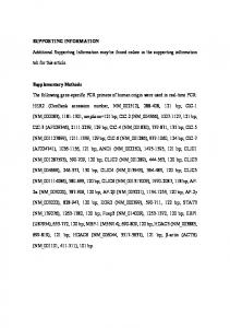
Figure S1: Diversity of the libraries – The different libraries are intended to harbor the same distribution of amino acids at the 4 varied positions. We measured these distributions by sequencing samples from the initial libraries. A. Sequence logos showing the entropies of the various amino acids at the four positions: the distribution is non-uniform but similar from one library to the next. B. More quantitatively, the distance between distributions is estimated using the Jensen-Shannon divergence: if qa` is the frequency of amino acid CDR3 `, the Jensen-Shannon divergence between libraries k and ` is defined as P of` library P ka in the k ` k ` /q ) + ln(q /q q ln(q q a a ). This divergence is found to be 5 to 10 times larger than expected from a a a a a a sampling noise. This represents the experimental precision at which we were able to introduce the same diversity in each library. These differences of frequencies between initial libraries are, however, much smaller than the differences of frequencies before and after a round of selection within a same library.

7

CA1 CA2 CA3 CA4 CA5 CA6 C1 CH1 CO1 F1 F2 F3 F4 F5 H1 H2 H3 L1 R1 S1 HG HL HM

CA1 CA2 CA3 CA4 CA5 CA6 C1 CH1 CO1 F1 F2 F3 F4 F5 H1 H2 H3 L1 R1 S1 HG HL HM

1.0 0.9 0.8 0.7 0.6 0.5 0.4 0.3 0.2 0.1 0.0

frequency round 3 (replica)

Figure S2: Sequence similarities between frameworks – Similarity between two frameworks is measured as the fraction of common amino acids in an alignment of their two sequences. Only the library-specific part of the frameworks (Figure 1) defined in Figure S17 is considered here. In most cases, the sequence similarity is in the range 30-60%.

frequency round 3 Figure S3: Reproducibility – To assay the reproducibility of the experiments, two independent selections of the mixture of 24 libraries were performed against the DNA target and the frequencies of the sequences were compared at the third round: the high correlation between the two results indicates high reproducibility.

8

A

Relative entropy

sites

S1 / PVP

F3 / PVP

sites

B

C sites

F3 / DNA

D sites

HG / DNA

E sites

CH1 / DNA

amino acids

Figure S4: Library and target specificities – Relative entropies of the different amino acids at the third round of different experiments; the relative entropy is calculated per site as fia ln(fia /qia ) where fia is the frequency of amino acid a at position i in the third round and qia in the initial library (round 0). A and B show that the consensus sequence is framework dependent. B and C show that it is target specific. Finally, C, D and E provide further evidence of framework dependency. (White squares indicate amino acids not represented in the population).

9

B

Pearson correlation : 0.9 frequencies Mix 24 amplified

A

frequencies Mix 24

frequencies

Figure S5: Biases in amplifications – Comparison of the composition of the mixture of 24 libraries before and after amplification in absence of selection. A. Differences of frequencies, showing that only the S1 and CH1 libraries are enriched. B. Correlations between the frequencies (same data).

round 1

round 2

frequencies

frequencies

Figure S6: Target-dependent hierarchy – Figure 2 shows that a mixture of 24 libraries selected against the DNA target is dominated by the HG framework while a mixture of 21 libraries that excludes the HG library is dominated by the CH1 framework. As shown in this figure, when the same mixture of 24 libraries is selected against the PVP target, a different framework, the S1 framework, dominates (consistently, it also dominates when screening the mixture of 21 libraries, which includes S1).

10

Figure S7: Variations in the values of extreme selectivities – When sampling N random variables from the extreme probability density fκ (x) given by Eq. (4), the value sr of the variable of rank r is distributed with a mean s¯r and standard deviation δsr . The ratio δsr /¯ sr is largest for the very top sequences, as shown here based on numerical simulations. This observation is consistent with deviations of the data from a power law observed for the very top selectivities even when κ > 0 and when the overall fit with an extreme value distribution is good (Figures 4A-B).

3

⌧ˆ

10

10

2

Data P (S  s)

Data s

B]

Model

P (S  s)

Estimated

Estimated  ˆ

A]

10

3

Threshold

10

3

Threshold s

Model s

Figure S8: EVT analysis for the selection of the HG library against the DNA target (data shown in Figure 3B). A fit of the general model gives κ = 0.26 ± 0.21, τ = 5.7 × 10−3 ± 1.5 × 10−3 while a fit of the exponential model (κ = 0) gives τ0 = 8 × 10−3 ± 1.4 × 10−3 ; the exponential model is excluded with a p-value 1.4 × 10−3 , in favor of κ > 0. Note that the threshold s∗ = 10−3 above which the fit is stable and good is much below the value of the selectivity above which a power law is observed in Figure 3B, of the order of s = 10−2 .

11

B]

10

3

Model P (S  s)

Data s

4

⌧ˆ

10 Estimated

Estimated  ˆ

Data P (S  s)

A]

10

3

Threshold

10

3

Threshold s

Model s

Figure S9: EVT analysis for the selection of the F3 library against the PVP target (data shown in Figure 3D). A fit of the general model gives κ = 0.07 ± 0.21, τ = 3.1 × 10−4 ± 8 × 10−5 while a fit of the exponential model (κ = 0) gives τ0 = 3.4 × 10−4 ± 6 × 10−5 ; the exponential model is excluded with a p-value 0.75, which is non significant. This data is therefore consistent with an exponential model κ = 0.

2

⌧ˆ

10

10

2 Data P (S  s)

Data s

B]

Model P (S  s)

Estimated

Estimated  ˆ

A]

10

3

Threshold

10

3

Threshold s

Model s

Figure S10: EVT analysis for the selection of the CH1 library against the DNA target (data shown in Figure 3C). A fit of the general model gives κ = −0.62 ± 0.25, τ = 2.5 × 10−2 ± 8 × 10−3 while a fit of the exponential model (κ = 0) gives τ0 = 1.5 × 10−2 ± 4 × 10−3 ; the exponential model is excluded with a p-value 10−2 , in favor of κ < 0.

12

2

⌧ˆ

10

10

2

Data P (S  s)

Data s

B]

Model P (S  s)

Estimated

Estimated  ˆ

A]

10

3

Threshold

10

3

Threshold s

Model s

Figure S11: EVT analysis for the selection of the F3 library against the DNA target (data not shown in the main text). A fit of the general model gives κ = 0.97 ± 0.38, τ = 2 × 10−3 ± 8 × 10−4 while a fit of the exponential model (κ = 0) gives τ0 = 7.5 × 10−3 ± 10−3 ; the exponential model is excluded with a p-value < 10−4 , in favor of κ > 0.

4

⌧ˆ

10

10

2

Data P (S  s)

Data s

B]

Model

P (S  s)

Estimated

Estimated  ˆ

A]

10

3

Threshold

10

3

Threshold s

Model s

Figure S12: EVT analysis for the selection of the N1 library in the mixture of 24 libraries against the PVP target (data not shown in the main text). A fit of the general model gives κ = 0.38 ± 0.21, τ = 1.3 × 10−4 ± 3 × 10−5 while a fit of the exponential model (κ = 0) gives τ0 = 2.2 × 10−4 ± 3 × 10−5 ; the exponential model is excluded with a p-value < 10−4 , in favor of κ > 0.

13

Figure S13: Scaling of the best binder with the library size – To estimate the gain that sampling m times more the same library may provide as a function of the shape parameter κ, we show here the expected difference E[s01 − s1 ] between the maximum s01 of mN samples drawn with probability density fκ (x) from Eq. (4) and the maximum s1 of N sub-samples. The plain lines are based on Eq. (S3) with τ = 1 and N = 105 and the dots are the results of numerical simulations (averaged over many draws), showing a good agreement between the two. Note how E[s01 − s1 ] depends more strongly on κ than on m.

Figure S14: Stability of the shape parameter κ for non-random sub-samples of a same library – To test whether non-random sub-libraries may be expected to be described by the same shape parameter as the library from which they originate, we consider here the results of the selection of library S1 against PVP (Figure 3A), for which the consensus CDR3 has amino acids sequence GWYT and we make four nonoverlapping sub-libraries consisting of sequences with CDR3 at distance d = 1 to 4 from this consensus, where the distance just counts the number of amino acid differences (number of mutations). This figure shows the selectivity versus the rank of the sequences in these sub-libraries. An EVT analysis indicates that κ(d = 1) = 0.33 ± 0.39, κ(d = 2) = 0.40 ± 0.26, κ(d = 3) = 0.30 ± 0.23, κ(d = 4) = 0.53 ± 0.22: all these values are comparable to the value κ = 0.44 ± 0.22 of the shape parameter for the full library. 14

A

Relative entropy

sites

S1 / amplification

B sites

HG / amplification

CH1 / amplification sites

C

Nurseshark in Mix21 again

A]

CO / amplification

Round 3

Sites

sites

D

amino acids

Nurseshark in Mix24 agains

Sites

Figure S15: Amplification bias – Relative entropy between frequencies of CDR3 sequences before and after amplification without selection, showing an enrichment in glutamine (represented by the letter Q). The Roundcodon, 3 results presented in the paper exclude sequences with an amber which is responsible for this effect (see supplementary experimental methods), but, in most experiments with selection, glutamine does not appear in the selected consensus sequence and considering the amber code as coding for an amino acid or for a stop codon has no incidence on the conclusions.

B]

Relative entropy

S1 in Mix 21 / PVP sites

round 3

amino acids S1 in Mix 24 / PVP

Relative entropy

sites

round 3

amino acids

B

Selectivity Nurseshark in Mix24 selectivity S1in Mix24 / PVPPVP

A

Amino acids

selectivity S1in Mix21 / PVP Selectivity Nurseshark in Mix21 PVP

Figure S16: Reproducibility of selections against the PVP target – The results of two experiments of selection against the PVP target, one starting from a mixture of 24 libraries and the other from a subset of 21 libraries, which each are dominated by the S1 library, not only lead to an identical consensus sequence (panel A) but to reproducible results by EVT analysis (Table S3). In this case, not only are the initial populations different, but also potentially the targets since the experiments were performed 1.5 year apart and PVP is subject to aging: this may explain the imperfect correlations between frequencies (panel B; by contrast, the selection of the F3 library against PVP was performed at the same time than the selection of the mixture of 24 libraries and differences in consensus sequences cannot be due to differences of the targets in this case).

15

CA1|CatFish CA2|CatFish CA3|CatFish CA4|CatFish CA5|CatFish CA6|CatFish C1|Cattle CH1|Chicken CO1|Coelacanth F1|Frog F2|Frog F3|Frog F4|Frog F5|Frog H1|Human H2|Human H3|Human L1|LittleSkate R1|Rabbit S1|NurseShark HG|Human(germline) HL|Human(matured) HM|Human(bnAb)

PAMAATELIQPDSVVIKPGETLTITCRVSGASITDSSSHYGTAWIRQPAGKGLEWFN--PAMAAVELTQVTSVMLKPGDSLTLSCKVSGYSVTDNS--YATAWIRQPAGKGLEWIN--PAMAGEELTQPASMTVQPSQSLSINCKVS-YSVTS----YYTAWIRQPAGKGLEWIG--PAMAEIRLDQSSAVVKRPGESVKISCKINGLDMTA----HYMHWIRQKPGKGLEWVG--PAMASQTLIESDSVIIKPDQSHKLTCTASGFNFGG--SWMA--WIRQSPGKGLEWVA--PAMAGQSLTSLGSVVKRPGESVTLSCTLSGFSLDS----YWMSWIRQKPGKGLEWIG--PAMAQVQLRESGPSLVKPSQTLSLTCTTSGFSLTSYGVTW----FRQAPGKGLEWLG--PAMAAVTLDESGGGLQTPGGTLSLVCKGSGFTFND--YAMG--WMRQAPGKGLEWVA--PAMADVTLTESGGDVKRPGESLKLSCKASGFDFSS--YWMG--WVRQPPGKGLEFVS--PAMAEVTVSLSVPELVKPSEKLKLVCKVSGALITDGSKIHAVNYIRQFSGSGLEFLA--PAMAQITLDQPGSAAVKPSETVKLSCKVS---VSVTSYAWA--WIWQAPGKGLEYIG--PAMAQISLMESGPGTVKPTTTLQLTCKVTGASLTDSTNMYGVLWVRQPAGKGLEWLG--PAMASQTLQESGPGTVKPSESLRLTCTVSGFELTS----NAVTWIRQPPGKGLEWIG--PAMADVQLDQSESVVIKLGGSHKLSCTASGFTFSD--YWMS--WIRQAPGKGLERVF--PAMAQVTLRESGPALVKPTQTLTLTCTFSGFSLSTSGMCVS--WIRQPPGKGLEWLA--PAMAQVQLQQSGPGLVKPSQTLSLTCAISGDSVSSNSAAWN--WIRQSPSRGLEWLG--PAMAEVQLVQSGAEVKKPGESLRISCKGSGYSFTS----YWISWVRQMPGKGLEWMG--PAMADIVLTQPKTEAATPGGSITLTCKVSGFALSS--YAMH--LVRQAPGQGLEWLL--PAMAQS-LEESRGGLIKPGGTLTLTCTASGFTISS--YYMC--WVRQAPGKGLEWIG--PAMAEVTLIQPEAENGHPGGSMRLTCKTSGFDLDS--YAMS--WVRQVPGQGLEWIV--PAMAQLQLQESGPGLVKPSETLSLTCTVSGGSISSSSYYWG--WIRQPPGKGLEWIG--PAMAQLQLQESGPGLVKPSETLSLTCIVSGGSIGTTDHYWG--WIRQSPGKGLEWIG--PAMAQPQLQESGPTLVEASETLSLTCAVSGDSTAACNSFWG--WVRQPPGKGLEWVGSLS

CA1|CatFish CA2|CatFish CA3|CatFish CA4|CatFish CA5|CatFish CA6|CatFish C1|Cattle CH1|Chicken CO1|Coelacanth F1|Frog F2|Frog F3|Frog F4|Frog F5|Frog H1|Human H2|Human H3|Human L1|LittleSkate R1|Rabbit S1|NurseShark HG|Human(germline) HL|Human(matured) HM|Human(bnAb)

--SIYYDGG-INKKDSLKDKFVISRDTSSSTVILTGQDMQTEDTAVYYCAR --YIWGGGS-SYHKDSLKSKFSISKDGSSSTVTLRGQNLQTEDTAVYYCAR --YISNNGG-TVYSDKLKNKFSISRDTATNTITIRGQNLQTEDTAVYYCAR --RMDAGKNQAIYAESLKNQFTLTEDVPASTQCLEVKSLRTEDTAVYYCAR --TISDTSGSKYYSSALKGRFTISRDNSKMEVYLHMASVRTEDTAVYYCAR --RIDSGTG-TTFTQSLKGQFSITKDTNKNMLYLEVKSLKTEDMAVYYCAR ---EINNNGFMDRNPDLKSRLNITREISLSQVSLSLSRVTPEDTAVYYCAR --GIRNDGSYPIYGAALKGRATISRDNGQSTVRLQLNNLRAEDTGTYYCAR --ILEYDSDRRYFGQSLKGRFTTSRENSNSMLYLQMNSLRVEDTAMYYCAR ---HINYAAGTALNPDLKSRLTLSRDTAKNEAYLEISGMTAGDTAMYYCAR ---YLGSDGSSNPASSLKSRVTFTRDTSKNEIYLQMTSMKSEDSGTYYCAR ---GIYYNGNTDYATTLKGRLTLSRDTNKGEVYFKLTEAKTEESATYYCAR ---VIASNGGTAFADSLKNRVTITRDTGKKQVYLQMNGMEVKDTAMYYCAR --YIRHDGGTTNYADSLKGRFTISRDSKNNKLYLQMNNLHTEDTAVYYCAR ---RIDWDDDKYYSTSLKTRLTISKDTSKNQVVLTMTNMDPVDTATYYCAR -RTYYRSKWYNDYAVSLKSRITINPDTSKNQFSLQLNSVTPEDTAVYYCAR --RIDPSDSYTNYSLSLKGHVTISADKSISTAYLQWSSLKASDTAMYYCAR ---RYFSSSNKQFAPGLKSRFTPSTDHSTNIFTVIARNLKIEDTAVYYCAR --AIG-SSGSAYYASWLKSRSTITRNTNENTVTLKMTSLTAADTATYFCAR ---YSYGSYSNDYAPALKDRFTASIDTSNNIFALEMKSLKIEDTAIYYCAR --SIYYS-GSTYYNPSLKSRVTISVDTSKNQFSLKLSSVTAADTAVYYCAR --TTYYS-GKTYYNPSLKSRVTISIDTSKNHFSLRLISVTAADTAVYHCAR HCASYWNRGWTYHNPSLKSRLTLALDTPKNLVFLKLNSVTAADTATYYCAR

Figure S17: Amino acid sequences of the frameworks – Multiple sequence alignment of the library-specific part of the frameworks (Figure 1). The organism from which the sequence originate is indicated. See Dataset S1 for the nucleotide sequences.

16

A

Exponential

B

C

Normal

Cauchy

Figure S18: Illustration of the EVT analysis with simulations from standard distributions – We numerically drew 105 samples from the exponential, normal and Cauchy distributions and analyzed in each case the top 103 values by the same procedure that we used to analyze our data in Figure 4. A. For the exponential distribution, a fit of the general model gives κ = −0.02 ± 0.05, τ = 1.04 ± 0.08 while a fit of the exponential model (κ = 0) gives τ0 = 1.02 ± 0.06; the exponential model is excluded with a p-value 0.81, which is non significant. These results are consistent with the analytical result κ = 0. B. For the normal distribution, a fit of the general model gives κ = −0.07 ± 0.06, τ = 0.34 ± 0.03 while a fit of the exponential model (κ = 0) gives τ0 = 0.31 ± 0.2; the exponential model is excluded with a p-value 0.14, which is non significant. These results are consistent with the analytical result κ = 0. The exponential and normal distributions are examples of two different distributions that belong to the same class of extreme value statistics. C. For the Cauchy distribution, a fit of the general model gives κ = 1.03 ± 0.12, τ = 30.3 ± 3.8 and the exponential model is excluded with a p-value < 10−4 , which is significant. These results are consistent with the analytical result κ = 1.

10

-1

10

-2

10

-3

10

0

10

1

10

2

Figure S19: Fit of the generalized Pareto distribution versus a power law distribution – The data shown in red is the same as in Figure 3B (HG library against DNA target). The green dotted line indicates the best fit to a generalized Pareto distribution, using the values of κ and τ inferred in Figure S8. This graph shows that the fit extends far beyond the range of selectivities that may be fitted by a power law (black dotted line).

17

5

Supplementary code

The following code is in the format of an IPython notebook. It assumes that the data has been processed and formatted into a file (here named Data/S1_PVP.dat and containing the results of the selection of the S1 library against the PVP target as in Figures 3A and 4) with 3 columns separated by tabs containing respectively, a sequence or a label of the sequence, an estimation of the selectivity of this sequence, and an estimation of the error in the value of the selectivity. One parameter, s_star, must be set by hand in cell [6] based on the plots obtained in cell [5]. In [1]: %matplotlib inline import matplotlib.pyplot as plt import numpy as np import scipy import scipy.stats as ss

In [2]: # Path to the input file: data_file = ’Data/S1_PVP.dat’ # Reading the data into dictionaries for selectivities and errors: sel_dict, err_dict = dict(), dict() for line in open(data_file , ’r’): seq, sel, err = line.split(’\t’) sel_dict[seq] = float(sel) err_dict[seq] = float(err)

5.1

Selectivity versus rank

In [3]: # Sorting the data by decreasing values of selectivies: seq_sorted = sorted(sel_dict, key=lambda s: -sel_dict[s]) sel_sorted = [sel_dict[s] for s in seq_sorted] err_sorted = [err_dict[s] for s in seq_sorted] # Figure 3A: plt.rcParams[’figure.figsize’] = 5, 5; plt.rc(’font’, size=16) plt.loglog(range(len(sel_sorted)), sel_sorted,’or’, lw = 2); plt.xlabel(’rank’, fontsize=20); plt.ylabel(’selectivity’, fontsize=20) plt.axis([0, 1.3*len(sel_sorted), sel_sorted[-1], 1.3*sel_sorted[0]]); plt.grid(’on’)

18

In [4]: def log_likelihood_fct_exp(para, data_sorted): ’’’ Log-likelihood function for the exponential model ’’’ tau, mu = para[0], min(data_sorted) return -sum([np.log(np.exp(-(x-mu)/tau)/tau) for x in data_sorted[:-1]]) def log_likelihood_fct_evt(para, data_sorted): ’’’ Log-likelihood function for the general model ’’’ kappa, tau, mu = float(para[0]), para[1], min(data_sorted) return -sum([np.log((1+(x-mu)*(kappa/tau))**(-((kappa+1))/kappa)/tau)\ for x in data_sorted[:-1]]) def info_mat_exp(tau, data_sorted): ’’’ Observed information matrix for the exponential model ’’’ mu = min(data_sorted) data = [x-mu for x in data_sorted[:-1]] return -1/sum([(tau-2*x)/tau**3 for x in data]) def info_mat_evt(para, data_sorted): ’’’ Observed information matrix for the general model ’’’ matrix = np.zeros((2,2)) kappa, tau, mu = para[0], para[1], min(data_sorted) data = [x-mu for x in data_sorted[:-1]] matrix[0][0] = -sum([(-kappa*x**2+tau**2-2*tau*x)/(tau*(kappa*x+tau))**2 for x in data]) matrix[0][1] = -sum([x*(tau-x)/(tau*(kappa*x+tau)**2) for x in data]) matrix[1][0] = -sum([x*(tau-x)/(tau*(kappa*x+tau)**2) for x in data]) matrix[1][1] = -sum([(kappa*x*(kappa*(kappa+3)*x +2*tau)\ -2*(kappa*x+tau)**2*np.log(1+kappa*x/tau))/(kappa**3*(kappa*x+tau)**2) for x in data]) return np.linalg.inv(matrix) def threshold_scan(sel_sorted, min_points, para=[1,0.001]): ’’’ Maximum likelihood estimation of kappa, tau for different values of the threshold. min_points sets the minimum number of points to be kept ’’’ para_list, err_list = list(), list() for i in range(len(sel_sorted), min_points, -1): para = scipy.optimize.fmin(log_likelihood_fct_evt, para,\ args=(sel_sorted[:i],), disp=False, maxiter=1000) para_list.append(para) err = info_mat_evt(para, sel_sorted[:i]) err_list.append([1.96*np.sqrt(err[1][1]), 1.96*np.sqrt(err[0][0])]) return para_list, err_list In [5]: min_points = 50 para_list, err_list = threshold_scan(sel_sorted, min_points) # Figure 4A: plt.rcParams[’figure.figsize’] = 12, 5; plt.rc(’font’, size=12) plt.subplot(121) plt.errorbar(sel_sorted[min_points:][::-1],[p[0] for p in para_list],\ [e[0] for e in err_list],fmt=’k.’,linewidth=3) plt.plot(sel_sorted[min_points:][::-1],[p[0] for p in para_list],’go’,markersize=8) plt.xlabel(r’threshold $s^*$’,fontsize=20); plt.ylabel(r’estimated $\kappa$’,fontsize=20) plt.subplot(122) 19

plt.errorbar(sel_sorted[min_points:][::-1],[p[1] for p in para_list],\ [e[1] for e in err_list],fmt=’k.’,linewidth=3) plt.plot(sel_sorted[min_points:][::-1],[p[1] for p in para_list],’go’,markersize=8) plt.xlabel(r’threshold $s^*$’,fontsize=20); plt.ylabel(r’estimated $\tau$’,fontsize=20) plt.tight_layout();

In [6]: # Choice of the treshold based on previous plots: s_star = .0004

5.2

Parameters of the best fit

In [7]: # Truncation of the data given s_star: sel_trunc = [s for s in sel_sorted if s > s_star] mu = min(sel_trunc) N_samples = len(sel_trunc) # Maximum likelihood estimation of tau under the exponential model: print ’Exponential fit:’ para = scipy.optimize.fmin(log_likelihood_fct_exp,[.01],args=(sel_trunc,), maxiter=10000) tauexp = para[0] print ’tau_exp = %.5f\n’ % tauexp # Maximum likelihood estimation of kappa, tau under the general model: print ’General fit:’ para = scipy.optimize.fmin(log_likelihood_fct_evt, [.5,.01], args=(sel_trunc,), maxiter=10000) kappa, tau = para[0], para[1] print ’kappa = %.3f, tau = %.5f’ % (kappa, tau) Exponential fit: Optimization terminated successfully. Current function value: -1249.910350 Iterations: 21 Function evaluations: 42 tau_exp = 0.00028 General fit: Optimization terminated successfully. 20

Current function value: -1267.475534 Iterations: 49 Function evaluations: 95 kappa = 0.453, tau = 0.00016

5.3

Diagnosis plots for the fit

In [8]: # Q-Q plot and P-P plots with the general model: x_range = np.linspace(0, 1-1./N_samples, num=N_samples) sel_model = [((1-x)**(-kappa)-1)/kappa for x in x_range] sel_pp = [1-(1+kappa*(s-mu)/tau)**(-1/kappa) for s in sel_trunc[::-1]] # Figure 4B: plt.rc(’font’, size=14) plt.subplot(121); plt.title(’Q-Q plot (general model)’, fontsize=18); # Q-Q plot plt.plot([0,max(sel_model)],[mu,mu+tau*max(sel_model)],’k-.’,linewidth=2); plt.errorbar(sel_model, sel_trunc[::-1], yerr=err_sorted[:N_samples][::-1],\ fmt=’b.’, markersize=15) plt.xlabel(’model’, fontsize=20); plt.ylabel(’data’, fontsize=20) plt.subplot(122); plt.title(’P-P plot (general model)’, fontsize=18); # P-P plot plt.plot([0,1],[0,1],’k--’, lw=2) plt.plot(sel_pp, x_range ,’r’,lw=3) plt.xlabel(’model’, fontsize=20); plt.ylabel(’data’, fontsize=20);

In [9]: # Q-Q plot and P-P plots with the exponential model: plt.subplot(121); plt.title(’Q-Q plot (exponential model)’, fontsize=18); # Q-Q plot sel_model = [-np.log(1-x) for x in x_range] plt.plot([0,max(sel_model)],[mu,mu+tau*max(sel_model)],’k-.’,linewidth=2); plt.errorbar(sel_model, sel_trunc[::-1], yerr=err_sorted[:N_samples][::-1],\ fmt=’b.’, markersize=15); plt.xlabel(’model’, fontsize=20); plt.ylabel(’data’, fontsize=20); plt.subplot(122); plt.title(’P-P plot (exponential model)’, fontsize=18); # P-P plot sel_pp = [1-np.exp(-(s-mu)/tauexp) for s in sel_trunc[::-1]] plt.plot([0,1],[0,1],’k--’, lw=2)

21

plt.plot(sel_pp, x_range ,’r’,lw=3); plt.xlabel(’model’, fontsize=20); plt.ylabel(’data’, fontsize=20);

5.4

Significance of κ 6= 0

In [10]: def distr_LikeRatioTest(tauexp, N_samples, N_draws): ’’’ Making a null distribution for a likelihood ratio test of kappa not 0’’’ distr = list() for n in range(N_draws): # Drawing samples from the exponential model: sel_rand = np.random.exponential(tauexp, N_samples) # Fitting them by maximum likelihood estimation with the general model: para = scipy.optimize.fmin(log_likelihood_fct_evt, [.5,.01],\ args=(sel_rand,), disp=False, maxiter=1000) distr.append(2*(log_likelihood_fct_exp([tauexp], sel_rand)\ - log_likelihood_fct_evt(para, sel_rand))) return distr In [11]: # null distribution: N_draws = 10000 distr = distr_LikeRatioTest(tauexp, N_samples) # experimental value: dL_sel = 2*(log_likelihood_fct_exp([tauexp], sel_trunc)\ - log_likelihood_fct_evt([kappa,tau], sel_trunc)) # p-value: p_val = sum([1 for dL in distr if dL > dL_sel])/(1.*len(distr)) if p_val > 0: print ’p-value against the exponential model: %.e’ % p_val else: print ’p-value against the exponential model: < %.e’ % 1./N_draws p-value against the exponential model < 1e-04 In [12]: # Representation of the estimated kappa from experimental measurements # versus the distribution of estimated kappa for samples from an exponential model: 22

plt.hist(distr, 100, label=r’$\kappa = 0$’) plt.axvline(dL_sel, color=’r’, lw=3, label=’data’); plt.legend(bbox_to_anchor=(1.2,1.03)); plt.xlabel(’test statistics’, fontsize=20); plt.ylabel(’counts’, fontsize=20);

23