Aldrich, St. Louis, MO), covered with foil, and grown at 37°C with 275-rpm shaking. ..... P., Groves, J. T., and Ajo-Franklin, C. M. (2010) Engineering of a synthetic ...
Plots of frontier orbitals and spin-dependent transmission coefficients. The spin dependent transport calculations show similar behaviour for T(E) for both up spin ...
prepared by placing a drop of the dilute chloroform solution of nanoparticles on the carbon coated copper grids and allowing the solvent to evaporate at room ...
Sci. Rep. 1996, 25, 1-140. (S15) Montgomery, D. C., Runger, G. C.; Applied statistics and probability for engineers 6th. Edition, Wiley, 2014, p. 447-448. S12.
for promoting a stabilization of the cubic structure, whereas for Ta-N, metallic .... The defect-free structures show a transition region between x = 0.62 (LDA) and ...
Temperature ramp tests of B-linker and Y-scaffold were carried out on a Cary100 UVâVis spectrometer (Agilent Technologies) equipped with a temperature.
Nov 21, 2012 - Aromatic peptides, self-assembly, peptide nanotubes, mechanical properties ... structures formed by mixing two aromatic peptides known.
Aug 25, 2016 - Tuning the Mechanical Properties of Polymer ...... ACS Macro Lett. ... Palli, B.; Padmanabhan, V. Chain flexibility for tuning effective interactions ...
Ni distance in pentamer (8.41 Ã ). The Ni-S bond from PBED (2.14 Ã ) and HSE06 (2.14 Ã ) are close to the experimental values (2.15 Ã ).8 The other bond lengths ...
Tuning Coupling Behavior of Stacked Heterostructures Based on MoS2, WS2, and WSe2. Fang Wang, Junyong Wang, Shuang Guo, Jinzhong Zhang, Zhigao ...
herring sprat c). Diatom bloom. Summer. c o m m u n itie s. S1 Fig. Seasonal development of (a) phytoplankton biomass, (b) zooplankton biomass,.
For negligible âk, a similar expression can be found for the frequency shift in dependence on the mass change âm. In this case a Taylor series expansion is ...
Sean T. Hemp, Amanda G. Hudson, Michael H. Allen, Jr., Sandeep S. Pole, Robert B. Moore, and Timothy E. Long*. Macromolecules and Interfaces Institute, ...
The effect of the coverslip (second anchoring surface) was more apparent for biphasic ... dispersions being squeezed out by the weight of the coverslip.
a) First aerial photographic series: 1927-2007 (15 records), PHTH-WL; ... series: 1927-2008 (23 records), WDL-RM; d) Complete series (without 1927 and 1929.
In order to compute the induced dipole moment on the CNT due to the inside (out) water molecules, a QM/MM setup was used, similar to the one previously.
analyses, hemolysates were prepared by dilution of blood cells at 1:10 in water. .... 760.5 (824.8). 793 (783.9). 728 (865.8) d (0.08). 0.675. Global assessment of.
The antibodies used are listed as follows: anti-Nrf2 (Abcam, ab62352, 1: 1000), anti-AMPK (CST, 2532, 1: 1000), anti-p-AMPK (CST, 2535, 1: 1000), anti-PERK ...
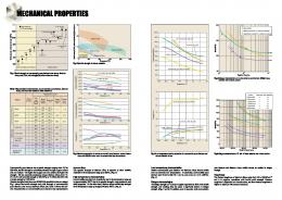
other properties. On the other hand, titanium alloys exhibit high strength ..... Table 5:Difficulties in cutting and shearing titanium and countermeasures. Difficulties.
The mechanical properties of materials are important to engineers allowing the selection of the proper material and desi
Tuning Mechanical Properties of Nanocomposites with Bimodal Polymer Bound Layers
Erkan Senses and Pinar Akcora Department of Chemical Engineering and Materials Science Stevens Institute of Technology, Hoboken, NJ 07030 USA
Figure S1. TEM images of 13 nm Silica nanoparticles in PMMA (left image) and PS (right image). Composite films are cast from THF. PMMA matrix consists of 50:50 blends of short (4.3 kg/mol) and long (96 kg/mol) chains. PS matrix consists of 50:50 blends of short (5 kg/mol) and long (100 kg/mol) chains. Particle loadings are 15 wt% in both samples.
Figure S1 shows the effect of solvent on bound layer and dispersion. The choice of solvent influences interaction between polymer and nanoparticles and consequently controls nanoparticle dispersion in polymer nanocomposites. Figure S1 (left image) shows micron-size aggregates of 13-nm Silica particles in PMMA, cast from THF, which is a good solvent for PMMA. THF displaces chains on particle surfaces, preventing formation of a physically bound polymer layer. The observed aggregation reveals the effect of bound layers on particle dispersion. When we changed the polymer to polystyrene, we obtained similar phase separated particles (Figure S1, right image).
Figure S2. TEM images for (a) 13 nm and (b) 55 nm SiO2 nanoparticles in 96/4.3 blend PMMA matrix (50/50 vol%). Particle loading is 15 wt% in both samples.
Number % [a.u.]
Bare silica
100 Weight [%]
Bare silica L=0.0 L=0.3 L=0.7 L=0.95 L=1.0
10
100 Size [nm]
96
92 88
84
80
1000
L
200 400 600 Temperature [°C]
Figure S3. (Left) Hydrodynamic size distributions of 55 nm SiO2 nanoparticles adsorbed with 68-2.6 kg/mol PMMA blends at varying ϕL. (Right) Weight loss curves of corresponding particles are measured in TGA.
30 kg/mol PMMA 2.6 kg/mol PMMA CH3
O
Absorbance (a.u.)
O
S
C=O
CH2
C
n
Cl
C O CH3
O CH3
C=C 4000
3000
2000
1000
0
Wavenumber (cm-1)
Figure S4. FTIR spectra of PMMA homopolymers at 30 and 2.6 kg/mol.
a
c
d
b
Figure S5. TEM images of 55 nm particles adsorbing 68/2.6 kg/mol PMMA blends at varying blend compositions: (a) 50/50 vol%, (b) 100/0 vol%, (c) 70/30 vol%, (d) 30/70 vol% dispersed in 28 kg/mol PMMA matrix. Images next to (c) and (d) are at low magnification. Particle loading is 30 wt% in all composites. Zero-shear viscosities We obtained the zero shear viscosities η0 by fitting complex viscosity data to three-parameter Cross model
* 0 1 . We first obtained parameters for particle-free matrix as 0 1 Km
0,free 5162 Pa.s ,
K free 0.017 and m free 0.72 .
Then,
viscosity
parameters
for
the
nanocomposite samples were obtained by superposing the contributions of free and interphase. We kept the matrix contribution the same as the particle loading is constant, and only allow the interphase parameters to change in the composite viscosity to give * *free *int erphase . Because polymer is the same in the interphase, we kept the exponent the same for free chains
m free mint erphase 0.72 . We then obtained the parameters K int erphase and 0,interphase for each bound layer composition L. Contributions from free and interphase polymer and their superposition is illustrated on the composite with L = 1 in Figure S6. Fittings for all composites are shown in Figure S7. Fitting parameters for the interphase contributions in each sample are given in Table S1. The overall zero shear viscosity then becomes 0 0,free 0,int erphase .
*(Pa.s)
104
103 Exp. data L=1.0) Combined Matrix Interphase
2
10
101
0.1
1
10
100
1000
(rad/s) Figure S6. Complex viscosity response of composite with L = 1 obtained from linear viscoelastic results shown in Figure 4 and corresponding model fit. Solid lines are free and interphase polymer contributions to the composite viscosity.
h [nm] Fi gure S8. Relative zero-shear viscosities as a function of hydrodynamic size (h) of particles. Flat line is the Guth prediction for spherical particles at high loadings. Particle loading is 30 wt%.
Figure S9. Linear elastic modulus and loss tangent of nanocomposites with 12/2.6 kg/mol PMMA blend adsorbed on SiO2 (55 nm) nanoparticles dispersed in 28 kg/mol PMMA (T = 210 oC).
Inset shows reinforcement factor calculated from zero shear viscosity. Particle loading is 30
wt%.
Tg, Tf [oC]
135
Tf Tg
130 125 120 115
0 20 40 60 80 100
L
Figure S10. Glass transition (Tg) and fictive (Tf) temperatures of nanocomposites with varying long chain fraction in bound layer.