Supporting Text S1 Calcium signals driven by single channel ... - PLOS

Supporting Text S1 Calcium signals driven by single channel noise Alexander Skupin, Helmut Kettenmann and Martin Falcke

Contents 1

IP3 R model (Supporting Figure 1 and Table 1)

2 Derivation of the linearized system (Supporting Figure 2 and Table 2) 3 Deriving the solution (Supporting Figure 3)

3 6 10

3.1

Ca2+ dynamics . . . . . . . . . . . . . . . . . . . . . . . . . . . . . . . . . . 14

3.2

Boundary conditions . . . . . . . . . . . . . . . . . . . . . . . . . . . . . . . 17

3.3

Average concentrations . . . . . . . . . . . . . . . . . . . . . . . . . . . . . . 18

4 Green’s cell algorithm implementation

20

4.1

Gillespie algorithm . . . . . . . . . . . . . . . . . . . . . . . . . . . . . . . . 20

4.2

Parallel algorithm structure (Supporting Figure 4) . . . . . . . . . . . . . . 21

5 Spiking in dependence on IP3 and Ca2+ (Supporting Figure 5)

25

6 Population slopes (Supporting Figure 6)

27

1

Supporting Text S1 Skupin et al.

2

List of Figures 1

The DeYoung-Keizer model . . . . . . . . . . . . . . . . . . . . . . . . . . .

3

2

Linearization of the SERCA pump term . . . . . . . . . . . . . . . . . . . .

7

3

Sketch of the angles of two points in spherical coordinates . . . . . . . . . . 14

4

Scheme of the parallel Green’s cell model algorithm . . . . . . . . . . . . . . 22

5

Channel dynamics in dependence on IP3 and Ca2+ . . . . . . . . . . . . . . 26

6

Determination of population slope . . . . . . . . . . . . . . . . . . . . . . . 28

List of Tables 1

Transition rates for the DeYoung-Keizer channel model . . . . . . . . . . .

4

2

Dimensionless parameter definition . . . . . . . . . . . . . . . . . . . . . . .

8

Supporting Text S1 Skupin et al.

1

3

IP3 R model (Supporting Figure 1 and Table 1)

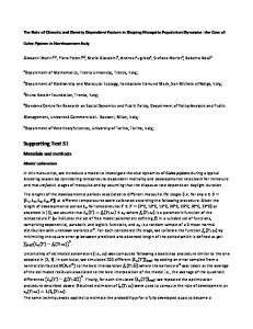
We use a modified version of the DeYoung-Keizer model (DKM), but the following derived reaction diffusion system and its solution can also be used with other channel models. The DKM assumes each IP3 R to consist of four identical subunits with 3 binding sites each. One binding site for IP3 , one for Ca2+ activating the subunit and another one for Ca2+ , which inhibits the subunit. The two binding sites for Ca2+ with a higher affinity for the activating site and a lower affinity for the dominant inhibiting site is a minimal choice to generate nonlinearities which are essential for Ca2+ induced Ca2+ release. Since each of the 3 binding sites can be free or occupied, a single subunit has 23 different states Xijk and 12 possible transitions, which can be visualized on a cube as shown in Supporting Figure 1A. a2C

A

X110

a5C

a5C

b1

b5 a2C

X111

b2

b3 b5

X100

1

X101

Po 0.5

b2 b1

a1I

b3

a3I

a4C X010

a5C a1I

a3I

b5 a4C

X000

X001

B

X011

b4 a5C

0 4 [IP3] (µM) 2

b5

0 0.01

1 [Ca ] (µM)

100

2+

b4

Supporting Figure 1: A: Scheme of the DeYoung-Keizer model for a single subunit. A subunit is active, if IP3 (I) is bound and Ca2+ (C) is only bound to the activating site, i.e. in state X110 . A channel opens if at least 3 of its 4 subunits are active. See text for more details and Supporting Table 1 for values of rates bi and rate constants ai . B: Stationary open probability Po defined by Equation (2) for the rate constants ai and rates bi given in Supporting Table 1.

The first index of Xijk specifies IP3 binding and is 1 if IP3 is bound and 0 otherwise. Analogously, the second index indicates Ca2+ binding to the activating site, and the last one corresponds to Ca2+ binding to the dominant inhibiting site. A subunit is active in the

Supporting Text S1 Skupin et al. a1 b1 a2 b2 a3 b3 a4 b4 a5 b5

20 (µMs)−1 20 s−1 0.001 (µMs)−1 0.03 s−1 2.6 (µMs)−1 20 s−1 0.025 (µMs)−1 0.1 s−1 10 (µMs)−1 1.225 s−1

4

IP3 binding with no inhibiting Ca2+ bound IP3 dissociation with no inhibiting Ca2+ bound Ca2+ binding to inhibiting site with IP3 bound Ca2+ dissociation from inhib. site with IP3 bound IP3 binding with inhibiting Ca2+ bound IP3 dissociation with inhibiting Ca2+ bound Ca2+ binding to inhib. site with no IP3 bound Ca2+ dissociation from inhib. site without IP3 Ca2+ binding to activating site Ca2+ dissociation from activating site

Supporting Table 1: Rates of the DKM used within simulations.

state X110 only and a channel will open if at least three of the four subunits are activated. The transitions between the states Xijk occur by stochastic binding and dissociation of signalling molecules to the corresponding binding sites. The rates for binding depend on the particular rate constants ai and on the Ca2+ concentration C and the IP3 concentration I, respectively, as shown in Supporting Figure 1A, whereas dissociation occurs with constant rates bi . Values are given in Supporting Table 1. The binding and unbinding of Ca2+ and IP3 in an ensemble of receptors lead to a fraction of channels pijk in the state Xijk . In the case of a large and homogeneous ensemble, the dynamics of pijk can be described by rate equations taking the dependence on the Ca2+ and IP3 concentration into account. In general these concentrations are not constant in time, and especially the Ca2+ concentration changes enormously by transitions from closed to open states and vice versa. We can determine the stationary values p¯ijk for constant Ca2+ and IP3 concentrations denoted by Cst and I, respectively. They are given by

p¯000 = γ1 d1 d2 d5

p¯100 = γ1 d2 d5 I ,

(1a)

p¯010 = γ1 d1 d2 Cst

p¯001 = γ1 d3 d5 Cst ,

(1b)

2 p¯011 = γ1 d3 Cst

p¯101 = γ1 d5 I Cst ,

(1c)

2 p¯111 = γ1 I Cst ,

(1d)

p¯110 = γ1 d2 I Cst

Supporting Text S1 Skupin et al.

5

where γ1−1 = (Cst + d5) (d1 d2 + Cst d3 + Cst I + d2 I) and di =bi /ai . With these relations we can determine the stationary open probability Po in dependence on Ca2+ and IP3 . Since a channel opens if three or four subunits are in the state X110 , the open probability takes the form Po = 4p3110 − 3p4110 ,

(2)

which is shown in Supporting Figure 1B in dependence on Ca2+ and IP3 for the rates given in Supporting Table 1. We observe a bell shaped dependence on Ca2+ and the monotonic increase of Po with increasing IP3 . The values of Po are in the range found experimentally [1, 2].

Supporting Text S1 Skupin et al.

2

6

Derivation of the linearized system (Supporting Figure 2 and Table 2)

To reflect the most important cytosolic properties, we take free [Ca2+ ] one mobile [B] and one immobile buffer [Bi ] in the cytosol into account leading to the following reaction diffusion system N

cl X ∂[Ca2+ ] = DCa ∇2 [Ca2+ ] − Pp [Ca2+ ] + Pl ([E] − [Ca2+ ]) + Jj (t) δ (r − ri ) ∂t

(3a)

j=1

− k + [B][Ca2+ ] + k − ([B]T − [B]) − ki+ [Bi ][Ca2+ ] + ki− ([Bi ]T − [Bi ]) ∂[B] = DB ∇2 [B] − k + [B][Ca2+ ] + k − ([B]T − [B]) ∂t ∂[Bi ] = −ki+ [Bi ][Ca2+ ] + ki− ([Bi ]T − [Bi ]), ∂t

(3b) (3c)

where we applied the buffer conservation and used a linear pump and leak flux with the flux constants Pp and Pl . Jj (t) is the stochastically in time varying channel cluster current of the jth cluster, k + and k − denote the capture and dissociation rates of the buffers, and [B]T and [Bi ]T are the total mobile and immobile buffer concentrations. The linearization 2+ 2

] 2+ ] is lin nl = V max [Ca[Ca of the nonlinear pump term Jpump 2+ ]2 +K 2 of the Form Jpump = Pp [Ca D

shown in Supporting Figure 2, where KD is the dissociation constant of the pump. The √ lin nl parameter Pp = 3V max /(4KD ) is determined by Jpump = Jpump at the inflection point nl of Jpump . The linearization matches the nonlinear pump term rather well for the most

relevant range up to 2 KD . We introduce dimensionless concentrations by

c=

[Ca2+ ] [B] [Bi ] [E] , b= , bi = , e= KB [B]T [Bi ]T KB

(4)

where KB denotes the dissociation constant of the mobile buffer. For one channel cluster,

Supporting Text S1 Skupin et al.

7

Jpump / Vmax

3 non-linear linear

2

1

0 0

1

2 3 2+ c = [Ca ] / KD

4

5

Supporting Figure 2: Linearization of the SERCA pump term. The linearization (red) of
2 −1 (black) around its inflection nl = V max [Ca2+ ]2 [Ca2+ ]2 + KD the nonlinear term Jpump point leads to a quantitatively well approximation over a large concentration range. For regions, where the concentration is even higher than 2 KD , i.e. close to open channels, the dynamics is mostly determined by the diffusion and channel terms.

this leads to Pp ∂c Pl DCa ∇2 c − bc + (1 − b) + + (¯ e − c) − + c = 2 + ∂t L k [B]T k [B]T k [B]T   [Bi ]T ki− KB J(t) + 1 − bi − bi c + 3 − δ(r − r 0 ) − [B]T k KBi L k [B]T 1 ∂b DB = 2 − ∇2 b − bc + (1 − b) T k − ∂t L k   [Bi ]T ki− [Bi ]T ∂bi KB = 1 − bi − bi c . T [B]T k − ∂t [B]T k − KBi 1

T k + [B]T

(5a) (5b) (5c)

To obtain a dimensionless system we choose DCa DCa = 1 ⇒ L2 = + L2 k + [B]T k [B]T 1 1 =1⇒T = + + T k [B]T k [B]T

(6a) (6b)

defining the diffusion length L and reaction time T . They are used to rescale time t → t/T and space r → r/L. Similar the remaining quantities in equations (5) can be subsumed

Supporting Text S1 Skupin et al. [Ca2+ ] KB [B] [B]T [Bi ] [Bi ]T [E] KB DB DCa [B]T KB [Bi ]T KB [Bi ]T ki− [B]T k− σi k+ [B]T

c b bi e d τ iτ R σl,p σ(t)

J k− [B]T

κ



8

dimensionless free Ca2+ concentration dimensionless free mobile buffer concentration dimensionless free immobile buffer concentration dimensionless free Ca2+ concentration within the ER ratio of the diffusion coefficients time separation of the mobile buffer time separation of the immobile buffer ratio of buffer influence scaled fluxes of Pl and Pp

k+ [B]T DCa KB KBi

3 2

scaled channel cluster current J(t) dissociation constants ratio of the mobile and immobile buffer

Supporting Table 2: Definition of non-dimensional parameters as given in Table 1 in the main text.

in dimensionless parameters given in Supporting Table 2 and in Table 2 of the main text. Thus equations (5) take the form ∂c = ∇2 c − (bc + b − 1) − R (bi cκ + bi − 1) − σp c ∂t Ncl X + σl (¯ e − c) + σ(t)δ(r − r i )

(7a)

i=1

∂b = d ∇2 b − (bc + b − 1) ∂t ∂bi iτ = −R (bi cκ + bi − 1) . ∂t τ

(7b) (7c)

In order to solve these equations analytically we linearize them around the initial state which is assumed to be the stationary state when all channels are closed. The scaled initial conditions read

c0 =

where κ =

KB KBi

[Ca2+ ]0 , KB

b0 =

1 , c0 + 1

bi,0 =

1 , c0 κ + 1

(8a)

denotes the ratio of the dissociation constants of the mobile and immobile

buffer respectively. Replacing c = c0 + δc, e¯ = e¯0 + δ¯ e, b = b0 + δb and bi = bi,0 + δbi in

Supporting Text S1 Skupin et al.

9

equations (7) we get ∂δc = ∇2 δc − [(1 + c0 )δb + R (1 + κc0 )δbi + (b0 + bi,0 R κ + σp − σl )δc ∂t Ncl X +δcδb + R κδcδbi ] + σl δ¯ e+ σ(t)δ(r − r i )

(9a)

i=1

∂δb τ = d ∇δb − [(1 + c0 )δb + b0 δc] − δcδb ∂t ∂bi iτ = −R [(1 + κc0 )δbi + bi,0 κδc] − R κδcδbi . ∂t

(9b) (9c)

We now neglect all nonlinear terms in (9) in δc, δb and δbi and end up with the linearized dimensionless system of the form ∂δc ∂t

= ∇2 δc − [(1 + c0 )δb + R (1 + κc0 )δbi + (b0 + bi,0 R κ + σp − σl )δc] + σl δ¯ e+

Ncl X

σ(t)δ(r − r i )

(10a)

i=1

∂δb ∂t ∂b i iτ ∂t

τ

= d ∇2 δb − [(1 + c0 )δb + b0 δc]

(10b)

= −R [(1 + κc0 )δbi + bi,0 κδc] .

(10c)

For more convenient reading we drop the δs of the concentrations and find the system ∂c ∂t

= ∇2 c − [(1 + c0 )b + R (1 + κc0 )bi + (b0 + bi,0 R κ + σp − σl )c] + σl e¯ +

Ncl X

σ(t)δ(r − r i )

(11a)

i=1

∂b ∂t ∂bi ∂t

= d ∇2 b − = −

1 [(1 + c0 )b + b0 c] τ

R [(1 + κc0 )bi + bi,0 κc] iτ

(11b) (11c)

given in the main text with the definitions of σm = (1 + c0 ), σim = R (1 + κc0 ) and σc = (b0 + bi,0 R κ + σp − σl ).

Supporting Text S1 Skupin et al.

3

10

Deriving the solution (Supporting Figure 3)

The model uses Green’s functions [3, 4] to determine the concentrations. The solution of a partial differential equation calculated by Green’s function is Z

0

0

0

Z

0

Z

dS dr F0 (r )G(r, t|r , τ ) + S V Z t Z 0 dτ F (r0 , τ )G(r, t|r0 , τ ) , + dr

C(r, t) =

V

t

dτ Φ(r0 , τ )G(r, t|r0 , τ )

0

(12)

0

where V denotes the cell volume and S the cell surface. The solution depends on the initial concentration distribution F0 (r0 ), the time dependent boundary condition Φ(r0 , τ ) and the volume production term F (r0 , τ ). Before we solve the system (11) by coupled Green’s functions for a spherical cell with radius R, we first determine the Green’s function for a single component system, i.e. neglect buffer reactions and coupling with the ER. The general equation in spherical coordinates reads ∂c ∂t

= D∇2 c + g(r, θ, t)

(13a)

c(r, θ, 0) = f (r, θ) ∂c = j(θ, t) ∂r

(13b)

c|r=R = CR

(13d)

(13c)

r=R

where g(r, θ, t) is a source density depending on r and θ and t and f (r, θ) denotes the initial condition. The boundary conditions given by j(θ, t) for no-flux conditions (13c) specifies influx through the cell membrane or is given in case of Dirichlet boundary conditions (13d) by the concentration at the surface. The Green’s function is the response of a system at point P (r) at time t due to a δ source in time (t0 ) and space at point P 0 (r0 ). Hence, for two points we can use the symmetry and neglect first the φ dependence which can be incorporated later by trigonometric properties.

Supporting Text S1 Skupin et al.

11

The corresponding equation of Equation (13) for the Green’s function G = G(r, θ, t|r0 , θ0 , t0 ) takes the form ∂G ∂t

= D∇2 G +

1 r02 sin θ0

δ(r − r0 )δ(θ − θ0 )δ(t − t0 )

G(r, θ, t|r0 , θ0 , t0 ) = 0, t ≥ t0 ,

(14a) (14b)

where G has to fulfil the corresponding boundary condition in (13). This problem can be solved by Laplace transformation and separation ansatz. After Laplace transform with ˜ θ, s|r0 , θ0 , t0 ) respect to t the governing equation of the transformed Green’s function G(r, reads ˜ = D∇2 G ˜+ G

1 0 δ(r − r0 )δ(θ − θ0 )e−st . r02 sin θ0

(15)

We first solve the homogeneous problem being the Helmholtz equation

∇2 ψ(r, θ) + λ2 ψ(r, θ) = 0

(16)

where the λs are determined by the particular boundary condition. It reads in spherical coordinates   ∂ 2 ψ 2 ∂ψ 1 ∂ ∂ψ + + sin θ = −λ2 ψ , ∂r2 r ∂r r2 sin θ ∂θ ∂θ

(17)

which can be solved by a standard separation ansatz. We expand the space dependent ˜ in eigenfunctions of the Laplace operator ∇2 . The radial part leads to Bessel’s part D∇2 G differential equation and the angle dependent part obeys a Legendre differential equations. Due to convergence restrictions, the solution of the Helmholtz equation (16) takes the form

ψlp (r, θ) =

Jl+1/2 (λlp r)

ψ00 (r, θ) = 1 ,

r1/2

Pl (cos θ),

p = 1, 2, 3, . . . l = 0, 1, 2, . . .

(18) (19)

where Jl+1/2 (x) denotes the Bessel function of the first kind, Pl (cos θ) is the Legendre

Supporting Text S1 Skupin et al.

12

polynomial and λlp is determined for no-flux boundary condition by ∂ Jl+1/2 (λlp r) l = Jl+1/2 (λlp R) − Jl+3/2 (λlp R) = 0. ∂r Rλ r1/2 lp r=R

(20)

Thus we can solve Equation (15) by inserting the ansatz ˜ θ, s|r0 , θ0 , t0 ) = G(r,

∞ X

βl,p ψl,p (r, θ).

(21)

l,p=0

leading to

s

∞ X

βl,p ψl,p (r, θ) = −D

∞ X

βl,p λ2lp ψl,p (r, θ) +

l,p=0

l,p=0

1 r02 sin θ0

0

δ(r − r0 )δ(θ − θ0 )e−st .

(22)

By applying the integral-operators Z

+1

dµ Pm (µ)

(23a)

dr r3/2 Jm+1/2 (λmq r)

(23b)

−1

Z

b

0

we get due to orthogonality

sβm,q = −βm,q λ2mq D +

1 0 ψmq (r0 , θ0 )e−st , N (m)N (λmq )

(24)

where the norms N are given by Z

+1

−1 Z R

N (λlp ) =

dr r 0 R2

2 2l + 1  2 2 Jl+1/2 (λr)

dµ Pl2 (µ) =

N (l) =

r1/2

(25b)

h

i 2 Jl+1/2 (λlp R) − Jl−1/2 (λlp R)Jl+3/2 (λlp R) 2 Z +1 Z R R3 N (λ00 ) = dµ dr r2 = 2 . 3 −1 0 =

(25a)

(25c)

Equation (24) determines the unknown coefficients βlp . The solution in Laplace space is

Supporting Text S1 Skupin et al.

13

thus given by ˜ θ, s|r0 , θ0 , t0 ) = G(r,

∞ X l,p=0

1 0 ψlp (r0 , θ0 )e−st ψl,p (r, θ). N (l)N (λlp )(s + Dλ2lp )

(26)

It can be transformed back easily to time by the residual theorem, since we have first order poles, s + Dλ2 , along the negative real axis only. The Green’s function of the inhomogeneous diffusion problem (13) without the φ dependence finally is 0

0

0

G(r, θ, t|r , θ , t ) =

∞ X l=0,p=1

Jl+1/2 (λlp r0 ) 2 0 1 Pl (cos θ0 )eλlp Dt 01/2 N (l)N (λlp ) r Jl+1/2 (λlp r) r1/2

2

Pl (cos θ)e−λlp Dt +

3 . 2R3

(27)

For simulation of a cell the spherical symmetry is not valid and we have to introduce explicitly the φ dependence in the Green’s function (27). This only depends on the cosines of the angles of the two points P (r) and P 0 (r0 ), and hence we can rotate the coordinate system such as one of the angles is zero leading to Pl (cos θ) = 1. The angle Θ between the points is given by cos(Θ) = cos(θ) cos(θ0 ) + sin(θ) sin(θ0 ) cos(φ − φ0 ) ,

(28)

as shown Supporting Figure 3. The Green’s function takes the form G(r, θ, φ, t|r0 , θ0 , φ0 , t0 ) =

∞ X Jl+1/2 (λlp r)Jl+1/2 (λlp r0 ) √ Pl (cos Θ) × 2πN (l)N (λlp ) rr0 l=0,p=1 2

0

e−λlp D(t−t ) +

3 , 4πR3

(29)

where the φ dependence gives another normalization factor of 1/(2π). D denotes the diffusion coefficient and the norms N are given by (25). The λlp s are determined by the corresponding boundary conditions as described in Section 3.2.

Supporting Text S1 Skupin et al.

14

z P

P

, ,

, r

θ

,

θ r φ

y

φ x

Supporting Figure 3: Sketch of the angles of two points P and P 0 in spherical coordinates. For more than two asymmetrically distributed points we have to incorporate the φ dependence. Since the solution (27) does only depend on the cosine of the angle between the two points P and P 0 , we can use Equation (28) to rotate the system with respect to the coordinates of the two points.

3.1

Ca2+ dynamics

We now introduce the coupling with buffer reactions. Therefore we write the RDS (11) in matrix form    1 0 0   1 0  2   0 d 0 ∇ − 0  τ       0 0 0 0 0

       0 a a a c f (r, t)  11 12 13     c   ∂              + a21 a22 0   b  = − fbm (r, t) 0  . (30)  ∂t       iτ a31 0 a33 bi fbi (r, t)

Supporting Text S1 Skupin et al.

15

In order to solve this system of coupled PDEs by coupled Green’s functions or a Green’s dyadic G [5], we have to solve similar to Equation (14) the following problem,   ∂ 2 a12 a13 ∇ − ∂t + a11  g11 g12    g ∂ LG =  a21 d ∇2 − τ ∂t + a22 0    21 g22   ∂ a31 0 −iτ ∂t + a33 g31 g32  1 0  1 0 0 0  δ(r − r )δ(θ − θ )δ(t − t ) = − 02 0 1 r sin θ0  0 0

 g13   g23    g33  0  0 .  1

(31)

Analogously to (15) the time derivative can be replaced by s due to a Laplace transform leading to ˜ =− L˜G

1

0

r02 sin θ0

δ(r − r0 )δ(θ − θ0 )e−st 13×3 .

(32)

With the same boundary conditions for calcium and the buffers, the system (30) can be solved by the spectral ansatz ∞ X

˜ = G

αlp ψlp (r, θ),

(33)

l=0,p=0

where ψlp (r, θ) is the solution for the Helmholtz equation (18), which respects the appropriate boundary conditions. Thus, the Green’s matrix is determined by the amplitude matrix αlp . By inserting (33) into equation (32) we get ∞ X

Mlp αlp ψlp = −

l=0,p=0

1 r02 sin θ0

0

δ(r − r0 )δ(θ − θ0 )e−st 13×3 .

(34)

By applying the integral operators (23) on both sides, the amplitude matrix is given by 0

αmq

ψmq (r0 , θ0 )e−st = M−1 lp , N (m)N (λmq )

(35)

Supporting Text S1 Skupin et al.

16

with the coupling matrix   2 σm σim  λlp + sσc    , 2 + s + σ Mlp =  b d λ 0 0 τ τ m   lp   i bi,0 r κ 0 sτ + σim

(36)

with the previously introduced shortcuts σm = (1 + c0 ), σim = R (1 + κc0 ) and σc = (b0 + bi,0 R κ + σp − σl ). Equation (34) can be transformed back into real space by the property of the matrix inversion M−1 =

1 adj(M) , |M|

(37)

which enables us to apply the residual theorem by determining the zeros of |M| leading to a cubic equation for s. Thus the Green’s matrix takes the form

˜ θ, t|r0 , θ0 , t0 ) = G(r,

∞ 3 X X l=0,p=1 i=1

Jl+1/2 (λlp r) r1/2

Jl+1/2 (λlp r0 ) adj(Mlp ) 1 0 Pl (cos θ0 )e−si t 01/2 ∂|Mlp |/∂s|s=slp N (l)N (λlp ) r i

Pl (cos θ)esi t +

adj(M00 ) 3 si (t−t0 ) e 2b3c ∂|M00 |/∂s|s=slp

(38)

i

with the dimensionless cell radius bc . If we now assume a δ source density describing a channel cluster

  1  δ(r − rc )δ(θ)  0 σ(t)   2 r sin θ   0

(39)

the concentrations at point r due to release at point rc and uptake are given by         (lp) (00) c χ1  χ1   cout  ∞ X     (00)    (lp)  Jl+1/2 (λlp r)  b  (r, t) = χ  (rc , t) + χ  (t) +  b (c )  , P (cos Θ) l st out     2    2  r1/2         l=0,p=1 (lp) (00) bi,st (cout ) bi χ3 χ3 (40)

Supporting Text S1 Skupin et al.

17

with the relation (28) for Pl (cos Θ) (See Supporting Figure 3). The time and boundary dependent response functions read   (lp) χ1  3 X  (lp)  Jl+1/2 (λlp rc ) 1 χ  (rc , t) = ×  2  1/2 2πN (l)N (λlp ) rc   i=1 (lp) χ3 Z

t

0

dt0 σ(t0 )esi (t−t )

0



adj(Mlp ) ∂|Mlp |/∂s|s=slp i

(41)

  1   0     0



(00)  χ1 

3 X  (00)  3 χ  (t) =  2  4πb3c   i=1 (00) χ3

Z

t

0

dt0 σ(t0 )esi (t−t )

0

adj(M00 ) ∂|M00 |/∂s|s=slp i

  1   0 ,     0

(42)

taking into account the in time varying cluster current σ(t). The last term describes possible extracellular induced concentrations cout , bst and bi,st .

3.2

Boundary conditions

Intracellular Ca2+ dynamics can be determined by Neumann (no-flux) boundary condition or by Dirichlet boundary condition in dependence on the cell type and kind of experiment. The boundary conditions at the plasma membrane r = bc (the scaled cell radius R) are reflected by the λlp s and the two last terms in Equation (40). No-flux boundary conditions require ∂ Jl+1/2 (λlp r) l = J (λlp bc ) − Jl+3/2 (λlp bc ) = 0. 1/2 ∂r bc λlp l+1/2 r r=bc

(43)

and cout = bst (cout ) = bi,st (cout ) = 0 holds. Dirichlet boundary conditions for c with c(bc ) = cout require Jl+1/2 (λlp bc ) = 0.

(44)

bst (cout ) and bi,st (cout ) are the stationary values of the concentration dynamics with all channels closed. χ(00) vanishes with Dirichlet conditions.

Supporting Text S1 Skupin et al.

18

The simulations in the main text were all done with Neumann boundary conditions since we focused on the influence of single channel behavior on the intracellular dynamics.

3.3

Average concentrations

The channel currents are set by the difference of the average Ca2+ concentrations in the cytosol and in the ER (see Equation 1 in main paper). These concentrations can be determined by spatial integration over the whole cell. If we do not assume Ca2+ entry through the cell membrane, the total amount of Ca2+ will stay constant   Ntot = (¯ c(t) − c0 ) + (b0 − ¯b(t)) + (bi,0 − b¯i (t)) + e¯(t)/γ Vcyt = const .

(45)

With the assumption that at time t = 0 the cell has no open channels and is in equilibrium we have also the relation

Ntot = (c0 + (bT − b0 ) + (bi,T − bi,0 ) + e¯0 /γ)Vcyt ,

(46)

where γ is the volume ratio between the cytosol and the ER. Hence, to calculate the ¯ average Ca2+ concentration within the ER e¯(t), we rely on the average concentrations c R ¯ = Vcell dV c we have to integrate the solution (40) of all three components. Since Vcyt c over the entire cell:

¯= c

1 Vcyt

Z 0

bc

Z 0

π

Z

2π

c r2 sin(θ) dr dθ dφ .

(47)

0

The φ integration simply gives a factor of 2π whereas the other two integrations lead to

Supporting Text S1 Skupin et al.

19

the equations Z R=

bc

Jl+1/2 (λlp r) r1/2

0 3

2−( 2 +l) bc

(3+l)

r2 dr

1

+l

3+l 2

   # bc λlp 2 5+l 3+l
= ;− , 1 F2 2 2 2 Γ 5+l Γ 32 2   Z 1 Z π 2 sin(lπ)  0 , l > 0 Pl (x)dx = Pl (cos θ) sin θdθ = Q= = ,  lπ + l2 π −1 0  2 , l=0 2 λlp

Γ
+l




"

3+l ; 2



(48a)

(48b)

where 1 F2 [x, y, z] denotes the hyper-geometric function [6]. Hence, only modes with l = 0 contribute to the global concentration and Equation (48a) can be simplified to r R=

2 sin (λ0p bc ) − bc λ0p cos (λ0p bc ) . 5/2 π λ

(49)

0p

With this solution we can calculate the total cell response for one cluster by

¯ = 2π R Q χ Vcyt c ~ lp +

4πb3c χ ~ 00 , 3

(50)

what can be used to determine e¯(t) by relations (45) and (46). In the case of no Ca2+ conservation, e¯(t) is given by Z e¯(t) = e¯0 − γ

t


 σ(t0 ) − c¯(t0 )σp + σl e¯(t0 ) − c¯(t0 ) dt0 ,

(51)

0

this means by the difference of the initial ER concentration e¯0 and the difference of the released Ca2+ and Ca2+ pumped back into the ER. This method requires the calculation of the average cytosolic Ca2+ concentration as well. The real concentrations are obtained by rescaling c¯(t) and e¯(t) according to Equation (7).

Supporting Text S1 Skupin et al.

4

20

Green’s cell algorithm implementation

The analytical solution for the concentration dynamics (40) can be used as a natural environment for localized IP3 R clusters to study the interplay of their nonlinear stochastic opening behavior and the feedback of Ca2+ . The stochastic opening and closing of the IP3 Rs is translated by the single channel approximation to time-dependent source terms in the RDS (see Box 1 in the main text). The stochastic transitions depend on the local IP3 and Ca2+ concentrations and are modelled by a hybrid version of the Gillespie algorithm [7], which was already used by R¨ udiger et al. in relation to Ca2+ dynamics [8].

4.1

Gillespie algorithm

The Gillespie algorithm allows for simulation of stochastic processes [9]. Given the actual time t, the probability that the next stochastic event occurs in the infinitesimal time interval [t + τ, t + τ + dt] and is an event Ξi , is given by P (τ, i)dt = αi e−α0 τ dt ,

where α0 =

P

(52)

αj is the sum of all propensities. The event probability P (τ, i) can be

realized by drawing two random numbers r1 and r2 from a uniform distribution in the interval [0, 1]. Then τ and i are determined by

α0 τ = ln (1/r1 ) ,

i X j=1

αj ≤ α0 r2