SUPPORTING THE OPTIMISATION OF DISTRIBUTED DATA MINING BY PREDICTING APPLICATION RUN TIMES Shonali Krishnaswamy School ofNetwork Computing, Monash University(Peninsula Campus) McMahons Rd, Franskton, VIC 3199, Australia Email:
[email protected]
Seng Wai Loke School of Computer Science and Information Technology RMIT University, GPO Box 2476V, Melbourne, VIC 3001, Australia Email:
[email protected]
Arkady Zaslavsky School of Computer Science and Software Engineering, Monash University, 900 Dandenong Rd, Caulfield East, VIC3145, Australia Email:
[email protected]
Keywords:
Distributed Data Mining, Optimisation, Predicting Application Run Times
Abstract:
There is an emerging interest in optimisation strategies for distributed data mining in order to improve response time. Optimisation techniques operate by first identifying factors that affect the performance in distributed data mining, computing/assigning a “cost” to those factors for alternate scenarios or strategies and then choosing a strategy that involves the least cost. In this paper we propose the use of application run time estimation as solution to estimating the cost of performing a data mining task in different distributed locations. A priori knowledge of the response time provides a sound basis for optimisation strategies, particularly if there are accurate techniques to obtain such knowledge. In this paper we present a novel rough sets based technique for predicting the run times of applications. We also present experimental validation of the prediction accuracy of this technique for estimating the run times of data mining tasks.
1. INTRODUCTION Distributed data mining (DDM) is the process of performing data mining in distributed computing environments, where users, data, hardware and data mining software are geographically distributed. Distributed data mining emerged as an area of research interest to address the scalability bottlenecks of mining very large datasets and to deal with naturally distributed and heterogeneous databases (typically in organisations that are global). Research in distributed data mining can be divided into two broad categories: development of distributed data mining algorithms which focus on efficient techniques for knowledge integration and development of distributed data mining architectures which focus on the processes and technologies that
support construction of software systems to perform distributed mining. The core concept of distributed data mining algorithms is that each local data set is mined individually and the results obtained are combined to produce a global model of the data. Several surveys of distributed data mining algorithms and knowledge integration techniques have been written including (Fu 2001). Some studies, such as (Kamath 2001), focus on parallel and distributed data mining algorithms, where, parallel implies parallelisation of sequential data mining algorithms. There is an emerging focus on efficiency and optimisation of response time in distributed data mining (Parthasarathy and Subramonian 2001, Turinsky and Grossman 2000, Krishnaswamy et al. 2000a). This can be attributed to two reasons. Firstly, DDM aims to improve the scalability of mining large data sets. Scalability in turn is
intrinsically linked with better performance in terms of response times. Secondly, the emergence of several Internet-based data mining service providers is driving the need to improve the efficiency of the distributed data mining process (Krishnaswamy et al. 2002). Response time is an important Quality of Service (QoS) metric in web-based data mining services for both clients and service providers. The advantage for the clients is that it helps to impose QoS constraints on the service level agreements and the benefit for the service-providers is that it facilitates optimising resource utilisation and scheduling. In general, the principle that governs the optimisation process is the need to reduce the time taken to perform a distributed data mining task by: 1. Identifying factors that affect the performance in distributed data mining (such as datasets, communication and processing) 2. Computing/assigning a “cost” (where cost has an inverse relationship with performance) to those factors for alternate scenarios or strategies 3. Choosing a strategy that involves the least cost and thereby optimises the performance Thus, optimisation models in DDM attempt to reduce the response time by choosing strategies that facilitate faster communication and/or processing. A significant issue in the success of an optimisation model is the computation of the cost of different factors in the DDM process. The response time of a DDM task is broadly dependent on three factors: 1. Communication: The communication time is the time taken to transfer datasets or mobile agents carrying data mining software to remote datasets (depending the DDM model) and the time taken to transfer results from remote locations for integration. 2. Data Mining. This is the time taken to perform data mining on the distributed data sets and is a core factor irrespective of the DDM model. 3. Knowledge Integration. This is the time taken to integrate the results from the distributed datasets. In this paper we focus on computing the cost of the data mining component of the DDM process. We propose a priori estimates of the run time of a data mining application as the basis for computing the cost of data mining. The knowledge regarding the time taken to execute a data mining task at different distributed locations can be an effective basis for optimisation of a DDM task. We have developed a novel rough sets algorithm to estimate application run times. We present the use of this algorithm to estimate the run times of data mining tasks to support cost computation and optimisation of the distributed mining process. We also present experimental evaluation of this technique to establish its estimation accuracy and validity.
The paper is organised as follows. In section 2 we review related work in the field of distributed data mining with a particular focus on optimisation techniques. Section 3 describes application run time techniques. In section 4 we present our rough sets based approach to estimate application run times. In section 5, we present experimental results of our technique to estimate the run times of data mining tasks. Finally, in section 6, we conclude by discussing the current status of our project and the future directions of this work.
2. RELATED WORK Work on improving performance of DDM systems by using an optimal/cost-efficient strategy has been the focus of (Parthasarathy and Subramonian 2001) and (Turinky and Grossman 2000). IntelliMiner (Parthasarathy and Subramonian 2001) is a clientserver distributed data mining system, which focuses on scheduling tasks between distributed processors by computing the cost of executing the task on a given server and then selecting the server with the minimum cost. The cost is computed based on the resources (i.e. number of data sets) needed to perform the task. For example, if a server A requires datasets X and Y and another server B already has dataset X and only requires Y, then the second server is preferred. Thus, the cost of performing a task on a server is the number of resources that it has to acquire in order to compute the given task. While this model takes into account the overhead of communication that is increased by having to transfer more datasets it ignores several other cost considerations in the DDM process such as processing cost and size of datasets. In Turinky and Grossman (2000), the optimisation is motivated by the consideration that mining a dataset either locally or by moving the entire dataset into a different server is a naïve approach. They use a linear programming approach to partition datasets and allocate the partitions to different servers. The allocation is based on the cost of processing (which is assigned manually in terms dollars) and the cost of transferring data (which is also assigned manually in terms of dollars). The manual assignment of cost requires expert knowledge about different factors that affect the DDM process and quantification of their respective impact, which is a non-trivial task. Thus the computation of the cost is an important question for any optimisation model. In the models discussed, the cost is either assigned manually or computed using a simple technique, which only takes into account the availability of datasets. In
Krishnaswamy et al. (2000a) cost formulae for estimating the communication component of the distributed data mining process have been presented. However, to the best of our knowledge techniques for estimating the processing cost in the distributed data mining process has not been addressed. In this paper we present the a priori estimation of the response time for data mining tasks. The following sections of this paper present a technique for predicting the run times of data mining tasks and advocate the use of such an estimate to be the “cost” of mining at different distributed locations.
3. APPLICATION RUN TIME TECHNIQUES Regardless of the optimisation strategy adopted for distributed data mining, there is a need to estimate the time taken to perform data mining at various distributed locations so as to be able to effectively determine the optimal/cost-efficient site. In this section, we present application run time estimation techniques as an approach to estimating a priori the time taken to perform data mining. We first present an overview of the general principles of application run time estimation and then introduce our novel rough sets based approach to estimating the run time of applications. Application run time prediction algorithms including (Downey 1997, Gibbons 1997, Smith et al. 1999) operate on the principal that applications that have similar characteristics have similar run times. Thus, a history of applications that executed in the past along with their respective run times is maintained in order to estimate the task run time. Given an application for which the run time has to be predicted, the steps involved are: 1. Identify “similar” applications in the history 2. Compute a statistical estimate (e.g. mean, linear regression) of the run times of the “similar” applications and use this as the predicted run time. The fundamental problem is the definition of similarity. There can be diverse views on the criteria that make two applications similar. For instance, it is possible to say that two applications are similar because the same user on the same machine submitted them or that two applications are similar because they have the same application name and are required to operate on data of the same size. Thus, as discussed by (Smith et al. 1999), the basic question that needs to be addressed is the development of techniques that can effectively identify similar applications. Such techniques must
be able to accurately choose the attributes of applications that best determine similarity. The obvious test for such techniques is the prediction accuracy of the estimates obtained by computing a statistical estimate of the run times of the applications identified as being similar. Thus, the closer the predicted run time is to the actual run time, the better is the prediction accuracy of the technique. Several statistical measures can be used for computing the prediction (using the run times of similar applications that executed in the past) including measures of central tendency. Studies by Smith et al. (1999) have shown that the mean performs very well as a predictor. Early work in this area by Downey (1997) and Gibbons (1997) proposed the use of “similarity templates” of application characteristics to identify similar tasks in the history. A similarity template is a set of attributes that are used as the basis for comparing applications in order to determine if they are similar or not. Thus, for histories recorded from parallel computer workloads, Downey (1997) selected the queue name as the characteristic to determine similarity. Applications that were assigned to the same queue were deemed similar. In Gibbons (1997) several templates were used for the same history including: (user, application name, number of nodes and age) and (user, application name). Thus, in order to estimate the run time for a new task, the following steps are performed: 1. The template to be used is defined/selected 2. The history is partitioned into different categories where each category contains applications which have the same values for the attributes specified in the template. That is, if the template used is (user, application name), then tasks that had the same user and the same application name are placed into a distinct category. 3. The current task (whose run time has to be predicted) is matched against the different categories in the history to determine which set it belongs to. 4. The run time is predicted using the run times of the applications in the similar category. This technique obviously has the limitation of requiring a sufficient history in order to function. It was proposed by Smith et al. (1999) that manual selection of similarity templates had the following limitations: – It is not always possible to identify the characteristics that best determine similarity – It is not generic. Thus, while a particular set of characteristics may be appropriate for one domain, it is not always applicable to other domains.
They proposed automated definition and search for templates and used genetic algorithms and greedy search techniques. They were able to obtain improved prediction accuracy using these techniques. For a detailed description of the template identification and search algorithms readers are referred to Smith et al. (1999). We have developed a rough sets based algorithm to address the problem of automatic selection of characteristics that best define similarity to estimate application run times. Rough sets provide an intuitively appropriate theory for identifying good “similarity templates” (or sets of characteristics on the basis of which applications can be compared for similarity). The following sections of the paper discuss the theoretical soundness of our rough sets based approach and present experimental results of this technique establishing its good prediction accuracy and low mean error.
4. SIMILARITY TEMPLATE SELECTION USING ROUGH SETS Zdislaw Pawlak introduced the theory of Rough Sets as a mathematical tool to deal with uncertainty in data (Pawlak 1982). For a good overview of rough sets concepts, readers are referred to Komorowski et al. (1998).
4.1 Suitability of Rough sets for Similarity Template Selection The primary objective of similarity templates is to identify a set of characteristics, on the basis of which applications can be compared. It is possible to attempt identical matching – that is if n characteristics are recorded in the history, two applications are defined as similar if they are identical with respect to all n properties. However, this limits the ability to find similar applications considerably since not all properties that are recorded are necessarily relevant in determining the run time. Such an approach could also lead to errors as applications which have important similarities might be considered dissimilar even if they differed in a characteristic that had little bearing on the run time. This has been the main reason for previous efforts by Downey (1997), Gibbons (1997) and Smith et al. (1999) to use subsets of the properties recorded in the history. Rough sets theory provides us with a sound theoretical basis to determine the properties that define similarity. The history represents an
information system (as shown in figure 1), where the objects are the previous applications whose run times (and other properties) been recorded. The attributes in the information system are the properties about the applications that have been recorded. The decision attribute is the application run time that has been recorded. The other properties that have been recorded constitute the condition attributes. This model of a history intuitively facilitates reasoning about the recorded properties so as to identify the dependency between the recorded attributes and the run time. Thus, it is possible to concretise similarity in terms of the condition attributes that are relevant/significant in determining the decision attribute (i.e. the run time). Thus, the set of attributes that have a strong dependency relation with the run time can form a good similarity template. The fact that rough sets operate entirely on the basis of the data that is available in the history and require no external additional information is of particular importance as the lack of such information (beyond common sense and intuition) was the bane of manual similarity template selection techniques. Condition Attributes
App. Size Name
Comp. … Resou rces
Decision Attribute
Run Time
Object 1 Object 2
Object n
Figure 1: A Task History Modelled as a Rough Information System
Having cast the problem of application run time as a rough information system, we now examine the fundamental concepts that are applicable in determining the similarity template. Degree of Dependency. It is evident that the problem of identifying a similarity template can be stated as identifying a set of condition attributes in the history that have a strong degree of dependency with the run time. This measure computes the extent of the dependency between a set of condition attributes and the decision attribute and therefore is an important aspect of using rough sets for identifying similarity templates. Significance of Attributes. The similarity template should consist of a set of properties that are important for determining the run time. The significance of an attribute allows computing the
extent to which an attribute affects the dependency between a set of condition attributes and a decision attribute.This measure allows quantification of the impact of individual attributes on the run time, which in turn results in identification and consequent elimination of attributes that do not impact on the run time and therefore should not be the basis for comparing applications for similarity. Dispensability. This notion is also closely related to the concept of eliminating attributes that are superfluous or irrelevant from being considered in the criteria that define similarity. Reduct. A reduct consists of the minimal set of condition attributes that have the same discerning power as the entire information system. All superfluous attributes are eliminated from a reduct. A similarity template should consist of the most important set of attributes that determine the run time without any superfluous attributes. In other words, the similarity template is equivalent to a reduct which has the most significant attributes included. It is evident that rough sets theory has highly suitable and appropriate constructs for identifying the properties that best define similarity for estimating application run time estimation. A similarity template should have the following properties: 1. It must include attributes that have a significant impact on the run time 2. It must eliminate attributes that have no impact of the run time This ensures that the criteria on which applications are compared for similarity have a significant bearing in terms of determining run time. As a consequence, applications that have the same characteristics with respect to these criteria will have similar run times.
4.2 Algorithm for Similarity Template Selection Our technique for applying rough sets to identify similarity templates centres round the concept of a reduct. A reduct by definition is a set of condition attributes that are minimal (i.e. contain no superfluous attributes) and yet preserve the dependency relation between the condition and decision attributes by having the same classification power as the original set of condition attributes. As explained before, conceptually a reduct is equivalent to a similarity template in terms of comprising attributes that have the best ability to determine the run time and thereby are best suited to form the basis for determining similarity.
In computing a reduct for use as a similarity template in application run time estimation we require the reduct to consist of attributes that are “significant” with respect to the run time. For this purpose, we use a variation of the reduct generation algorithm proposed by Hu (1995), which was intended to produce reducts that included user specified attributes. The modified algorithm we use to compute the reduct for use as a similarity template is shown in figure 2. It computes reducts by iteratively adding the most significant attribute to the D-core (note: the core of a rough information system is the intersection of all reducts and the D-core is the core with respect to the set of decision attributes). An improvement we have included in the algorithm is the identification of any reduct of size |D-core + 1|. From our experiments we found that it is not unusual for the D-core to combine with a single attribute (typically the most significant attribute) to form a reduct. This iteration in Step 6, is computationally inexpensive as it involves only simple additions and no analysis. Thus, if a reduct of size |D-core + 1| exists, we find it without further computation. In the absence of such a reduct, the most significant attribute is added to the reduct and the dependency is computed as discussed. Then attributes (starting from the next most significant one) are iteratively added to the “new” reduct and the dependency between the new reduct and the decision attributes is re-computed. This process of re-computation of the dependency is expensive as it involves finding equivalence classes and the previous iteration we initiated was principally an attempt to avoid it. This process is repeated until the dependency between the reduct (which is constantly growing due to the addition of attributes) and the decision attributes is the same as the dependency between the condition attributes and the decision attributes. Thus, at the end of the iteration, the reduct is the set of attributes, which have some significance (or are useful in determining the decision attributes). However, at this stage the reduct might not be minimal – as it could contain attributes that may be redundant. Since minimality is a characteristic of reducts, it is necessary to eliminate superfluous attributes. The algorithm iteratively removes an attribute and checks whether the removal changes the dependency. A superfluous attribute will not affect the dependency and can be removed. The computationally most expensive component of this algorithm is the need to determine equivalence classes several times since this is necessary to determine the degree to dependency (i.e. equivalence classes are the basis of the positive region which is used in calculating the degree of dependency). As an implementation enhancement we introduce the notion of an “incremental
equivalence class”. Typically, in Step 8 of the above algorithm, the dependency is computed as follows. Let REDUCT be the set of initial attributes. An attribute a is added to the reduct and equivalence classes are computed. Let E1 be the set of equivalence classes for the objects in the information system with respect to the attributes {REDUCT,a}: EQ(REDUCT,a) = E1 = {e11, e12,….,e1n} By the definition of equivalence class, the objects in any of the sets e1j (1≤ j ≤ n) are indiscernible with respect to the attribute set {REDUCT,a}. Let E2 be the set of equivalence classes for the objects in the information system with respect to the attributes {REDUCT,a,b}: EQ(REDUCT,a,b) = E2 = {e21, e22,….,e2n} By the definition of equivalence class, the objects in any of the sets e2j (1≤ j ≤ n) are
indiscernible with respect to the attribute set {REDUCT,a,b}. We can show that that for any equivalence class e2j (1≤ j ≤ n), given e1j (1≤ j ≤ n), it is sufficient to determine the equivalence classes for the objects with respect to the attribute b instead of the attribute set {REDUCT,a,b} as follows. Let e1j (1≤ j ≤ n) = {1,2,3} Thus, by definition, with respect to attributes {REDUCT,a} the objects labelled 1,2 and 3 are indiscernible. Now the attribute b is added and as required the equivalence classes have to be computed. However, since the objects 1,2 and 3 are known to be indiscernible with respect to {REDUCT,a}, the question of whether they are indiscernible with respect to {REDUCT,a,b} is determined solely by the values of the objects for the attribute b.
1. 2. 3. 4. 5. 6.
Let A={a1, a2,….,an}be the set of condition attributes and D be the set of decision attributes. Let C be the D-Core REDUCT = C A1 = A – REDUCT Compute the Significances of the Attributes (SGF) in A1 and sort them in ascending order For i = |A1| to 0 K(REDUCT, D) = K(REDUCT, D) + SGF(ai) If K(REDUCT,D) = K(A,D) REDUCT = REDUCT ∪ ai Exit End If K(REDUCT, D) = K(REDUCT, D) - SGF(ai) End For 7. K(REDUCT, D) = K(REDUCT, D) + SGF(a|A1|) 8. While K(REDUCT,D) is not equal to K(A,D) 9. Do REDUCT = REDUCT ∪ ai (where SGF(ai) is the highest of the attributes in A1) A1 = A1 - ai Compute the degree of dependency K(REDUCT,D) 10. End 11. |REDUCT| -> N 12. For i = 0 to N If ai is not in C (that is the original set of attributes of the REDUCT at the start and SGF(ai) is the least) Remove ai from REDUCT End If Compute degree of dependency K(REDUCT, D) If K(REDUCT, D) not equal to K(A,D) REDUCT ∪ ai -> REDUCT End If End For
Figure 2. Rough Sets Algorithm for Identifying Similarity Templates
This incremental computation of equivalence classes is important in the above algorithm, where equivalence relations are computed several times by iteratively adding a single attribute. The following example illustrates the reduction in the number of comparisons that need to be performed by using incremental evaluation of equivalence classes. Consider a simple example: Let n be the number of records = 200
Let M be the total number of attributes = 10 Let m be the number of D-core attributes = 3 In order to find the significance of an attribute a in the above algorithm, we need to find the degree of dependency between the 3 D-core attributes and the decision attributes and then the degree of dependency between the 3 D-core attributes ∪ a and the decision attributes. Let COMP(x) denote the
number of comparisons to compute the equivalence class for an attribute set x. Determining equivalence classes without the incremental approach: COMP(D-core) = m * n2 = 3 * 200 * 200 = 120,000 COMP(core + a) = (m+1) n2 = 4 * 200 * 200 = 160,000 Total number of comparisons = 280,000 Determining equivalence classes using an incremental approach: EQ(core) = m * n2 = 3 * 200 * 200 = 120,000 EQ(core + a) = n2 = 200 * 200 = 40,000 Total number of comparisons = 160,000 This is generally true for any attribute significance computation. However, this change can make quite a positive impact on the above algorithm – since attribute significances and degrees of dependencies have to be computed several times over. In the first stage, we need to compute the attribute significances of all attributes that are not in the core. Since we have 7 attributes, that becomes 7 * 160000. Using the incremental approach, we only need to make 7 * 40000 comparisons. The next stage of the algorithm (Step 8), computes degrees of dependencies by adding attributes incrementally to the core (i.e core + a, core + a + b etc.). The incremental inclusion of attributes again makes it feasible to use the incrementally computed equivalence classes. Let us assume that the l attributes have to be added to the core to arrive at a reduct (m < l < M). The difference in the number of comparisons that have to be made are as follows: Comparisons (without incremental evaluation): mn2 + (m+1)n2 + (m+2)n2 + …+ ln2 ! n2 * ( (l * (l + 1) / 2 ) - ( (m-1) * (m) / 2) ) ! Since ( (l * (l + 1) / 2 ) - ( (m-1) * (m) / 2) ) will reduce to a squared expression (m2) ! n2 * m2 Comparisons (with incremental evaluation): mn2 + ln2 ! n2 (m + l) ! Let (m + l) = m ! n2 * m We have discussed how important it is to be able to compute the cost of processing for any distributed data mining optimisation model. We have presented our rough sets approach to application run time estimation techniques as a way of estimating the cost of processing as it allows prediction of the time taken to perform mining at a given location. Obviously, the success of such a technique is dependent on the prediction accuracy.
5. EXPERIMENTAL RESULTS We now present the experimental results of our technique in estimating the run time of data mining tasks. For comparative experimental results of our algorithm and other application run time estimation techniques readers are referred to Krishnaswamy et al. (2002). We compiled a history of data mining tasks by running several data mining algorithms on a network of distributed machines and recording information about the tasks and the environment. We executed several runs of data mining jobs by varying the parameters of the jobs such as the mining algorithm, the data sets, the sizes of the data sets and the machines on which the tasks were run. The algorithms used were from the WEKA package of data mining algorithms (Witten and Eibe1999). We generated several data sets of sizes varying from 1MB to 20MB. The data mining jobs were executed on three distributed machines with different physical configurations and operating systems. Two machines had Windows 2000 and one machine had Sun OS 5.8. One of the windows machines was a Pentium III with 833 Mhz processor and 512 MB memory, while the other was a Pentium II with 433 Mhz processor and 128 MB memory. The third machine was a Sun Sparc with 444 Mhz processor and 256 MB memory. The rational for building a history using a distributed network of nodes was twofold. Firstly we wanted to obtain a diverse history and test the prediction accuracy given a varied history. Secondly, it represents a realistic scenario for DDM, where a distributed network of servers would be used. For each data mining job, the following information was recorded in the history: the algorithm, the file name, the file size, the operating system, the version of the operating system, the IP address of the local host on which the job was run, the processor speed, the memory, the start and end times of the job. Currently we record only static information about the machines, however we are currently implementing a feature to enable recording dynamic information such as memory usage and CPU usage. The history was used to conduct experiments using the process described in section 3. We used histories with 100 and 150 records and as before each experimental run consisted of 20 tests. The mean error we recorded was 0.34 minutes and the mean error as a percentage of the mean run time was 8.29. The mean error is less than a minute and the error as a percentage of the actual run times is also very low, which indicates that we obtained very good estimation accuracy for data mining tasks. This good performance accuracy is illustrated in figure 2,
which presents the actual and estimated run times from one of our experimental runs. Comparison of Actual and Estimated Run Times
Run Time (Minutes)
10 8 6
ESTIMATE
4
ACTUAL
2
19
17
15
13
9
11
7
5
3
1
0 Experiment #
Figure 2: Actual Vs. Estimated Run Times
The reduct that our algorithm selected as a similarity template included the following attributes: algorithm, file name, file size and operating system. It must be noted that we used an automated data set generator to generate files of different sizes and the file names recorded included the full path.
6. CONCLUSIONS This paper has focussed on computing the cost of the distributed data mining process by estimating the response time of the computational component the run time of data mining tasks. Accurate costing is vital for optimisation of the DDM process and we address the need for good cost estimation techniques. We have proposed the use of application run time techniques to compute the cost of data mining tasks. We have developed a rough sets based application run estimation algorithm for predicting the run times of data mining tasks. We have experimentally validated the prediction accuracy of our rough sets algorithm, which is shown to have low mean errors and high accuracy. The cost estimation technique presented in this paper is generic and can be applied to any optimisation strategy.
ACKNOWLEDGEMENTS The work reported in this paper has been funded in part by the Australian Co-operative Research Centre for Enterprise Distributed Systems and Technology.
REFERENCES [Dow97] Downey,A,B., (1997), “Predicting Queue Times on Space-Sharing Parallel Computers”, Proc. of the
11th Intl. Parallel Processing Symposium (IPPS), Geneva, Switzerland, April. [Fu2001] Fu,Y., (2001), “Distributed Data Mining: An Overview”, in Newsletter of the IEEE Technical Committee on Distributed Processing, Spring 2001, pp.5-9. [Gib97] Gibbons,R., (1997), “A Historical Application Profiler for Use by Parallel Schedulers”, Lecture Notes in Computer Science (LNCS), 1291, Springer-Verlag, pp.58-75. [Hu95] Hu,X., (1995), “Knowledge Discovery in Databases: An Attribute-Oriented Rough sets Approach”, PhD Thesis, University of Regina, Canada. [Kam2001] Kamath,C., (2001), “The Role of Parallel and Distributed Processing in Data Mining”, in Newsletter of the IEEE Technical Committee on Distributed Processing, Spring 2001, pp.10-15. [Kom98] Komorowski,J., Pawlak,Z., Polkowski,L., and Skowron, A., (1998), “Rough sets: A Tutorial”, in Rough-Fuzzy Hybridization: A New Trend in Decision Making, (eds) S.K.Pal and A.Skowron, SpringerVerlag, pp. 3-98. [Kri2000a] Krishnaswamy,S., Loke,S,W., & Zaslavsky,A. (2000a). “Cost Models for Heterogeneous Distributed Data Mining”, Proc. of the Twelfth Intl. Conf. on Software Engineering and Knowledge Engineering (SEKE), pp.31-38. [Kri2000b] Krishnaswamy,S., Zaslavsky,A., & Loke,S,W. (2000), “An Architecture to Support Distributed Data Mining Services in E-Commerce Environments”, Proc. of the Second Intl. Workshop on Advanced Issues in E-Commerce and Web-Based Information Systems(WECWIS), pp.238-246. [Kri2002] Krishnaswamy,S., Loke,S,W., & Zaslavsky,A, (2002), “Application Run Time Estimation: A Quality of Service Metric for Web-based Data Mining Services”, To Appear in ACM Symposium on Applied Computing (SAC 2002), Madrid, March. Parthasarathy,S., and Subramonian,R., (2001), “An Interactive Resource-Aware Framework for Distributed Data Mining”, in Newsletter of the IEEE Technical Committee on Distributed Processing, Spring 2001, pp.24-32. [Paw82] Pawlak,Z.,(1982), “Rough sets”, International Journal of Computer and Information Sciences, Issue. 11, pp. 413-433. [Smi99] Smith,W., Taylor,V., and Foster,I.,(1999), "Using run-time predictions to estimate queue wait times and improve scheduler performance", Lecture Notes in Computer Science (LNCS), 1659, SpringerVerlag, pp.202-229. Turinsky,A., and Grossman,R., (2000), “A Framework for Findidng Distributed Data Mining Strategies that are Intermediate between centralized Strategies and Inplace Strategies”, Workshop on Distributed and Parallel Knowledge Discovery at KDD-2000, Boston, pp.1-7. [Wit99] Witten,I,H., and Eibe,F., (1999), “Data Mining: Practical Machine Learning Tools and Techniques with Java Implementations”, Morgan Kauffman.