Surface curvature estimation for automatic colonic polyp detection a
Adam Huanga, Ronald M. Summersa, and Amy K. Harab* Diagnostic Radiology Department, Warren Grant Magnuson Clinical Center National Institutes of Health, Bethesda, MD 20892-1182 b Diagnostic Radiology, Mayo Clinic in Scottsdale 13400 East Shea Boulevard, Scottsdale, AZ 85259 ABSTRACT
Colonic polyps are growths on the inner wall of the colon. They appear like elliptical protrusions which can be detected by curvature-derived shape discriminators. For reasons of computation efficiency, much of the past work in computeraided diagnostic CT colonography adopted kernel-based convolution methods in curvature estimation. However, kernel methods can yield erroneous results at thin structures where the gradient diminishes. In this paper, we investigate three surface patch fitting methods: Cubic B-spline, paraboloid, and quadratic polynomials. This “patch” approach is based on the fact that a surface can be re-oriented such that it can be approximated by a bivariate function locally. These patch methods are evaluated by synthesized data with various orientations and sampling sizes. We find that the cubic spline method performs best regardless of large orientation variances. Cubic spline and quadratic polynomial methods perform equally well for large samples while the latter performs better for small ones. Based on the performance evaluation, we propose a new, two-stage curvature estimation method. The cubic spline fitting is performed first for its insensitivity to orientation. If the spline fitting errs by more than a preset value (indicating high surface tortuosity), a small data sample is fitted by a quadratic function. The evaluation is performed on 29 patients (58 data sets). With 88.7% sensitivity, the average number of false positives per data set is reduced by 44.5% from 33.5 (kernel method) to 18.6 (new method). Keywords: CT colonography, virtual colonoscopy, computer-aided diagnosis, curvature estimation; surface fitting, volume data, polyp detection
1. INTRODUCTION Surface curvatures are important geometric features for the computer-aided analysis and diagnosis of 3D medical images. Examples are brain cortex folding study1,10 and automatic lesion detection for both lung nodules12 and colonic polyps11,16. Colonic polyps are growths from the colonic mucosa, the inner wall of the colon. The majority are sessile, appearing like elliptical protrusions which can be detected by curvature-derived shape discriminators. Adenomatous polyps are premalignant lesions which if left alone can develop into colon cancer. CT colonography (CTC), also known as virtual colonoscopy, is a new, less invasive screening alternative to optical colonoscopy. The addition of computeraided diagnostic (CAD) systems to detect polyps can potentially reduce diagnostic time of CTC. A CAD system typically consists of four tasks: 1) Segment the colon wall; 2) identify regions of interest (ROI); 3) derive features from ROI; 4) classify ROI based on features. This work focuses on Task 2: Finding potential polyps by using surface curvatures. In general, there are two approaches to computing curvature estimates for isosurfaces from a volume data set. The first approach works directly on gray-value information by exploiting the local differential structure of the image7,14. The second approach estimates curvatures from isosurfaces created by the Marching Cubes (MC) algorithm6,8. The former is known as a kernel approach because the partial derivatives are computed by convolving with Gaussian-like differential kernels. The latter generally employs a surface patch fitting strategy. For reasons of computation efficiency, the kernel approach is favored in CAD systems for CTC11,16. However, as pointed out separately by Campbell and Summers2, and Rieger et al.9, kernel methods could yield erroneous results at thin structures such as folds on the colon wall, thus generating a high false-positive rate. In Reference 9, Rieger et al. propose incorporating the kernel approach with the gradient structure tensor and Knutsson mapping for thin shells and hollow objects. In Reference 15, van Wijk et al. use normalized convolution to measure *
[email protected],
[email protected],
[email protected] Medical Imaging 2005: Physiology, Function, and Structure from Medical Images, edited by Amir A. Amini, Armando Manduca, Proceedings of SPIE Vol. 5746 (SPIE, Bellingham, WA, 2005) · 1605-7422/05/$15 · doi: 10.1117/12.594644
393
curvature for colonic polyps. These remedies tremendously increase the computational complexity and, thus, make the adoption of patch methods to CTC CAD applications more attractive. In this paper, we investigate three popular surface patch fitting methods: Cubic B-spline, paraboloid, and quadratic polynomials. Their performances are tested on synthesized data based on two criteria: surface orientations and sample sizes. We find that the cubic spline method performs best regardless of large orientation variances. Cubic spline and quadratic polynomial methods perform equally well for large samples while the latter performs better for small ones. Based on the performance evaluation, we propose a new, two-stage curvature estimation method. The cubic spline fitting is performed first for its insensitivity to orientation. If the spline fitting errs by more than a preset value (indicating high surface tortuosity), a small data sample is fitted by a quadratic function. With an evaluation procedure capable to exploit the strength and weakness of various methods, this paper reveals the possibility to implement multi-stage, hybrid curvature estimation methods to improve automatic colonic polyp detection. The results are compared to those of a kernel implementation by using the Deriche filters7. The rest of this paper is organized as follows: A review of curvature estimation by both kernel and patch approaches is provided in Section 2. A concise description of patch fitting methods and their performance evaluation by patch orientations and sampling sizes are given in Section 2.3. Section 3 presents the results of polyp detection rates by using patch and kernel methods. Section 4 summarizes the results and draws conclusions from the study.
2. METHODS 2.1. Kernel approach Consider a point p on an isosurface S with a unit tangent vector t, the curvature k t of S on p in the direction t can be computed by using only the information from partial derivatives7,14 of the intensity data I ( x, y , z ) as
kt = −
t T Ht , g
(1)
where T stands for transpose, g is the gradient and H the Hessian matrix. There exist two principal directions for which the curvatures are extremal. The corresponding values are the principal curvatures3. As can be observed from (1), the formula is prone to error if the gradient magnitude ||g|| is equal to or nearly zero (on the ridges or in the valleys of thin structures, for example.) The derivation for calculating principal curvatures from volume data is described in Reference 14. As a reminder, a sign correction17 is needed for CTC applications using normals that point toward the colonic lumen. This is because curvatures are defined in oriented surfaces3 (see the curvature definition in Equation (6)). For the kernel method implemented in this paper, the partial derivatives are estimated by the Deriche filters with the smoothing parameters α 1 = 0.7 and α 2 = 0.1 suggested in Reference 2. The kernel sizes are either 9x9x3 or 9x9x5 depended on the ratio of spatial resolution in the x, y-direction and the z-direction. (The voxel size is between 0.064 to 0.088cm in the x, y-direction and 0.15cm in the z-direction.) 2.2. Patch approach Alternatively, the patch approach does not have the aforementioned problem as it estimates curvatures from the explicitly expressed isosurfaces by the MC algorithm. This approach is based on the fact that a surface can be reoriented such it can be approximated by a bivariate function (patch) locally. The curvatures at such a function can, therefore, be used as the curvature estimates for a corresponding point on the original surface. Assuming a surface patch is given as the graph of a bivariate function z = f ( x, y ) , it can be parametrized by
x(u , v ) = (u , v, f (u , v ))T , (u , v ) ∈U ⊂ R 2 ,
(2)
where u = x , v = y . A simple computation shows that
394
Proc. of SPIE Vol. 5746
x u = (1,0, f u )T = (1,0, f x )T ,
(3)
x v = (0,1, f v )T = (0,1, f y ) T ,
(4)
and a unit normal field on the surface is
( − f x ,− f y ,1) . xu × xv = 1 xu × xv (1 + f x2 + f y2 ) 2 T
N( x, y ) =
(5)
The curvature k at a point p in a tangent direction t on the surface is defined as kt = ∇ t N ,
(6)
which is the derivative of N in the direction of t. Let k1 , k 2 ( k1 ≥ k 2 ) denote the two principal curvatures, the Gaussian curvature K and mean curvature H are defined as K = k1 k 2 and H = 12 ( k1 + k 2 ) . Formulas for computing K and H are (see References 3 and 5 for derivation) K=
2H =
f xx f yy − f xy2 , (1 + f x2 + f y2 ) 2
(7)
(1 + f x2 ) f yy − 2 f x f y f xy + (1 + f y2 ) f xx (1 + f + f ) 2 x
2 y
3
(8)
2
Equations (7) and (8), with the denominators equal to or greater than 1, are numerically more stable than (1). Once K and H are found, we can compute k1 and k 2 by
k1 = H + H 2 − K ,
(9)
k2 = H − H 2 − K .
(10)
2.2.1. Least squares fitting Fig. 1 illustrates the procedure to estimate curvatures for 3D surface vertices by function fitting. Let p 0 represent the vertex whose curvatures we try to estimate, N 0 its normal, pi = ( xi , y i , zi ) , and Σ( p0 , r ) = { p i i = 0,..., n − 1 and p i − p 0 ≤ r} the set of its neighboring vertices (including p 0 itself) within a radius of r. The
patch fitting approach is summarized as follows. 1. 2.
Find the neighborhood Σ for the point p 0 . Compute the normal N0 at p 0 . b.
Estimate the gradient g 0 at p 0 by using kernel methods. g If g 0 > ε (a preset number), N 0 = 0 g0
c.
If g 0 ≤ ε , derive N0 as a weighted average from the closest neighbors.
a.
3. 4.
Rearrange the coordinate systems such that p 0 is the origin and N0 is coincident with the z-coordinate (Fig. 1b). Find the patch f ( x, y ) in a least squares sense by minimizing n −1
∑z i =0
i
2 − f ( xi , y i ) .
(11)
We investigate three popular patch fitting methods: 1. 2.
Cubic B-spline, paraboloid
f ( x, y ) = ax 2 + bxy + cy 2 , 3.
(12)
quadratic polynomials
Proc. of SPIE Vol. 5746
395
z=N0 z=f(x,y)
N0
p0
p0 y
Σ x
a.
b.
Figure 1. (a) The neighborhood of a vertex p 0 whose normal is N 0 . (b) Rearrange the coordinates so that the neighborhood can be approximated by a bivariate function f ( x, y ) .
3 4
2
10
13
0 1
5 6
9 8
7
14 12
11
Figure 2. A path on a triangular mesh surface.
15 Figure 3. A sample acquired by the PGD algorithm.
f ( x, y ) = ax 2 + bxy + cy 2 + dx + ey .
(13) 4
The cubic B-spline implementation is adopted from the FITPACK software package developed by Dierckx . The coefficients in (12) and (13) are solved from an over-determined system of linear equations where (11) is minimized. Examples of fitting by paraboloid and quadratic polynomials can be found in References 13 and 5 respectively. Once the best function fit is found, the surface curvatures can be computed from the formulas (7) to (10). As observed from Fig. 1, the function fitting is influenced by two elements: the sample Σ and the reorientation of the z-coordinate to N 0 . In order to provide a well-distributed and size-controllable sample, we introduce a scheme called pseudo-geodesic distance in Sec. 2.3.2. The performance of these three patch methods is evaluated based on their insensitivity to orientation variation and sampling size in Sec. 2.3.3. 2.2.2. Pseudo-geodesic distance In order to find a sampling neighborhood Σ within a radius r in a 3D surface, we need to find the geodesic distance. However, the computation of the geodesic distance on a triangular mesh surface is not a trivial task. Instead, we define a pseudo-geodesic distance (PGD), d ( pi , p j ) , between two vertices pi and p j as the path length from pi to p j . An example is given in Fig. 2 where the PGD is defined as the sum of edge lengths in the chosen path
396
Proc. of SPIE Vol. 5746
d ( p0 , p12 ) = p0 − p1 + p1 − p9 + p9 − p12 .
(14)
As observed from Fig. 2, there exist other possible paths between these two vertices. To prevent loops and long paths, a simple algorithm in the form of a pseudo code is given as follows. Let PGD d0 = d ( p0 , p0 ) = 0 ; put p 0 in a neighborhood set Σ ; push p 0 in a queue Q (Q.push( p 0 )); while Q is not empty { pi = Q.pop( ); d i = d ( p0 , pi ) ; for every neighbor p j of p i { if p j is not in Σ { d j = d ( p0 , p j ) = d i + pi − p j ; if d j < a neighborhood radius { put p j in Σ ; Q.push( p j ); } } } }
Although this PGD algorithm cannot guarantee to find the shortest path, it is able to find a neighborhood beginning from the closest neighbors within a selected radius. Therefore, the resultant sampling point set is suitable for surface fitting. 2.2.3. Performance All three patch methods are tested on a unit sphere data set in this section. Fig. 3 shows a sample (along with a shaded patch) which is acquired by the PGD algorithm with a radius equal to 5mm. These sample points are not only evenly distributed, they are also found in the order of an increasing edge number away from the beginning vertex. (For example, the closest neighbors are one edge away.) Therefore, the performance regarding to sample size can be tested on the neighboring vertices in the order returned by the PGD algorithm. The results are shown in Fig. 4. Since different patch methods have different number of coefficients, each requires a different least number of sample points. In Fig. 4, the cubic spline method is evaluated by sample size from 16 to 93; the other two 9 to 93. It shows that the paraboloid method performed worst. The spline method is as accurate as the quadratic polynomials except at small sample sizes. To test the performance regarding to normal estimation errors, the true surface normal is added with angular error increments while the sampling radius is fixed at 5mm. The results are shown in Fig. 5. Again, the paraboloid performs worst among three methods. The quadratic polynomial method performs with relative accuracy for small angular errors. However, the curvature estimating error increases dramatically as the angular error is larger than 20 degrees. The cubic spline method shows greatest resistance to the surface normal error. It estimates both the minimum and maximum curvatures accurately even at a 50-degree angular error. Although the spline method performs well on synthetic data, we notice that it can generate spurious errors at surfaces with high tortuosity for real CTC data. Fig. 6a shows a case where a surface folds over 90 degrees. The folding problem can be lessened by reducing the sampling radius. However, Fig. 6b shows that the similar fitting error remains for a smaller cubic spline. Alternatively, we fit the smaller sample with a quadratic polynomial patch. Although the quadratic method generally generate a higher false detection rate, Fig 6c shows that it is a preferable method for tortuous surfaces. From these observations, we propose a two-stage patch fitting method. First, the surface vertices are locally fitted with a large cubic spline. Next, the result is examined by a tortuosity measurement which is estimated based on the fitting error. If the error is larger than a thresholding value, we reduce the sample size and refit it with a spline or quadratic patch. The algorithm is illustrated in Fig. 7.
Proc. of SPIE Vol. 5746
397
Unit Sphere Curvature Accuracy vs Sample Size 1.4
1.2
curvature
1
0.8
0.6
0.4 min cuvature (spline) max curvature (spline) min curvature (quadratic) max curvature (quadratic) min curvature (paraboloid) max curvature (paraboloid)
0.2
0
0
10
20
30
40
50 sample size
60
70
80
90
100
40
45
50
Figure 4 Unit Sphere Curvature Accuracy vs Orientation Variance 3
2
1
curvature
0
−1
−2
−3 min cuvature (spline) max curvature (spline) min curvature (quadratic) max curvature (quadratic) min curvature (paraboloid) max curvature (paraboloid)
−4
−5
0
5
10
15
20 25 30 normal error in degrees
Figure 5
398
Proc. of SPIE Vol. 5746
35
a.
b.
c.
Figure 6. A tortuous region (viewed outside of the lumen) (a) fitted by a large cubic spline (sampling radius = 5mm); (b) fitted by a small cubic spline with a reduced sampling radius = 3mm; (c) fitted by a quadratic function with the sampling radius = 3mm.
Fitting Error is Large
Spline Fitting Tortuosity Examination Fitting Error is Small
Reduce Sample Size
Use Spline or Quadratic Function Fitting
Done
Figure 7. A two-stage patch fitting method.
3. EXPERIMENTAL RESULTS This section first illustrates the filtering process used in identifying potential polyps based on curvatures and clustering. The experimental results by the two-stage patch methods depicted in Fig. 7 are then presented in more detail. 3.1. Filtering After the surface curvatures are available, we need to apply a shape-based filter to identify potential polyps. This filter first screens through all vertices by their mean curvatures. Those vertices that pass the mean curvature test are then aggregated to form ROI. These ROI are screened again based on a shape-based discriminator called sphericity. This sphericity index (SI) is defined as SI = 2 ×
k 2 − k1 , k 2 + k1
(15)
where k1 , k 2 are the maximum and minimum curvatures respectively and k 2 ≤ k1 < 0 . SI is 0 for a sphere and 2 for a cylinder. Any number between 0 and 2 indicates an elliptical surface that are somewhere between a sphere and a cylinder. Lastly, small clusters are removed based on the total number of composite vertices. The filtering process and the parameters used in this paper are summarized as follows. 1. Find vertices satisfying − 1 ≤ H ≤ −8 , where H stands for mean curvature. 2. Form clusters from the vertices found in step 1. 3. Compute the average SI from all vertices and keep the clusters with SI ≤ 1.2 . 4. Remove small clusters which have less than 9 vertices.
3.2. Experiments and results We present four sets of experimental results by using the two-stage patch method in this section. The first three experiments apply three different sampling radii: 4, 5, and 6mm respectively in the first fitting stage by a cubic B-spline
Proc. of SPIE Vol. 5746
399
patch. If the fitting error is too large, the sampling radius is reduced to 3mm in the second fitting stage by a quadratic function. The fourth experiment, with the large and small sampling radii fixed at 5 and 3mm, adopts a cubic spline patch method in the second fitting stage instead. The evaluation on clinical data is performed on 29 patients (58 data sets) with 5 small (1-5mm), 12 medium (69mm), 15 large (10-19mm) polyps; and 21 masses (20mm and above). Individually, kernel and new methods are able to detect 3 small, 10 medium, 14 large polyps; and 20 masses by using the filtering process described in Section 3.1. The sensitivity is 88.7% (47/53) for all polyps. The false detection rates for these four two-stage patch methods and a kernel method by the Deriche kernel filters described in Section 2.2 are illustrated in Fig. 8. It shows that the cubic spline (5mm) / quadratic polynomials (3mm) combination performs best which is followed by the cubic spline (6mm) / quadratic polynomials (3mm) combination. The average number of false positives per data set is reduced by 44.5% from 33.5 (kernel method) to 18.6 (cubic spline (5mm) / quadratic polynomials (3mm)). The false positive rate of 33.5 using the kernel method is the result by thresholding at 13 vertices where one polyp would be lost in the supine position at 14 vertices. The false positive rate of 18.6 using the patch method is the result by thresholding at 16 vertices where one polyp would be lost in both the supine and prone positions at 17 vertices. Finally, Fig. 9 shows that the patch method is able to reduce false positives on folds detected by the kernel method.
45 spline(4mm)/quadratic(3mm) spline(5mm)/quadratic(3mm) spline(6mm)/quadratic(3mm) kernel spline(5mm)/spline(3mm)
Average false detections per data set
40
35
30
25
20
15
9
10
11 12 13 14 Thresholding on the total number of composite vertices
15
16
Figure 8. The false positive rates (per data set) for a kernel implementation and 4 experimental two-stage patch fitting methods. The results shown here are at the threshold of a total vertex number between 9 and 16.
400
Proc. of SPIE Vol. 5746
a.
b.
Figure 9. (a) The false polyps (the white regions) on folds detected by the kernel method. (b) These false detections are removed by new patch methods.
4. CONCLUSION We have examined three popular patch methods for estimating surface curvature for CTC data. The accuracy and robustness are judged by their insensitivity to orientation and sampling size. With an evaluation procedure capable of exploiting the strength and weakness of various methods, we are able to design a new multi-stage, hybrid patch method that can automatically choose the best fitting strategy based on surface tortuosity. Although the computation time for the patch method is about ten to twenty times longer than the kernel approach, it is able to reduce false-positive rates by about 40% when polyps of all sizes are considered. In addition, with fewer polyp candidates, it can be potentially timesaving if elaborate feature extraction and classification schemes are employed in later stages.
REFERENCES 1.
A. Cachia, J.-F. Mangin, D. Riviere, F. Kherif, N. Boddaert, A. Andrade, D. Papadopoulos-Orfanos, J.-B. Poline, M. Zilbovicius, P. Sonigo, F. Brunelle, and J. Regis, “A primal sketch of the cortex mean curvature: a morphogenesis based approach to study the variability of folding patterns,” IEEE Trans. on Medical Imaging 22, pp. 754-765, 2003. 2. S. R. Campbell and R. M. Summers, “Analysis of kernel method for surface curvature estimation,” International Congress Series 1268, pp. 999-1003, 2004. 3. M. P. do Carmo, Differential Geometry of Curves and Surfaces, Englewood Cliffs, NJ, Prentice Hall, 1976. 4. P. Dierckx, Curve and Surface Fitting with Splines, Clarendon, Oxford, 1993. 5. B. Hamann, “Curvature approximation for triangulated surfaces,” Geometric Modelling, G. Farin et al. eds., pp. 129-153, 1993. 6. W.E. Lorensen and H.E. Cline, “Marching cubes: A high resolution 3D surface construction algorithm,” SIGGRAPH ’87 Proceedings, pp. 163-169, 1987. 7. O. Monga and S. Benayoun, “Using partial derivatives of 3D images to extract typical surface features,” Computer Vision and Image Understanding 61, no. 2, pp. 171-189, 1995 8. G. M. Nielson, A. Huang, and S. Sylvester, “Approximation normals for marching cubes applied to locally supported isosurfaces,” Proceedings of IEEE Visualization 2002, pp. 459-466, 2002. 9. B. Rieger, F. J. Timmermans, L. J. van Vliet, P. W. Verbeek, “On curvature estimation of ISO surfaces in 3D grayvalue images and the computation of shape descriptors,” IEEE Trans. on Pattern Analysis and Machine Intelligence 26, pp. 1088-1094, 2004. 10. G. Stylianou and G. Farin, “Crest lines for surface segmentation and flattening,” IEEE Trans. on Visualization and Computer Graphics 10, pp. 536-544, 2004. 11. R. M. Summers, C. F. Beaulieu, L. M. Pusanik, J. D. Malley, R. B. Jeffrey, Jr., D. I. Glazer, and S. Napel, “Automated polyp detector for CT colonography: Feasibility study,” Radiology 216, pp. 284-290, 2000. 12. R. M. Summers, L. M. Pusanik, and J. D. Malley, “Automatic detection of endobronchial lesions with virtual bronchoscopy: comparison of two methods,” Medical Imaging 1998, SPIE 3338, pp.327-335, 1998.
Proc. of SPIE Vol. 5746
401
13. T. Surazhsky, E. Magid, O. Soldea, G. Elber, and E. Rivlin, “A comparison of Gaussian and mean curvatures estimation methods on triangular meshes,” Proceedings of IEEE International Conference on Robotics and Automation, pp. 1021-1026, 2003. 14. J.-P. Thirion and A. Gourdon, “Computing the differential characteristics of isointensity surfaces,” Computer Vision and Image Understanding 61, pp. 190-202, 1995. 15. C. van Wijk, R. Truyen, R. E. Gelder, L. J. van Vliet, and F. M. Vos, “On normalized convolution to measure curvature features for automatic polyp detection,” MICCAI 2004, LNCS 3216, C. Barillot, D. R. Haynor, and P. Hellier eds., pp. 200-208, 2004. 16. H. Yoshida and J. Nappi, “Three-dimensional computer-aided diagnosis scheme for detection of colonic polyps,” IEEE Trans. on Medical Imaging 20, pp. 1261-1274, 2001. 17. X. Zhang, M. Sonka, “Curvature estimation of arbitrary discrete 3D surfaces using partial derivatives based on distance maps,” Medical Imaging 2004: Imaging Processing, SPIE 5370, 2004.
402
Proc. of SPIE Vol. 5746