Quant. Phys. Lett. 6, No. 1, 13-22 (2017)
13
Quantum Physics Letters An International Journal http://dx.doi.org/10.18576/qpl/060103
Surface-Induced Spatial-Temporal Structures In Boundary Problems of Hamiltonian Mechanics Igor Krasnyuk∗ Donetsk Institute for Physics and Engineering, 72, R. Luxemburg Str., 83114, Donetsk, Ukraine Received: 7 Dec. 2016, Revised: 11 Mar. 2017, Accepted: 17 Mar. 2017 Published online: 1 Apr. 2017
Abstract: An initial value boundary problem for the Liouville equation with nonlinear dynamic boundary conditions which describes velocity of changing on time of the probability of particles at walls that confines the particles. These velocities are nonlinear functions of the density of the probability of particles to occupied the flat walls. The attractor of the problem has been constructed. This attractor contains periodic piecewise constant functions with finite, countable or uncountable points of discontinuities on a period, which propagates along characteristics of the Liouville equation. We call such elements of the attractor by the distributions of relaxation, preturbulent and turbulent type, correspondingly — by the classification of Sharkovsky. There are also random distributions of particles, which can be produced by the nonlinear feedback on the walls. The results has been obtained by the reduction of the problem to dynamical system which is described by system of difference equations, depending on coordinates and momenta as of parameters. It is shown that the changing of these parameters leads to period doubling bifurcations of elements of the attractor on 4 - dimensional torus. The problem is solved in class of quasi-periodic functions. Keywords: Hamiltonian systems • Liouville equation • initial value boundary problem • asymptotic solutions of relaxation, preturbulent and turbulent type asymptotic • periodic piecewise constant distributions • system of difference equations • attractor.
1 Introduction In Hamiltonian systems, there is a separation between of slow and fast degrees of freedom. R. Mackay assumes that the fast variables have the Anosov mixing dynamics. A. Politi and A. Torcini review the concepts of stable chaos, that is, ’the presence of irregular behaviour even though the dynamics is still locally stable’ (see, [1],p.8). The transition to chaos in the Hamiltonian systems is different than for dissipative systems. In integrable or non-chaotic Hamiltonian systems the motion is ’quasiperiodic’. A typical example of integrable Hamiltonian systems is harmonic oscillator. Spatial-temporal chaos take place when dynamic behaviour exhibits both spatial disorder and temporal disorder. An attractor of initial boundary value problem contains asymptotic stable waves or pulses, which are called solitons. In this paper, we consider an initial boundary value problem for the linear Liouville equation with differential dynamic boundary conditions. Such problem describes distributions of probability of free particles in confined medium with process of recombination of particle at a flat ∗ Corresponding
walls. It is shown that there are surface induced spatial-temporal distributions of density of particle. We study a structure of attractor of the problem. Similar boundary problem for the transport equation with one spatial variable first has been considered by Sharkovsky [2] by method of reduction of a boundary problem to a difference equation with continuous time. In typical cases, an initial problem for difference equation admits an attractor which contains deterministic piecewise constant periodic functions with finite, countable or uncountable points of discontinuities on a period. For special parameters, there are also random functions which are elements of attractor [3, 4, 5]. In [2] has been considered also similar problem for two non connected linear transport equations with nonlinear functional boundary conditions and has been shown that elements of attractor can be represented as the functions u(x, y,t) = φ (x + a11t, y + a12t),
(1)
v(x, y,t) = ψ (x + a21t, y + a22t)
(2)
author e-mail:
[email protected] c 2017 NSP ⃝ Natural Sciences Publishing Cor.
14
I. Krasnyuk: Surface-induced spatial-temporal structures...
where a11 , a12 , a21 , a22 ∈ R. It is shown that such problem can be reduced to the study of structure of attractor of one difference equation with two arguments, so that w(z + b, τ + c) = f [w(z, τ )],
(3)
where b, c ∈ R, and function f is given by the boundary conditions u=v
as y = 0,
v = f [u] as y = 1.
(4)
The problem has been considered in the region −∞ < x < ∞, 0 < y < 1,t > 0 (see, ([2], p.257). It has been shown that equation (3) by transformation of variable can be reduced to the difference equation w(σ , θ ) = f (w(σ , θ − 1)
(5)
with initial condition w0 (σ , θ ) on interval −1, 0). If we consider σ as a parameter and equation (5) as an ordinary difference equation, it can be shown that w(σ , θ ) tends to N - periodic function w∗ (σ , θ ), where N is least common multiple of periods of attractive circles of the map f . In origin variables a limit function u∗ (x, y,t) : R × [0, 1] × R+ → 2N has equal values on characteristics x + a21t = α ,
y + a22t = β .
(6)
In this paper, the above results will be generalised on the bounded region (x ∈ [0, 1], y ∈ [0, 1]) for the Liouville equation with Hamiltonians H(x, p) = 21 p2 and H(x, p) = 12 (x2 − p2 ). Introduction of flat walls at point y = 0 and y = 1 with nonlinear dynamic boundary conditions and depending of the Hamiltonian on x leads to the fact that the boundary problem admits the reduction to the system of nonlinear difference equations, depending on x, p as on ’parameters’, where x, p are coordinate and impulse of trajectories of corresponding dynamic systems. Thus the boundary problem is reduced to the study of asymptotic behaviour of trajectories of system of difference equations [6, 7]: u(t) ∈ C2 (·, ·, R+ , Rn ), n ≥ 2, (7) where x, p ∈ [0, l] × [0, 1] can be considered as parameters. We confined itself by the study of hyperbolic or Anosov type systems. It means that a set of non-wandering points of the map f : Rn → Rn is finite and hyperbolic. Then we can consider x, p as parameters so that equation (7) is an ordinary difference equation. As a result, solution of equation (7) tends to N - periodic function u∗ (x, p,t) as t → ∞. A limit function u∗ (x, p,t) ∈ A+ almost all points t ∈ R+ , where A+ is a set of attractive fixed points of the map f , excluding finite, countable or uncountable set of points t ∗ ∈ Γ . Thus the limit function u∗ (x, p,t) is asymptotic 2N - periodic piecewise constant function (see, [2], p. 258). u(x, p,t +1) = f [u(x, p,t)],
c 2017 NSP ⃝ Natural Sciences Publishing Cor.
For one dimensional initial boundary value problem similar asymptotic has been considered for the Cahn-Hilliard equation which describes the evolution of one component of binary mixtures [8] or binary alloys [8, 9]. For 3D - the Cahn-Hilliard equation, similar results has been obtained in the paper [10]. A similar boundary problem in Hamiltonian Mechanics has been considered in paper [11]. In Section 1, it will be considered boundary problem with the Hamiltonian H(p) := 12 p2 not depending on x. It is shown that asymptotic solutions have the form u(x,t) := u(p,t − x/p) for every finite p and the function u(p, ζ ) ⇒ P(p, ζ ) in C2 - norm for almost all points ζ ∈ R+ Γ , where Γ is a set of points of discontinuities. Γ is finite, countable or uncountable. Such limit solutions are typical for higher dimensional Hamiltonian systems with finite or infinite localized vibrations (see, [13], p.15), but we show that such type asymptotic distributions exists also for one-dimensional Hamiltonian systems.The structure of Γ depends on the topological structure of boundary nonlinear functions. The limit function P(p, ζ ) is piecewise constant periodic function. In Section 2, it will be considered boundary problem with the Hamiltonian H(p) := 21 p2 + 21 x2 , depending on x. It is shown that asymptotic solutions have the form u(x, p,t) := u1 (t − x/p) + u2 (t − arccos p), where u1 (ζ ) and u2 (η ) are piecewise constant periodic functions. In Section 3, it will be considered some properties of hyperbolic structural stable maps Φ : R2 → R2 to which the considered initial boundary value problems can be reduced. In Section 4, applications for boundary problems of physics of condensed matter has been considered.
2 Formulation of problem Let us consider a dynamic system with coordinates q = (q1 , ..., qn ) (this can be Cartesian coordinates, angles, arc length of a curve and so on) and momentum p = (p1 , ..., pn ), where i = 1, 2, ..., n. The Lagranhian is L = T − U, where T := T (q, q) ˙ is the kinetic energy and U := U(q) is the potential energy. The Euler equation is ( ) d ∂L ∂L = . (8) dt ∂ q˙ ∂q Equation (8) is equivalent to equations q˙ = H p and p˙ = Hq , where H := p p˙ − L. This equation is called the variational form of the classical mechanics or the Lagrange form (see, [12], p.7). The motion of particles of mechanical system can be described by the Liouville equation Then a function u(x, p) determines a probability u(x, p)d n xd n p, so that a system can be found in a phase space volume d n xd n p. The Liouville equation equation is ) n ( du ∂ u ∂u ∂u = +∑ x˙i + p˙i = 0, (9) dt ∂ t i=1 ∂ xi ∂ pi
Quant. Phys. Lett. 6, No. 1, 13-22 (2017) / www.naturalspublishing.com/Journals.asp
where u(x, p) determines a probability u(x, p)d n xd n p to find a particles in a region d n qd n p. The Liouville equation follows from the continuity equation
∂u ∂J + =0 (10) ∂t ∂x for a flow of particles J = vu, where v is a velocity of particles. Indeed, from (9) and (10) it follows that ) n ( ∂u ∂ (ux˙i ) ∂ (u p˙i ) +∑ + = 0. (11) ∂ t i=1 ∂ xi ∂ pi If we assume that x˙i is independent from xi and p˙i is independent from pi , then the Liouville equation and the continuity equation are identical. Thus, the Hamiltonian mechanics use parameters (q, p) ∈ R1q × R1p , where p is a generalized momentum, and q is a generalized position. In Newtonian mechanics, the position x should be expressed in rectangular coordinates, but in Hamiltonian mechanics, a position q, generally, does not to be expressed in rectangular coordinates. This gives greater freedom in the choice of coordinates corresponding to the description of the dynamic system. Below we define q(s) := x(s) and p(s) := p(s), where s ∈ R1 is a parameter. Then the Hamiltonian H : R1x × R1p → R1 generates trajectories: x(t) ˙ = H p (x(t), p(t)),
p(t) ˙ = −Hx (x(t), p(t)),
(13)
If u := u(x, p,t), then we obtain that du ∂ u ∂ u ∂u ∂u ∂u ∂u = + x˙t + p˙t = + Hp − Hx . (14) dt ∂t ∂x ∂p ∂t ∂x ∂p Thus, we have the Liouville, or transport equation
∂u ∂u ∂H + Hp − Hx = 0. ∂t ∂x ∂p
(15)
The Liouville equation follows also for the determination of the Poisson brackets [u, H] =
∂u ∂H ∂u ∂H − . ∂q ∂ p ∂ p ∂q
u(0, y,t) = Φ1 [u(l, y,t)],
u(x, 0,t) = Φ2 [u(x, l,t)], (18)
where Φ1 , Φ2 : R3 → R1 are given functions. We assume that there is an open bounded interval I ⊂ R1 such that Φ1 (I) ∈ I, Φ2 (I) ∈ I. Then we can prove that solutions exist in the region Π := {0 < x < l1 , 0 < y < l2 } for any t > 0 if l1 = l2 = l. (The case l1 ̸= l2 will be considered later). These boundary conditions can be obtained from the dynamic boundary conditions ut = f1 [u] as x=0,
ut = f2 [u] as x=l.
(17)
(19)
Indeed, we assume that system of ordinary differential equation (19) has a first integral W [u(0,t), u(l,t)] = µ ,
(20)
where µ = W [u(0, 0), u(l, 0)]. Next, we assume that there are u, v ∈ I, where I is an open bounded interval, and µ ∈ R1 such that functional relation (20) is globally solvable, so that t > 0,
(21)
where Φµ : I → I is a given function. As a result, we obtain the functional boundary conditions. But the differential boundary conditions have a simple physical sense, because these conditions describes velocity of a probability to find particles at a given points of boundaries of the dynamic system. Here, we consider a family of real analytic maps Φµ : I → I. We are considering all orbits of this map for each fixed µ ∈ R, and orbits of typical points, and limit sets of these orbits. Let ω (u) is a set of limit points of the sequences u, Φµ [u], Φµ2 [u], .... Then, as shown in [2], there are the following types of orbits: (1) ω [u] is a periodic orbit with multiplier with absolute value ≤ 1; (2) ω (x) = ω (c), where c is a critical point of Φµ , so that Φµ′ [c] = 0 with the properties: (i) ω (c) is the Cantor set, (ii) ω (c) has zero Lebesque measure, (iii) ω (c) is equal to ∪ a finite union of intervals I = nk=0 In , where n = 1, 2, ..., which contains a point c, so that Φµ is topologically transitive that is there are orbits, which are dense in I. The simplest case is when Φµ is unimodal. It means that Φµ has one extremum, and the Schwarzian derivative Sˆ is:
(16)
But if variables q and p satisfies to the Hamiltonian equations, the du ∂ H = + [u, H], dt ∂t
and we again obtain the Liouville equation. But this is true only if q not depends on q. ˙ Next, we consider the functional boundary conditions
u(0,t) = Φµ [v(0,t)], (12)
where the Hamiltonian is equal to the total energy of the system. Thus this approach use the Hamiltonian canonical equations which are equivalent to the Lagrange form of variational equation. Then from (9) it follows that du (x(t), p(t)) ≡ 0. dt
15
SˆΦµ (u) :=
Φµ′′′ (u) 3 − Φµ′ (u) 2
(
Φµ′′′ (u) Φµ′ (u)
)2 < 0.
(22)
These maps are called by S - unimodal. A simplest example is the logistic map Φµ (u) = µ u(1 − u).
c 2017 NSP ⃝ Natural Sciences Publishing Cor.
16
I. Krasnyuk: Surface-induced spatial-temporal structures...
It is known that if a region U ∈ Rn , and A(u) = (a1 (u), ..., an (u)) is a smooth vector field in U, u0 ∈ U, A(u0 ) ̸= 0, then there is a neighbourhood of the point u0 such that the system of n antinomic differential equations has n − 1 functional independent first integrals. Now we suppose that −H p = a1 , Hx = a2 and let p := y, where a1 , a2 ∈ R1 . Then solutions of equation (15) have the form: H(x, y,t) := φ (t − x/a1 ,t − y/a2 ).
f := ( f1 , f2 ) when components of limit solutions of equations (30), (31) are piecewise constant periodic functions with finite or infinite points of discontinuities on periods. If Φ2 = µ Id, where Id is identical map and µ ∈ R, then from (41),(42) it follows that this system is decomposed on two difference equations of the form:
φ1 (x,t) + φ2 (y,t) = Φ1 [φ1 (x,t − l/a1 ) + φ2 (y,t)], (32)
(23)
Let φ (ζ , η ) := φ1 (ζ ) + φ2 (η ), where ζ = t − x/a1 , η = t − y/a2 . Note that functions φ1 , φ2 are constants along lines t − x/a1 = c1 , t − y/a2 = c2 , c1 , c2 ∈ R1 . This allows, using the functional boundary conditions, to obtain the following functional relations:
φ1 (x,t) + φ2 (y,t) = Φ1 [φ1 (x,t − l/a1 ) + φ2 (y,t)], (24)
φ1 (x,t) + φ2 (y,t) = Φ2 [φ1 (x,t) + φ2 (y,t − l/a2 )]. (25) Let us define F1 := Y1 (x,t) +Y2 (y,t) − Φ1 [X1 (x,t − l/a1 ) +Y2 (y,t)], (26)
φ2 (y,t) = µφ2 (y,t − l/a2 ).
(33)
If |µ | < 1 then φ2 (y,t) → 0 as t → +∞, and from (32) it follows with a given accuracy the limit difference equation:
φ1 (x,t) = Φ1 [φ1 (x,t − l/a1 )].
(34)
For unimodal map Φ1 : I → I, asymptotic solutions of equation (34) are piecewise constant 2N l/a1 - periodic distributions, where N is least common multiple of periods of attractive circles of Φ1 , with finite or infinite points of discontinuities on periods [6]. If |µ | > 1, then φ2 (y,t) → ∞ as t → +∞. If |µ | = 1, then we have l/a1 periodic solutions of equation (34). This statement will be proved in the next subsection.
3 Quadratic potential F2 := Y1 (x,t) +Y2 (y,t) − Φ2 [Y1 (x,t) + X2 (y,t − l/a2 )], (27) where F := (F1 , F2 ), so that F : R2 × R2 → R2 . Next, we assume that at a neighbourhood of a point (X0 ,Y0 ) we have F ∈ C2 , F(X0 ,Y0 ) = 0, and determinant T := det || ∂∂ YF (X0 ,Y0 )|| is equal to T := Φ1′ [X1 ,Y2 ]Φ2′ [Y1 , X2 ] − Φ1′ [X1 ,Y2 ] − Φ2′ [Y1 , X2 ] ̸= 0. (28) Then there are neighbourhoods U ∈ R2 V ∈ R2 of points X0 ,Y0 , and a map f : U → V such that f ∈ C2 , and F(X,Y ) = 0
⇔
Y = f (X)
(29)
for each X ∈ U and Y ∈ V . The map f (X) is determined by the system of difference equations:
φ1 (x,t) = f1 [φ1 (x,t − l/a1 ), φ2 (y,t − l/a2 )],
(30)
φ2 (y,t) = f2 [φ1 (x,t − l/a1 ), φ2 (y,t − l/a2 )],
(31)
where f1 , f2 : R2 → R1 are known functions. Thus we obtain difference equations with delay arguments if a1 , a2 > 0. It is known [6] conditions on the map
c 2017 NSP ⃝ Natural Sciences Publishing Cor.
In this section, we consider a quantum oscillator with hamiltonian H(x, p) = 21 (x2 + p2 ), so that x˙ = H p = p,
p˙ = −Hx = −x
(35)
with the initial conditions x(t0 ) = x0 ,
p(t0 ) = p0 .
For the harmonic oscillator, we have x(t) cos ω t sin ω t x(t0 ) = p(t) − sin ω t cos ω t p(t0 ) .
(36)
(37)
This is matrix which represents a clockwise rotation through an angle ω t, so that points in the x − p plane move in circle with frequency ω . It means that each initial region rotates around an origin on x − p plane. Hence, this region keeps shape as it rotates in a plane, and areas are conserved [14]. The Hamiltonian on trajectories of equations (35) is constant. It means that the Hamiltonian system has a first integral dW (x, p) = 0. Solutions are x(t) = ρ sint, p(t) = ρ cost, where ρ ∈ R, and trajectories of the Hamiltonian equations are on the lines x˙2 (t) + p˙2 (t) = p2 (t) + x2 (t) ≡ ρ 2
(38)
Quant. Phys. Lett. 6, No. 1, 13-22 (2017) / www.naturalspublishing.com/Journals.asp
17
where ρ ∈ R+ . Below, for simplicity, we assume that ρ = 1. Then the Liouville equation equation for the probability of particle can be written as:
Next, we assume that Φ1 ̸= Id, but Φ2 := Id. then we get that
∂u ∂u √ ∂u + p − 1 − p2 = 0. ∂t ∂x ∂p
φ1 (x,t) + φ2 (p,t) = Φ1 [φ1 (x,t − l/p) + φ2 (p,t − arccos l]. (44) If l1 /p = arcsin l2 = ∆ , where 0 < p < 1, then solutions of equation (44 can be determined step by step, iterating an initial function h(t) = φ1 (x,t − ∆ ) + φ2 (p,t − ∆ ) on interval [−∆ , 0). We define w(x, p,t) = φ1 (x,t) + φ2 (p,t). Then equation (44) can be written as autonomic difference equation
(39)
It is a particular example of the general scheme. Indeed, projection on the x - space of solutions of the Hamiltonian is called by a characteristic, or extremal. Suppose that there are x0 and t0 such that for t ∈ [0,t0 ) there is a neighbourhood of a point p0 in the p - space ϖt (x0 ) such that a map p(t, x0 , p0 ) → x(t, x0 , p0 ) is a diffeomorphism from ϖt (x0 ) onto its image. Then this image contains a neighbourhood D(x0 ) which not depends on t. For example, the equations p˙ = −x and x˙ = p can be written as a differential form xdx − pd p = 0, where x, p ̸= 0. Then the Hamiltonian H := 12 (x2 + p2 is constant on the circles√x2 + p2 = ρ 2 and we have the diffeomorphism p → ± 1 − p2 . This observation has important application for the construction of local field of extremals, so that it is a main technique for the construction of WKB - type asymptotic for solutions of equations [15, 16]: ( ) ∂u ∂ = H x, u (40) ∂t ∂x where H is the Hamiltonian. Solutions of this equation have the form u(x, p,t) := u( ζ ) + u2 (η ), where ζ = t − x/p and η = t − arccos p. where impulse |p| < 1 and 0 < arccos p < π . As in Section 1, substituting this representation of a solution in the functional boundary conditions, as we obtain the following functional relations:
φ1 (x,t) + φ2 (p,t) = Φ1 [φ1 (x,t − l1 /p) + φ2 (p,t)], (41)
φ1 (x,t) + φ2 (p,t) = Φ2 [φ1 (x,t) + φ2 (p,t − arccos l2 )], (42) where l12 + l22 = 1. The structure of an attractor for this system is studied as well as in Section 1. But in this section it will be done the more concrete prove of a scenario of reduction of these functional relations to a system of nonlinear difference equations. Indeed, if Φ1 = Φ2 := Id : z → z, z ∈ R1 , then from (42) it follows that φ1 (x,t) = φ1 (x,t − l1 /p),
φ2 (p,t) = φ2 (p,t − arccos l2 ), (43) and from (43) it follows that a solution of the problem is sum of l1 /p and arcsin l2 - periodic functions.
w(x, p,t) = Φ1 [w(x,t − l/p)],
t ∈ R+ ,
(45)
where Φ1 : I → I is a given function. We assume that Φ1 ∈ C2 (I, I) and the initial function h(t) ∈ C2 (I, I), and w(x, p, 0) = Φ1 [w(x, −l/p)],
(46)
w′ (x, p, 0) = Φ1′ [w(x, −l/p)]w′ (x, −l/p),
(47)
w′′ (x, p, 0) = Φ1′′ [w(x, −l/p)]w′ (x, −l/p)2 + Φ1′′ [w(x, −l/p)]w′ (x, −l/p)
(48)
for each x, p ∈ (0, 1). ∪ Let us define a separator D := n≥0 P¯ − , where P¯ − is the closure of a set of attractive points of the map Φ . The separator determines the structure of pre-images of repelling fixed points of a map Φ : I → I on interval I. For example, if Φ is monotone with two attractive fixed points and one repelling fixed point a− , then D = Φ −1 (a− ) is unique point on I. If Φ (u) is non-monotone on I1 ⊂ I, where I1 := [a+ , a− ], so that Φ ′′ (u) < 0 as u ∈ I1 , and a+ is an attractive fixed point. Then D is countable set with limit point a+ . The union of pre-images of repelling fixed points on I determines the set of points of discontinuities Γ of the corresponding limit function u(t) of the difference equation as t → +∞ (see, Fig.1). Now we assume that the map Φ1 is structural stable. Then there is a finite number P+ of attractive fixed points of the map. If Φ1 has an attractive circle of period 1, then a solution w(t) of the difference equation tends to a unique attractive fixed point. If there is an attractive circle of period 1, which is formed by points a1 , a2 , then a solution tends to a piecewise constant periodic distribution as t → +∞ in C2 - metric for almost all points t ∈ R+ . If the separator D has only attractive circles of periods 2i , i = 0, 1, ..., then the set D is countable, and a solution tends to an asymptotic 2N - periodic piecewise constant function with countable set of points of discontinuities on a period, where N is least common multiple of periods of attractive circles of the map Φ1 . If l/p ̸= arcsin l, then there are m, n ∈ Z + such that ml/p = n arcsin l = q, where q ∈ Z + . As a result, there are
c 2017 NSP ⃝ Natural Sciences Publishing Cor.
18
I. Krasnyuk: Surface-induced spatial-temporal structures...
asymptotic 2N q - periodic piecewise constant functions with countable set of points of discontinuities on a period. If Φ2 ̸= Id, then we can apply the results of previews Section 2. The difference is only in the delay arguments in the corresponding systems of difference equations — between form of the characteristics t − x/p = Const and t − arccos p = const. As a result, we obtain the system of independent difference equations with continuous time. If Φ2 = Id, then we obtain the previous result. In general, solutions of these equations are asymptotic 2N1 and 2N2 periodic piecewise constant functions with finite or countable set of points of discontinuities on a period, where Nk is least common multiple of periods of attractive circles of the map Φ˜ k , k = 1, 2.
4 Asymptotic behaviour of system of difference equations In this section, it will be considered hyperbolic dynamics of structural stable dynamic systems (Fig.1), which appears as a source of impredicative behaviour [13], but we consider only a case when two-dimensional map, describing behavior of solutions of initial boundary value problem, produce asymptotic solutions of relaxation type (Fig.2). Solutions of difference equations are generated by initial functions h(x, p,t) where x, p ∈ R can be considered as parameters. In two-dimensional case, a ∪ separator is determined as D(x, p) = n≥0 f −n A± (x, p), where f : (u1 , u2 ) → (( f1 [u1 ], f2 [u2 ])) and A±(x, p) is a set of saddle points of codimensional one. Then a set of points of discontinuities is determines as Γ (x, p) = f −1 (D[x, p]). (Below parameters x, p will be omitted). The curve h(t) can be determined by the initial data of the boundary problem by method of characteristics. An initial curve h(x, p,t) = (h1 (x, p,t), h2 (x, p,t)) on interval [−l/p, 0) satisfies to the transversal condition dh(t)/dt ̸= 0 as t ∈ Γ . The separator D and the set Γ are closed nowhere dense sets on [−l/p, 0). Iterating the map f : R2 → R2 , we obtain that u(x, p,t) = f n [h(x, p,t − np/l)],
x, p ∈ R,
f : R2 → R2 . (49) We assume that [6,7]: 1) there is G ⊂ R2 such that f (G) ⊂ G; 2) the differential D f [u] is continuous on G; 3) a set f −1 [u] is finite for each u ∈ G; 4) a set of non-wandering points of the map f is finite and hyperbolic; 4) no trajectories going from saddle to saddle. A point u ∈ R2 is non-wandering if for ∩ a neighbourhood U(u) exists m > 0 such that f m (U) U ̸= 0. A map is ∩ hyperbolic if a spectra σ (D f r [u]) {|u|} ̸= 1, where ϕ is empty set. We suppose that u(x, p,t) ∈ C2 (R+ , G) for each x ∈ X and p ∈ P if f ∈ C2 , and consider a set of initial functions H˘ = {h(t) ∈ C2 ([−l/p), G) | h(−l/p) = f [h(0)]}. (50)
c 2017 NSP ⃝ Natural Sciences Publishing Cor.
Then a set of non-wandering points is Ω [ f ] = Per[∪f ] =∪ Fix[ f N ] for each integer N, and Ω [ f ] = A+ A− A± , where A+ , A− , A± are sets of attractive, repelling and saddle type points of the map f N . ∪ Then G can be represented as G = a∈Ω [ f ] W s (a) where W s (a) = {u ∈ G | limm→+∞ f mN [u] = a} is a stable manifold of fixed point a of the map f N . Indeed, since Ω [ f ] is finite, then each point u ∈ G is attracted by finite set, according to the Sharkovsky theorem [2], each point u ∈ G is attracted by a circle of the map f . From this it follows existence of the finite limit [6] lim f N j [u] := f ∗ [u]
(51)
j→+∞
˘ and each x ∈ where f ∗ [u] ∈ Ω [ f ]. For each u(x, p,t) ∈ H, X, p ∈ P this limit exists. Then each solution of the system of difference equations tends to the function lim ||u(x, p,tN j) − u∗ (x, p,t)||R2 = 0
j→+∞
(52)
for each fixed t ∈ R+ , x ∈ X, p ∈ P. Relation (52) is not uniform on t and lim
sup ||u(x, p,tN j) − u∗ (x, p,t)||R2 ̸= 0.
j→+∞ t∈[0,N)
(53)
The behavior of limit solutions in points of discontinuities can be characterized in the Hausdorff or Schorohod metrics (see, [2], but for our goals it is enough to know that in a neighbourhood of the points of discontinuities Γ the convergence to a limit solution is not uniform.
5 Example 1 In this section, we consider a difference equation which depends on the spatial variable x as on ’parameter’. For usual difference equation (non-depending on parameter), there are piecewise constant asymptotic periodic solutions. But for this type of equations, initial data u0 (x,t) for t ∈ [−∆ , 0) must be done in R2 . For example, it can be paraboloid. If in 1D - case a set Γ of points of discontinuities contains points, that in 2D - case a set ∆ we obtain a closed curve. As a result, there are 2D structures as ’white-black’ spots with the boundary ν ∈ R2 . Let us consider the difference equation u(x,t) = f [u(x,t − ∆ )]
(54)
where ∆ > 0, and f ∈ Here, u(x,t) : [0, l] × [−∆ , 0) → I. Asymptotic properties of solutions of equation (54) can be determined by asymptotic properties of trajectories of dynamic system which are produced by the map f . Indeed, let f has two attractive fixed points a1 , a3 and one repelling fixed point a2 , so that ≤ a1 < a2 < a3 and [a1 , a2 ] ⊂ I. Let us define C2 (I, I).
Quant. Phys. Lett. 6, No. 1, 13-22 (2017) / www.naturalspublishing.com/Journals.asp
an initial function h(x,t) : [0, l] × [−∆ , 0) → I. Then for each fixed x we can use the above theory of difference equations for one argument. For two argument, the corresponding approval must be modified, but this modification is simple. Indeed, let us consider ∪as above the separator of the map f , so that D( f ) := n≥0 P− , where P− is a set of repelling points of the map f . Then the set of curves of discontinuities is Γ := f −1 (D). Let the initial data h(x,t) ∈ Γ on rectangle [0, l] × [−∆ , 0). Then the set Γ consists finite, countable or uncountable ’manifolds’ of discontinuities. It means that structure of the set Γ can be very complex. It depends on the topological forms of the initial function h and the map f . Let us consider simple example. If h(x,t) is a plane and f is monotone, then Γ := h(x,t) ∈ a2 ∈ P− is a strait line. As a result, a limit solution of ∪difference equation tends to the function: f ∗ (x,t) = a1 a3 if h(x,t) ̸= a2 , and f ∗ (x,t) is interval [a1 , a3 ] if h(x,t) ̸= a2 (see, Fig.2). In this case, Γ is a straight line. Next, if h(x,t) = x2 + t 2 on [0, l] × [−∆ , 0), that is paraboloid, than a set Γ is a circle S = {x,t : x2 + t 2 = a2 }. In this case, we obtain limit oscillations of relaxation type. If f is nonmonotone, then there is a countable set of pre-images f −n [S] of the circle S with limit circle S∗ . In this case, we obtain limit oscillations of pre-turbulent type (by terminology of Sharkovsky [2]. Similarly, we can consider a system of difference equations which produce a hyperbolic map Φ on a space of smooth functions. We can also consider a ’parameter’ x as vector in Rn . Of course, there are not of general theory for such difference equations, but solutions can be found with help of computer, applying method of iteration of initial data h(x1 , ..., xn , p1 , ..., pn ,t). This example shows that for the initial boundary problem appears new 2D dimensional type of asymptotic solutions. But in reality the problem is reduced to the functional dependent systems of equations, depending on x and p as on parameters. The theory of such equations is not developed. Indeed, such equations produce a map Φ˜ : R2 → R2 with parameters x, p. But in particular case, for the Henon map, an attractor of problem is one dimensional. The corresponding example will be done in the next section.
5.1 Example 2 Let us consider the system u(x,t) = u2 (x,t − ∆ ) + w(x,t) + λ ,
(55)
w(t + ∆ ) = bw(t),
(56)
where b = < 0 and λ ∈ Solutions of system (55) can be find step by step if initial data (u0 (x,t), w0 (x,t) are known on interval [−∆ , 0) for each x ∈ J, where J is interval. ea , a
R1 .
19
The system produce a map Φλ ,b : R2 → R2 , so that
Φλ ,b : (u, w) → (u2 + w + λ , bw).
(57)
A set of non-wandering points of the map Φλ ,b is Ω (Φλ ,b ) = Fix Φλ ,b = (uλ∗ , 0), where u∗λ is a fixed point of the map φλ : u → u2 + λ . Let us define an initial curve
γ (h(t)) := {(u, w) ∈ R2 : u(t) = (h(t), w ∈ R1 , t ∈ [0, 2l/V )}, (58) where a vector-function h(t) is determined by the initial data of the initial value boundary problem. If λ > 1/4 the map φλ has not fixed points and, hence, for each initial curve h(t) in R2 given in the interval 0 < t < ∆ ), solutions of the problem is such that (u(t), w(t)) → ∞ as t → ∞. For λ (x) < −2 each point uλ ∈ I¯λ Ω (φλ (x) ) go out from the interval Iλ (x) under an action of iterations of the map φλ . Here, Iλ = (−β0 , β0 ), where β0 = 1/2 + √ 1/4 − λ is the repelling fixed point of the map φλ . It means that each component of the solution tends to infinity as t → ∞. Solutions are bounded if and only if −2 < λ ≤ 1/4. For λ = −2 fixed points are β0 = 2 and β1 = 1. Indeed, if |u0 | < 2, then there is θ0 such that u0 = ±2 cos θ0 . Then un = ±2 cos 2n θ0 . If θ0 is commensurate with π − θ0 = mn π , ((m, n) = 1 (that is m/n is irreducible fraction). In this case, there are numbers k and i such that 2i (2k − 1) ≡ 0 (mod n). Then, beginning from some number, we obtain a circle. For almost all (with respect of the Lebesque measure), this sequence is uniformly distributed in the interval. There is a set Λ such that for almost u ∈ Λ trajectories i }∞ are placed on Λ everywhere dense. Trajectories {φ−2 i=0 on Λ are unstable, but the set Λ are stable generally. It means that Λ attracts almost all trajectories from its neighbourhoods. For λ = −2 the set Λ is the interval I −2 = [−2, 2]. It means that any solution tends as t → ∞ to a function p1 (ζ , p1 η ), where ζ = t − x/V and η = t + x/V . This function is equal [−2, 2] on the interval (ζ + d, η + d) for each given d > 0. The number of oscillations increase infinitely as t → ∞. Such behaviour of trajectories exists not only for λ = −2, but for continuum values of λ . If −3/4 < λ < 1/4, then φ¯ (Iλ ) ⊂ Iλ and there is the fixed attractive point β1 on this interval. It means that (u(t), w(t) → ∞) as t → ∞. If −5/4 < λ < 3/4, then the fixed point β1 become repelling, but instead on Λ appears an attractive circle of the period 2√ which consists from the two points β2,3 = −1/2 ± −3/4 − λ . For the two-dimensional map Φλ ,b it means that the set of attractive fixed points is P+ = {(2β2 , 0), (2β3 , 0)}. The set of saddle fixed points consists from the unique point P± = {(2β1 , 0)}. Then vectors, corresponding to these eigenvalues, are (1, 0) and (0, 1) (Fig.1). If −3/4 < λ < 5/4, then for λn < λ < λn+1 , n = 0, 1, 2, ... the map φλ has an attractive circle of the period 2n , but all another circles are repelling. For the system of difference
c 2017 NSP ⃝ Natural Sciences Publishing Cor.
20
I. Krasnyuk: Surface-induced spatial-temporal structures...
φ is an angular variable on the i - circle. Then the map π is 2π - periodic. Thus, we can represent torus as n dimensional cube [0, 2π ]n ⊂ Rn (φ1 , ..., φn ) with identified opposite sites on the cube. Then a quasi-periodic motion on T n is a projection of a line with the map π , so that φi (t) = φi (t0 ) + ωit.
(60)
Trajectories, which are produced by equalities (60), we call by a winding of the torus. If the Hamiltonian is 1 2 H = 2m p + a2 q2 , where p, q ∈ R1 , then along trajectories of the Hamiltonian system dH[q(t), p(t)]/dt = 0 or H(q, p) = E, where E is an energy of system. Thus, the energy E is defined on ellipses M, so that 1 2 a 2 + 2m p + 2 q = E, where E ∈ R . Let us consider a variable φ , so that √ q(t) = Fig. 1: Typical distributions of trajectories for a hyperbolic map.
2E cos φ (t), a
p(t) =
√ 2Em sin φ (t).
(61)
Then from the Hamilton equations it follows that √ φ (t) = ma t + φ (t0 ), where φ (t0 ) ∈ [0, 2π ) is determined by initial conditions q(t0 ), p(t0 ). For simplicity, in the above sections has been considered a case when √ a = m = 1, φ (t0 ) = 0 and ρ = 2E = 1. In this case, the iso-energetic surface is a circle, and we get a first integral f1 = q2 + p2 = 1. In general case, we obtain a sphere S2n−1 . For oscillator with n - degree of freedom, we have independent integrals fi (q, p) =
Fig. 2: Computer modelling of attractor of relaxation type in x, p,t - space.
equations it means that u(t) tends to a 22n∆ - periodic piecewise constant function and w(x,t) tends to zero.
6 Physical interpretation of problem The problem can be generalised on the case of n quantum oscillators. Indeed, let us consider the system of the Hamiltonian equations q˙i =
∂H , ∂ pi
p˙i = −
∂H , i = 1, 2, ..., n. ∂ qi
(59)
Now we consider a torus T n , so that T n = S1 × ...S1 , and let there is a map π : Rn → T n , π (φ ) = φ mod 2ϖ , where
c 2017 NSP ⃝ Natural Sciences Publishing Cor.
a1 2 1 2 q + p , 2 i 2mi i
(62)
where fi is an energy of i - th oscillator. Then a phase space of trajectories of the Hamilton system is a product of ellipses or circles. If we consider a space q, p, q, ˙ p, ˙ then trajectories foliates the product of circles S1 × S2 , where S1 = {q, p | q2 + p2 = 1} and S2 = {q, ˙ p˙ | q˙2 + p˙2 = 1}. Thus, we have 4 - dimensional (q, p, q, ˙ p) ˙ - space. A projection of this space on (q, ˙ p) ˙ - space determines characteristic of the hyperbolic transport equation. Thus, the energy of the Hamilton system is conserved along the characteristic. The energy changes only at the boundaries or flat walls which confides particles of a physical system. The law of changing between ’numbers’ of particles is determined by functional two-points boundary conditions as q is fixed at the walls, or p is fixed at the walls (see, Sections 2,3). The dynamic boundary conditions describes probabilities of ’particle production’ or ’particle annihilation’ at the walls confined the physical systems. Similar problems, in applications to the radio-physics, has been studied in works of Kuznetsov et all. [17, 18] by method of reduction of the boundary problem to the system of difference equations in real or complex spaces. In applications to the polymer mixtures, the same boundary condition are introduced by Binder et all. [19, 20]. For polymers and binary alloys method of reduction
Quant. Phys. Lett. 6, No. 1, 13-22 (2017) / www.naturalspublishing.com/Journals.asp
to the difference equations has been applied in papers [8, 9].
7 Conclusion Thus, for the main equation of Hamiltonian mechanics with dynamic boundary conditions and general class of the initial conditions, the attractor of relaxation, pre-turbulent and turbulent type has been constructed. The attractor contains piecewise constant periodic spatial temporal wave functions with finite, countable or uncountable ’points’ of discontinuities on a period. The problem has been reduced to the study of asymptotic behavior of trajectories of 1D and 2D dynamic hyperbolic structural stable systems. It is shown that in 1D - case the solutions of the problem satisfies to the famous Sharkovsky ordering. In 1D - case, period-doubling bifurcations of solutions take place. In 2D - case situation is more complex because there are not of the Sharkovsky ordering, but there are distributions of relaxation type for which a computer simulation (see, Fig.2) has been done.
21
[13] Hamiltonian Systems with Three or More Degrees of Freedom, Edited by C. Simo, ´ NATO ASI Series, Series C: Mathematical and Physical Series 533, Kluver Acadamy Publishers, 1994. [14] D. Morin, Introduction to Classical Mechanics, With Problems and Solutions, Cambridge University Press, 2007. [15] V.N. Kolokoltsov, Semiclassical Analysis for Diffusions and Stochastic Processes, (Lecture Notes in Mathematics, Springer, Berlin, 2000. [16] V.P. Maslov, Methodes ´ operatorielles. ´ Mir, Moscow, 1997 (In French). [17] O.B. Isaeva, S.P. Kuznetsov and V.I. Ponomarenko, [2011] Phys. Rev. E, 64, 055201- 055209 (2011). [18] O.B. Isaeva, Izv. VUZov PND, Applied Nonlinear Dynamics, 9, 129-146 (2011). [19] S. Puri and K. Binder, Journal of Statistical Physics 77, 145172 (1994). [20] S. Puri and K. Binder, Physics Revew. E 49, 5359-5377 (1994).
References [1] G. Karolyi, M. Thiel and J. Kurths, C. Romano and M.A. Moura, Nonlinear Dynamics and Chaos: Advances and Perspectives, Springer Heidelberg Dordrecht London New York, 2010. [2] A. N. Sharkovsky, Yu.L. Maistrenko and E. Yu. Romanenko, Difference Equations and Their Applications, Mathematics and Its Applications, Kluwer Academic Publishers, Dordrecht, The Netherlands (1993). [3] E.Yu. Romanenko, A.N. Sharkovsky and M.B. Vereikina Nonlinear Boundary Value Problems 9, 174 184 (1999). [4] E.Yu. Romanenko, Dynamical Systems and Applications, Ser. Applicable Analysis, World Scientific, Singapore, 1995. [5] A.N. Sharkovsky and E.Yu. Romanenko, Intern. J. Bifurcation and Chaos, 2, 3136, (1992). [6] E.Yu.Romanenko, L.M. Slusarchuk and A.N. Sharkovsky, Oscillations and stability of solutions of differencefunctional equations, Kiev, Institute of Mathematics NAN Ukraine, 75-86, 1982 (in Russia). [7] I.B. Kransnyuk, Differential-differece equations and problems of mathematical physics. Kiev, Institute of Mathematics NAN Ukraine, 38-42, 1984 (in Russia). [8] I.B. Krasnyuk, R.N. Taranets and M. Chugunova, Physika A, Statistical Mechanic and its Applications, 415, 19-30 (2014). [9] I.B. Krasnyuk, International Journal of Computation Material Sciense and Engeeniering, 6 135000, 11 pages (2013). [10] I.B. Krasnyuk, International Journal of Computational Materials, 4 1550023, 21 pages (2015). [11] S.V Bolotin S.V. and S.V. Kozlov, Izvestia Mathematics 79, 39-46 (2015). [12] K. Feng and M. Qin, Sympletic Geometric Algorithms for Hamiltonian Systems, Springer, 1965.
c 2017 NSP ⃝ Natural Sciences Publishing Cor.
22
Igor Krasnyuk received the PhD degree in Mathematics Institute of Kiev. His research interests are in the areas of applied mathematics and mathematical physics including the mathematical methods and models for complex systems, mathematical billiards, chaos, anomalous transport in microporous media and numerical methods for kinetic equations, nonlinear optics, superconductivity, binary alloys and polymer mixtures, initial value boundary problem for hyperbolic equations, difference and differential-difference equations and quantum mechanics. He has published research articles in reputed international journals of mathematical and engineering sciences.
c 2017 NSP ⃝ Natural Sciences Publishing Cor.
I. Krasnyuk: Surface-induced spatial-temporal structures...