on two station inversions with two pioneer stations PAS and GSC, which have appro- ..... of the Sierra Nevada Mountains (Coso patch of seismicity) to GSC (Fig.
Bulletin of the Seismological Society of America, Vol. 100, No. 6, pp. 2891–2904, December 2010, doi: 10.1785/0120090063
Surface Wave Path Corrections and Source Inversions in Southern California by Ying Tan, Alex Song, Shengji Wei, and Don Helmberger
Abstract
The cut-and-paste (CAP) method for retrieving earthquake source parameters has proven useful in many regions. Since CAP breaks three-component data into Pnl and surface wave segments and models them separately, imperfect 1D Green’s functions can be effectively used to model the records and determine source parameters. The resultant time shifts for different segments, for example, Pnl or surface waves, can provide valuable data for improving the velocity model or Green’s functions. Moreover, if these shifts can be known from empirical path calibrations or estimated from a tomographic map, we can recover both source mechanism and location with an extended procedure CAPloc (Tan et al., 2006). Here we present a complete workflow from path calibration to source inversion in southern California. In particular, we use the CAP results from about 160 events with known locations to derive the Rayleigh and Love wave group velocity maps. We take a tomographic approach to solve for lateral velocity variations in 10 km size cells in a uniformly 12 km thick seismogenic layer. Velocity variations of up to 15% are observed and the patterns correlate well with some geological features. Synthetic surface waves for 2D cuts throughout the model with a finite difference approach show significant improvement over 1D synthetics in fitting surface wave travel times, but little difference in waveforms, which suggests 1D synthetics are sufficient in modeling with simple time shifts. This simplification allows source inversion for both mechanism and location to be easily obtained with CAPloc. Finally, we test the effectiveness of CAPloc in determining source parameters, including both mechanisms and locations with such calibration maps in poorly monitored situations. In particular, we focus on two station inversions with two pioneer stations PAS and GSC, which have appropriate recordings since 1960. Considerable success is achieved when the events are bracketed.
Introduction Regional monitoring of seismicity is still dominated by travel-time picks of short-period P waves where ground truth estimates are mainly defined by the azimuthal distribution of stations (e.g., Bondar et al., 2004). However, as short-period stations are replaced by broadband instruments, we can start using waveforms to invert for source excitation as well as location. Because waveform data contain much more information than travel times alone, accurate source estimation becomes possible in poorly monitored situations. A recent feasibility study by Tan et al. (2006) has demonstrated that using three-component waveform data from two stations was sufficient to retrieve source inversion results comparable to those obtained from a well-distributed PASSCAL array, provided appropriate path calibration. That means the few broadband stations in some remote areas or for the historic events might be enough to accurately determine the source
parameters, including both mechanisms and locations. This study will serve as another proof of that, where we use well-recorded recent events to derive calibration maps for studying earlier events with sparse waveform data. In fact, the history of seismic waveform modeling can be dated back to the early 1990s. With the development of modern broadband instruments and the success in modeling broadband records, Dreger and Helmberger (1993) had demonstrated the feasibility of retrieving stable source orientations using long period body waves (mainly Pnl and Sn) from a couple of pioneer broadband stations in southern California. Their work paralleled that of Fan and Wallace (1991) in New Mexico. Surface waves also prove useful in source mechanism determination as demonstrated by several authors addressing different periods (e.g., Thio and Kanamori, 1995, 10–50 s; Romanowicz et al., 1993, 15–50 s;
2891
2892
Y. Tan, A. Song, S. Wei, and D. Helmberger -120˚
-118˚
9087073
9688025
-116˚
9090617 9966033
9098566
3319204
9689717
-114˚
9106250
9098867
9674097 9059586
38˚
38˚
9673577 9674049 10970835 9674653
3320954 9113909 9114812 13657604
9674213 9674205
9151609 10023841
9994573
9163702
9114775 3321590 9116921
9671933
9058934
9686565 9044494 7179710
9674093 10964587
3320940
9045109 7180136
9688709
9854597
9114858 3320884
9642941
9646589
7177729
9122706
9045697
9119414
3320951
10992159 9644345 9095528 9882329 9875657 9983429
9875665
9171679
9165761 9941081
9153800
9044650 9829213 14095628 9165019 9915909 9828889 9152038 12887732 9653349 9094270 9653493 9653293 9930549 9805021 9151000 7112721 9096972 9064568 9613229 9064093 9093975 9128775 10972299
9753497
9155518
3321426
3298170 9141142
9882325
36˚
9120741
9147453
9109636
9114612
9109442 9109496 9109131 3324595
9130422 9114042
9775765
9109254 9114763
9655209
9110685
13945908
13936432
13939856
34˚ 9613261 9096656 9140050 13813696
9716853 9753485
9105672
9627953 9734033 9169867
14000376
13938812 13936596
9774569 3298292
9652545
9085734
9826789 9753949 9818433
9666905 9069997
9817605
14079184
9151375
9915709
9718013 9742277
3317364
13935988
9150059
13692644
9038699
34˚
13936812 9070083
9627721 9735129
36˚
9109287
9627557 7210945
32˚
9154179
9148510
9086693
32˚
14065544 9075784 9075803
0
4
8
12
16
20
9152745 14072464
13917260 9827109
Earthquake Depth in km
9164821
9158503
km 0
50
100
30˚
30˚ -120˚
-118˚
-116˚
-114˚
Figure 1. Source parameters of about 160 southern California events retrieved with the CAP method. Source depths are indicated by color, ranging from 3 to 20 km. Ritsma and Lay, 1993, > 50 s), although the methods using surface waves alone require some azimuthal sampling around the source. A step forward in using both body and surface waves was made in the so-called cut-and-paste meth-
od (CAP) (e.g., Zhao and Helmberger, 1994; Zhu and Helmberger, 1996), where body and surface waves from entire records are separated and modeled with differential time shifts between them allowed. This method desensitizes
Surface Wave Path Corrections and Source Inversions in Southern California
Figure 2.
2893
Map of southern California displaying the locations of TriNet stations (triangles) along with topography.
Figure 3. Comparison of the modeling results for two Big Bear events with distinctly different focal mechanisms. The hypocenters of the two events are within 500 m. Over 100 records, 12 shown here, sample the entire radiation pattern. The two rows of numbers below the traces are the time shifts of the synthetics (dashed gray) relative to the observations (black) and the corresponding cross-correlation coefficients. The low-pass filters with corner frequencies of 0.2 Hz and 0.1 Hz are applied to Pnl and surface waves respectively. Particularly the mechanisms derived from the Pnl and surface waves separately are nearly identical as demonstrated in Tan (2006).
2894
Y. Tan, A. Song, S. Wei, and D. Helmberger
Figure 4. (a) Comparison of Love wave time delays derived from all the available stations for the two events displayed in Figure 3, along with (b) the corresponding cross-correlation (cc) coefficients. Note that the time delays are independent of source mechanism and over 80% of the paths yield cc’s greater than 80. There is also a tendency for paths with low cc’s to have larger delays. In particular, the paths to the major basins (e.g., Los Angeles and Imperial Valley) are nearly all delayed. the timing between the principal crustal arrivals; hence, accurate source estimates could be achieved with imperfect Green’s functions. The cut-and-paste method has been used successfully in a lot of regional studies. Zhu and Helmberger (1996) studied about 335 southern California events, mostly Landers aftershocks, using CAP in a semiautomatic manner. They reported a significant depth difference relative to the SCEC catalog with very few events shallower than 5 km deep. Two newer event sequences have occurred since then in the Hector Mine and Coso regions, which appear to be distinctly shallower than the earlier Northridge and Landers aftershock sequences (e.g., Jones and Helmberger, 1996, 1998; Song and Helmberger, 1997). Such regional variations of source depth and mechanism are rather obvious in more recent inversions reported by Tan (2006) involving 160 events all over southern California (Fig. 1). The average depth of these events is 7.8 km compared with 6.1 km reported by the Southern
California Seismic Network (SCSN). Over 80% of the events displayed in Figure 1 are in the depth range of 6 to 10 km, which is in excellent agreement with the most recent 3D catalog (e.g., Lin et al., 2007). This data set is particularly valuable in that over 100 stations are used in the inversion for each event, which generates the best source parameters as well as time delays for major arrivals, for example, Pnl, Rayleigh, and Love waves along various paths. These data will be used to derive the velocity variations later in this paper. In a recent study by Tan et al. (2006), they expanded the CAP method, and developed a CAPloc procedure to determine both an event location and mechanism, provided calibrated Green’s functions. From their test in Tibet, they demonstrated that using three-component waveform data from two stations was sufficient to retrieve results comparable to those obtained by a whole PASSCAL array. Unfortunately, due to limited calibration information, their test was restricted in using empirical path corrections from colocated ground truth events.
Surface Wave Path Corrections and Source Inversions in Southern California
2895
Figure 5.
(a) The surface wave time delays measured from about 120 events in Figure 1 at depths between 3 and 15 km are displayed together with (b) the derived tomographic maps. The two selected paths from a Big Bear event (13938812) to the stations CWC and BC3 are compared in Figure 6.
In this study, we present a complete workflow from surface wave path calibration to source inversion with sparse data. In particular, the next section Group-Delay Maps will focus on using the 160 well-determined events (Fig. 1) throughout southern California to derive velocity maps for Rayleigh and Love waves with a tomographic approach. These maps provide useful regional calibration in terms of predicted time delays to be used to correct 1D Green’s functions in the CAPloc procedure. We will deliberately justify the appropriateness of such 1D modeling in the following section, Testing Green’s Functions. The fact that the 2D synthetics show significant improvement over 1D synthetics in fitting the observed travel times, but little difference in waveforms, suggests that 1D synthetics are sufficient in modeling with simple time shifts. We finally test the effectiveness of CAPloc in using the calibration maps to determine source locations and mechanisms with a sparse data set. In particu-
lar, we focus on two station source inversions involving two pioneer stations, PAS and GSC. Because these two stations have been recording useful data since the 1960s, this study can be of great benefit in the study of historic events recorded since then. It also provides a useful alternative for retrieving full source parameters of future events in a real-time manner.
Group-Delay Maps Since the rapid expansion of TriNet array around 1999, earthquakes in southern California have been recorded by over 100 broadband stations. The redundant waveform data enable accurate determination of the source parameters. Figure 1 displays an example, where the CAP method was used to retrieve the mechanisms and depths of over 160 events from 1998 to 2004. For each event, the three-component data from over 100 stations (Fig. 2), broken into Pnl and surface
2896
Y. Tan, A. Song, S. Wei, and D. Helmberger
Figure 6.
The detailed comparisons among the different synthetics and data are displayed for two selected paths from the event 13938812 to the stations CWC and BC3. The velocity perturbations assuming the reference SoCal model as the background in the seismogenic layer between 3 to 15 km are given above the traces.
wave segments, are used in the inversion; high-quality fits with cross-correlation coefficients greater than 90 are achieved for most of them. Besides the accurate source parameters, CAP also generates the time delays of the data relative to the synthetics from the 1D southern California (SoCal) model (Dreger and Helmberger, 1993) during the modeling process. These delays are nicely free of source errors given the welldetermined locations and mechanisms.
A typical CAP output is displayed in Figure 3, where we contrast the results for two events of similar magnitudes from the 2003 Big Bear sequence. Although the two events are located within 500 m according to Chi and Hauksson (2006), their mechanisms appear quite different. Note the difference in radiation pattern over the whole azimuthal range sampled by the chosen stations. The fact that the Love waves from the two events are nearly the same in shape, but
Surface Wave Path Corrections and Source Inversions in Southern California
2897
Figure 7. Comparison of Love wave time delays and the corresponding cross correlation (cc) coefficients with respect to (a) the 1D and (b) 2D synthetics from the event 13938812. The statistics are displayed in the histograms in the right. Note that the 2D synthetics are able to reduce the time delays significantly, but barely improve the cc’s. differ in amplitude by a factor of ∼2, is consistent with the analytical solution of a pure strike slip and a 45° dip slip event (e.g., Helmberger, 1983). The three-component seismograms are broken into Pnl and surface wave segments and modeled separately. Note that before the whole records are segmented, a common time shift given below the station names is taken to align the synthetics with data on the first P arrival. Hence, the time shifts for the individual segments are essentially double differences of the Pnl/surface wave–P travel times. With this procedure, we can effectively eliminate the effect of origin time errors. Although there is some scatter, the time shifts of the different segments from the same stations are consistent, which is the case for nearly all the
stations (Fig. 4). In particular, the spider diagrams in Figure 4 compare the Love wave time delays and the associated crosscorrelation values from all the available stations. Note the similar patterns from both events. The surface wave time delays for the two events are nearly identical, suggesting that they are independent of source mechanism and can be interpreted as caused by lateral velocity variations in the crust. Although some basin paths stand out with poor fits, most of the hard-rock paths show large cross-correlation values greater than 90 (Fig. 4, lower panel), which is enough for source inversion. Compared with the surface wave time delays, those of the Pnls show poorer stability among neighboring events.
2898
(a)
Y. Tan, A. Song, S. Wei, and D. Helmberger 600 500
2D
Counts
400 300 200 100 0 -5
-4
-3
-2
-1
0
1
2
3
4
5
2
3
4
5
Time shift, sec
(b)
600 500
1D
Counts
400 300 200 100 0 -5
-4
-3
-2
-1
0
1
Time shift, sec
Figure 8. (a) The statistics of the Love wave time delays with respect to the 2D and (b) 1D synthetics measured from about 200 events. Note that the 2D synthetics effectively reduce the time lags to �1. This is expected considering Pnl contains interference of multiarrivals, for example, P; PmP; Pn… . As the events’ mechanisms and depths differ, the relative strengths of these phases change; hence the overall time delays, mostly controlled by the dominant phases, vary. This issue is also noted in a recent study by Tape (2009). Therefore, we will concentrate on interpreting the surface wave time delays in this paper. Figure 5a displays the Rayleigh and Love wave time delays with cross-correlation coefficients greater than 90 from about 120 events in Figure 1. The selection threshold disqualifies around one-third of the stations for each event. In fact, those stations associated with complex paths have been avoided in the source inversion. We also excluded those events located above 3 km or deeper than 15 km. This is to ensure all the events are within the midlayer of the reference SoCal model, and they are more likely to sample the same depth range of the crust. It appears in Figure 5 that surface wave time delays up to �3 s to 6 s are observed. The fact that the median is positive suggests that the SoCal model is overall too fast. To interpret these time delays with lateral velocity variation in the seismogenic layer, we divide the region into 10 km size cells and determine velocity perturbation of each
cell by a tomographic inversion of the time shifts. We use a singular value decomposition method to solve the travel-time perturbation equations with an added constraint of smoothness of velocity perturbations. This is the same procedure used earlier by Zhu et al. (2006). The resultant velocity perturbations are displayed in Figure 5b. Because the time shifts are measured by cross-correlating Rayleigh/Love waves with synthetics at the dominant frequency of 10 to 30 s, the velocity perturbation map shows effective group velocity perturbations of the surface waves in this period range. There is some noticeable east–west structure in the Mojave block that may indicate the well-known suspected rotation (e.g., Luyendyk, 1991). There is also a tendency for slow velocities along fault zones. In general, the surface geology is apparently affecting the Rayleigh wave velocities more, as suggested in the sensitivity studies of Song et al. (1996). We view these maps as a useful product of regional calibration to be used in conjunction with the reference SoCal model. Several other methods have been introduced recently to achieve this, involving ambient seismic noise or regional 3D modeling (e.g., Z. Zhan et al., unpublished manuscript; Tape, 2009). They allow us to correct Green’s functions with predicted data time delays for locating and determining source parameters of historical or future earthquakes. Before we discuss these real applications, we will demonstrate the appropriateness of such 1D modeling with time corrections, and check the usefulness of the resolved maps (Fig. 5) in source inversion.
Testing Green’s Functions The early experiments with 1D modeling by Song et al. (1996) indicate that the waveforms of both Rayleigh and Love waves are almost the same except for an overall time shift with small velocity changes in the source layer. Here we will demonstrate this feature with a 2D test. The low sensitivity of waveform shape to velocity change justifies 1D modeling with simple time corrections for model perturbations. In fact, this is an implicit assumption for most tomographic studies. In this section, we will contrast 2D synthetics with those from the 1D reference model and the observed data. The 2D synthetics are calculated with a finite difference (FD) approach for source and receiver pairs throughout the model, where the resolved velocity perturbations (Fig. 5b) are filled in the seismogenic layer between 3 km and 15 km deep. The particular FD algorithm for double couple sources (e.g., Vidale et al., 1987; Helmberger and Vidale, 1988) has been benchmarked with reflectivity (FK) code (e.g., Zhu and Rivera, 2002), where generally good agreement is observed between the FD synthetics and FK synthetics for the 1D model (Fig. 6). An example of Love wave comparison is displayed in Figure 6 for two selected paths from Big Bear event 13938812 (see Fig. 5). Note the rapid velocity change when crossing the Garlock fault along the path to station CWC located in Owens Valley. We measured the time delays of the observed Love waves relative to the synthetics with cross
Surface Wave Path Corrections and Source Inversions in Southern California correlation. Compared with the 1D case, the Love wave time delays with respect to the 2D synthetics dropped to nearly zero. However, the cross-correlation coefficients and the waveform fits remained essentially the same, which appeared to be the case for all the available stations of the event (Fig. 7). We repeated the test for more than 200 events, including around 100 occurring after 2005, and observed the same thing (Fig. 8). Note that those newer events are not used in deriving the tomographic maps; hence they can provide an independent check. In general, the 2D synthetics reduced the time lags of Love waves down to approximately �1 s (close to picking error); however, they barely improved crosscorrelation coefficients or waveform fits. This suggests that 1D synthetics with appropriate time corrections can work equally well as 2D modeling, which appears enough in many situations. Although the derived maps (Fig. 5) do an overall good job in predicting the surface wave time lags, there are some exceptions. To learn where the exceptions occur is important,
Figure 9.
2899
because we use the predicted surface wave time lags to correct Green’s functions in CAPloc for determining earthquake source parameters. Of particular interest in this study are the two stations GSC and PAS. The two stations have recorded reasonably broadband data since the 1960s; whether we can calibrate those paths can benefit future efforts in refining source parameters for historic events. In fact, the old records have been digitized and can be modeled as demonstrated in Ho-Liu and Helmberger (1989). As demonstrated in Tan et al. (2006), inaccurate path calibration can lead to wrong source location and mechanism from CAPloc. Thus, we can forecast the source inversion results with only GSC and PAS by examining how well the surface wave time delays can be predicted from the calibration maps (Fig. 5). Such effort is displayed in Figure 9, where we compare the map predicted surface wave time delays with those observed for a large number of events to the two stations GSC (a) and PAS (b). Although the residuals for most paths are near zero, there are some exceptions where
The predictions for surface wave time lags from the calibration maps are compared with the observed values for (a) station GSC and (b) PAS from a large number of events. In particular, the left column contains the observed values relative to the reference SoCal model, the center column is the map predictions, and the right displays the residuals. Note that the residuals are rather small for a lot of paths. The few exceptions with large residuals might cause problem when used in source inversion. (Continued)
2900
Y. Tan, A. Song, S. Wei, and D. Helmberger
Figure 9. they remain large, possibly due to unresolved small-scale features or 3D effects (e.g., Scrivner and Helmberger, 1999). These apparently problematic paths include those from the Brawley seismicity zone (Salton Sea) crossing the Palm Springs Valley to GSC, from the western edge of the Sierra Nevada Mountains (Coso patch of seismicity) to GSC (Fig. 9a), and from Ridgecrest to PAS (Fig. 9b). Solutions might be downgraded when inversions involve these spots. Nevertheless, we expect reliable CAPloc results for events occurring in areas where the map predictions are reasonably good, that is, less than a second. These issues will be discussed with more details in the next section.
Two Station Source Inversion In the last section, we discussed the forward predictions of the surface wave time lags from the derived tomographic maps (Fig. 5). Of particular interest is how these predictions can be effectively used in the CAPloc procedure to retrieve reliable source parameters of location and mechanism with a sparse data set. We will focus on this task in this section. In
Continued.
particular, we test two station inversions with PAS and GSC. Since these two stations have been recording useful data since the 1960s, learning from this study can directly benefit the study of historical events. We apply CAPloc to about 30 events throughout southern California. These randomly selected events, including some occurring before 1998, are not used in developing the calibration maps; hence, they can provide a rigorous and independent check. Besides, their well-determined locations and mechanisms from other resources can serve as a basis by which to examine the CAPloc results. As described in Tan et al. (2006), for each event, we search through a 3D cube with a horizontal spacing of 5 km and depth spacing of 2 km. At each epicentral location, we conduct a grid search for the best mechanism, that is, strike, dip, rake, and depth plus magnitude that minimizes the waveform misfit error between the data and synthetics. In particular, the three-component data are broken into the segments of Pnl, Rayleigh, and Love waves, and the timing of the synthetic surface waves is corrected with predictions from the calibration maps. The best source location and
Surface Wave Path Corrections and Source Inversions in Southern California
2901
Figure 10.
The CAPloc result using the two stations PAS and GSC together with the calibration maps (Fig. 5) for a Hector Mine aftershock (3092017). The preferred location is denoted by an open star with the contours for uncertainty (see Tan et al., 2006 for details). Also included is the array solution (solid star) by Hauksson and Shearer (2005). The resulted best waveform fits are compared to those at four close-by locations A, B, C, and D, approximately 5 km away in the right. The data are displayed in black with synthetics in dashed gray. Two rows of numbers below the traces are the time shifts of synthetics relative to data and the corresponding cross-correlation coefficients. Note that the synthetic surface waves are only allowed to shift with predictions from the calibration maps plus some uncertainty.
mechanism are chosen where the waveform misfit error plus P-wave travel-time errors is minimal. An example is displayed in Figure 10 for an event located between GSC and PAS. In this case, we search through a relatively large cube of ∼100 km × 100 km × 21 km (depth) for the hypocenter location. The resultant source location agrees well with the SCSN location determined from a dense network. The mechanism is also consistent with the solution given in Zhu and Helmberger (1996) from a well-distributed array. To demonstrate the resolution of the solution, we have included waveform fits from four close-by solutions in Figure 10 for comparison. Note the apparent trade-off between location and mechanism when the different segments are not allowed to shift freely. The results for all the tested events are summarized in Figure 11 with the details for a few events as examples. Besides CAPloc solutions, we also included SCSN locations and mechanisms given by Zhu and Helmberger (1996) whenever they are available for comparison. As it might be expected, good CAPloc results are generally obtained for events located between PAS and GSC, where the map
predictions appear reliable (Fig. 9). In these cases, CAPloc generates well-defined solutions that agree with SCSN locations within ∼5 km and are consistent with mechanisms given by Zhu and Helmberger (1996); for example, events 9064568, 9122706, and 9109254 in Figure 11. Not surprisingly, problems are observed for some events that are in those regions where predictions from the calibration maps show discrepancy. We want to emphasize that documenting these problematic spots are of important value, because it would allow us to downgrade solutions that might be problem-prone when studying historical or future events. A few events, for example, events 12887732 and 13657604 displayed in Figure 11, in the lower Owens Valley fall into this category. While the mechanisms remain quite good, their locations from CAPloc are off by up to 15 km. Note that we do not correct P-wave travel times in CAPloc, which are likely off by up to 2 s along this path (e.g., Savage and Helmberger, 2004). If these errors can be accounted for, the CAPloc locations might be more consistent with those from SCSN. Although two stations prove effective in retrieving source parameters with good calibration information,
2902
Y. Tan, A. Song, S. Wei, and D. Helmberger
Figure 11.
A summary of CAPloc results using the two stations PAS and GSC with the calibration maps (Fig. 5) for the tested ∼30 events (top-left). The details of the results compared to the array solutions are enlarged for a few events as examples. The open stars indicate the CAPloc results with the white contour for the resolution. The array locations from SCSN and mechanisms from Zhu and Helmberger (1996) are denoted as solid stars.
additional data if available can help downplay problematic paths and improve the quality of CAPloc results. Figure 12 shows such an example with the recent Chino Hills event. In particular, we compare the inversion results using two stations, LRL and PLM, and the four stations including ALP and SBPX. When all the four stations are used, the best location found is less than 2 km to the northeast of the network solution from a dense array (Hauksson et al., 2008); besides, the resolved mechanism agrees well with the first motion solution. Thus, it appears that relatively accurate locations and mechanisms can be obtained with CAPloc by using a few well-calibrated paths. Moreover, it can be easily automated and run efficiently in nearly real time. Such effort will be pursued in the near future.
Summary We have investigated the possible use of the recently developed CAPloc technique in retrieving source parameters
with sparse waveform data for southern California earthquakes. Following this approach, an earthquake is parameterized as a point source containing seven unknowns, including three dislocation parameters (strike, dip, rake), the moment and depth, and two location coordinates. These parameters are found by conducting a grid search for the best-fitting synthetics constructed from a Green’s function library of the 1D SoCal model. In particular, for each location, the synthetic surface waves might be corrected with simple time shifts estimated from the calibration maps (Fig. 5). Since these shifts can trade off with mechanism and location, especially in a case of sparse sampling, their reliability is critical to the accuracy of the resolved source parameters. Fortunately by checking the map predictions for a large number of events, including many not used for developing the maps (Fig. 9), we can nearly pin down those problem-prone spots and downgrade the inversion results there. We apply CAPloc together with the calibration maps to about 30 events using the two stations PAS and GSC.
Surface Wave Path Corrections and Source Inversions in Southern California
2903
Figure 12.
Comparison of CAPloc results for the Chino Hills event using two (left) and four stations (right) against the array solution by Hauksson et al. (2008). The open stars indicate the CAPloc results with the solid stars for the array solution. Note the apparent improvement in location accuracy by adding additional stations.
These events were not used in the calibration process; hence, they can provide an independent check. Besides, their welldetermined mechanisms and locations from other resources can be used to examine our CAPloc results. The test result proves quite satisfactory, in that for those events located between the two stations where the map predictions appear reliable, the resolved source locations and mechanisms from CAPloc agree well with available solutions from other resources using a much larger array. The problematic events are foreseen; they generally involve complex paths with unresolved heterogeneities or possibly 3D effects. In these difficult cases, adding additional data, if available, can potentially help downplay the problematic paths and improve the CAPloc result (Fig. 12).
Data and Resources Seismic data used in this study were retrieved with stp (Seismic Transfer Program) client from Southern California Earthquake Data Center. Plots were made using the Generic Mapping Tools version 4.2.0.
Acknowledgments The authors would like to thank the editor and two anonymous reviewers for their helpful comments and suggestions. This work is supported by USGS Award #G09AP00082 and SCEC Award #119938.
References Bondar, I., S. C. Myers, E. R. Engdahl, and E. A. Bergman (2004). Epicenter accuracy based on seismic network criteria, Geophys. J. Int. 156, 1–14, doi 10.1046/j.1365-246X.2004.0207. Chi, W.-C., and E. Hauksson (2006). Fault-perpendicular seismicity after 2003 Mw � 4:9 Big Bear, California earthquake: Implications for static stress triggering, Geophys. Res. Lett. 33, L07301, doi 10.1029/ 2005GL025,033. Dreger, D. S., and D. V. Helmberger (1993). Determination of source parameters at regional distances with three-component sparse network data, J. Geophys. Res. 98, no. B5, 8107–8125. Fan, G., and T. Wallace (1991). The determination of source parameters for small earthquakes from a single, very broadband seismic station, Geophys. Res. Lett. 18, no. 8, 1385–1388. Hauksson, E., and P. Shearer (2005). Southern California hypocenter relocation with waveform cross-correlation, Bull. Seismol. Soc. Am. 95, 896–903.
2904 Hauksson, E., K. Felzer, D. Given, M. Giveon, S. Hough, K. Hutton, H. Kanamori, V. Sevilgen, S. Wei, and A. Yong (2008). Preliminary report on the 29 July 2008 Mw � 5:4 Chino Hills, eastern Los Angeles basin, CA, earthquake sequence, Seismol. Res. Lett. 79, 838–849. Helmberger, D. V. (1983). Theory and application of synthetic seismograms, in Earthquakes: Observation, Theory, and Interpretation, Soc. Italiana di Fisica, Bologna, Italy, Vol. 37, H. Kanamori and E. Boschi (Editor), pp. 174–222. Helmberger, D. V., and J. E. Vidale (1988). Modeling strong motions produced by earthquakes with 2D numerical codes, Bull. Seismol. Soc. Am. 78, no. 1, 109–121. Ho-Liu, P., and D. V. Helmberger (1989). Modeling regional love waves: Imperial Valley to Pasadena, Bull. Seismol. Soc. Am. 79, 1194–1209. Jones, L. E., and D. V. Helmberger (1996). Seismicity and stress-drop in the eastern transverse ranges, southern California, Geophys. Res. Lett. 23, no. 3, 233–236. Jones, L. E., and D. V. Helmberger (1998). Earthquake source parameters and fault kinematics in the eastern California shear zone, Bull. Seismol. Soc. Am. 88, no. 6, 1337–1352. Lin, G., P. M. Shearer, and E. Hauksson (2007). Applying a threedimensional velocity model, waveform cross correlation, and cluster analysis to locate southern California seismicity from 1981 to 2005, J. Geophys. Res. 112, B12309, doi 10.1029/2007JB004986. Luyendyk, B. P. (1991). A model for Neogene crustal rotations, transtention, and transpression in southern California, Geol. Soc. Am. Bull. 103, 1528–1536. Ritsema, J., and T. Lay (1993). Rapid source mechanism determination of large (Mw ≥ 5) earthquakes in the western United State, Geophys. Res. Lett. 20, no. 15, 1611–1614. Romanowicz, B., D. S. Dreger, M. Pasyanos, and R. Uhrhammer (1993). Monitoring of strain release in central and northern California, Geophys. Res. Lett. 20, no. 15, 1643–1646. Savage, B., and D. V. Helmberger (2004). Site response from incident Pnl waves, Bull. Seismol. Soc. Am. 94, no. 1, 357–362. Scrivner, C. W., and D. V. Helmberger (1999). Variability of ground motions in southern California—Data from the 1995 to 1996 Ridgecrest sequence, Bull. Seismol. Soc. Am. 89, no. 3, 626–639. Song, X. J., and D. V. Helmberger (1997). The Northridge aftershocks, a source study with TERRAscope data, Bull. Seismol. Soc. Am. 87, no. 4, 1024–1034.
Y. Tan, A. Song, S. Wei, and D. Helmberger Song, X. J., D. V. Helmberger, and L. Zhao (1996). Broad-band modeling of regional seismograms: The basin and range crustal structure, Geophys. J. Int. 125, 15–29. Tan, Y. (2006). Broadband waveform modeling over a dense seismic network, Ph.D. Thesis, California Institute of Technology, Pasadena, California. Tan, Y., L. Zhu, D. V. Helmberger, and C. Saikia (2006). Locating and modeling regional earthquakes with two stations, J. Geophys. Res. 111, no. (B1), 1306–1320. Tape, C. (2009). Seismic tomography of southern California using adjoint methods, Ph.D. Thesis, California Institute of Technology, Pasadena, California. Thio, H.-K., and H. Kanamori (1995). Moment-tensor inversion for local earthquakes using surface waves recorded at TERRAscope, Bull. Seismol. Soc. Am. 85, 1021–1038. Vidale, J., and D. V. Helmberger (1987). Path effects in strong motion seismology, in Seismic Strong Motion Synthetics: Methods of Computational Physics series, Bolt, Bruce (Editor), vol. 11, Academic Press, Orlando, Florida, 267–319. Zhao, L.-S., and D. V. Helmberger (1994). Source estimation from broadband regional seismograms, Bull. Seismol. Soc. Am. 84, no. 1, 91–104. Zhu, L., and D. V. Helmberger (1996). Advancement in source estimation techniques using broadband regional seismograms, Bull. Seismol. Soc. Am. 86, 1634–1641. Zhu, L., and L. A. Rivera (2002). A note on the dynamic and static displacements from a point source in multi-layered media, Geophys. J. Int. 148, 619–627. Zhu, L., Y. Tan, D. V. Helmberger, and C. Saikia (2006). Calibration of the Tibetan plateau using regional seismic waveforms, Pure Applied Geophys. doi 10.1007/s00024-006-0073-7, 1193–1213.
Seismological Laboratory California Institute of Technology 1200 E. California Blvd. Pasadena, California 91125
Manuscript received 5 March 2009