Surfaces in three-dimensional Euclidean and Minkowski space ... - Core

Arenberg Doctoral School of Science, Engineering & Technology Faculty of Science Department of Mathematics

Surfaces in three-dimensional Euclidean and Minkowski space, in particular a study of Weingarten surfaces

Wendy Goemans

Prof. dr. Franki Dillen, promotor Prof. dr. Ignace Van de Woestyne, copromotor

September 2010

Dissertation presented in partial fulfillment of the requirements for the degree of Doctor in Science

Aan Els

© Katholieke Universiteit Leuven – Faculty of Science Kasteelpark Arenberg 11 - bus 2100, B-3001 Leuven (Belgium) Alle rechten voorbehouden. Niets uit deze uitgave mag worden vermenigvuldigd en/of openbaar gemaakt worden door middel van druk, fotocopie, microfilm, elektronisch of op welke andere wijze ook zonder voorafgaande schriftelijke toestemming van de uitgever. All rights reserved. No part of the publication may be reproduced in any form by print, photoprint, microfilm or any other means without written permission from the publisher. D/2010/10.705/48 ISBN 978-90-8649-355-5

Surfaces in three-dimensional Euclidean and Minkowski space, in particular a study of Weingarten surfaces

Wendy Goemans

Jury: Prof. dr. Franki Dillen, promotor Prof. dr. Ignace Van de Woestyne, copromotor dr. Stefan Haesen Prof. dr. Ion Mihai Prof. dr. Theo Moons dr. Joeri Van der Veken Prof. dr. Leopold Verstraelen Prof. dr. Luc Vrancken

September 2010

Dissertation presented in partial fulfillment of the requirements for the degree of Doctor in Science

Dankwoord – Acknowledgements Nu met dit werk mijn doctoraat afgerond wordt, wil ik hier heel wat mensen die de voorbije jaren een rol speelden in mijn professioneel of persoonlijk leven, vermelden. Prof. dr. Franki Dillen, mijn promotor, gaf me de kans en de vrijheid om dit werk te maken en hielp me steeds met mijn vragen. Bij prof. dr. Ignace Van de Woestyne, mijn copromotor, kon ik steeds terecht voor hulp waardoor ik niet alleen inhoudelijk veel leerde over mijn onderzoek maar ook over Maple en het visualiseren van krommen en oppervlakken. I thank the jury members, dr. Stefan Haesen, Prof. dr. Ion Mihai, Prof. dr. Theo Moons, dr. Joeri Van der Veken, Prof. dr. Leopold Verstraelen en Prof. dr. Luc Vrancken for their constructive comments and suggestions that improved this dissertation. Prof. dr. Theo Moons ben ik ook zeer dankbaar voor de hulp bij de algebraïsche achtergrond in dit werk en voor de samenwerking en alles wat ik van hem mocht leren op onderwijsvlak. Prof. dr. Leopold Verstraelen dank ik voor de vele interessante lessen differentiaalmeetkunde die ik bij hem mocht volgen. During the conferences and seminars I participated in, I met many kind researchers who made useful remarks and gave valuable suggestions concerning my research, for which I am very grateful. De Katholieke Universiteit Brussel, nu partner in de Hogeschool-Universiteit Brussel, dank ik voor de mogelijkheden die ik kreeg om dit doctoraat te maken. Mijn familie, vriend, schoonfamilie, vriendinnen, badmintongenoten, kennissen en huidige en voormalige collega’s van KUBrussel en HUBrussel ben ik zeer dankbaar iii

iv

Dankwoord

voor hun oprechte interesse in en hun bezorgdheid over mijn doctoraatswerk. Hierbij dank ik mama en papa extra omdat ze altijd voor mij klaar staan. Wendy Goemans Augustus 2010

Contents Dankwoord – Acknowledgements

iii

Contents

v

List of Figures

vii

Preface

ix

Nederlandse samenvatting – Dutch summary

xi

1 Semi-Riemannian geometry

1

1.1

Terminology . . . . . . . . . . . . . . . . . . . . . . . . . . . . . . . . . .

1

1.2

Semi-Riemannian manifolds . . . . . . . . . . . . . . . . . . . . . . . .

2

1.3

Semi-Riemannian submanifolds . . . . . . . . . . . . . . . . . . . . . .

5

2 Constant curvature translation surfaces

7

2.1

Introduction . . . . . . . . . . . . . . . . . . . . . . . . . . . . . . . . . .

7

2.2

Preliminaries . . . . . . . . . . . . . . . . . . . . . . . . . . . . . . . . . 10 2.2.1

Curvatures of a surface in 3-space . . . . . . . . . . . . . . . . 11

2.2.2

Constant curvature surfaces . . . . . . . . . . . . . . . . . . . . 13

2.2.3

Curvatures of translation surfaces . . . . . . . . . . . . . . . . 15

2.2.4

Lambert W-function . . . . . . . . . . . . . . . . . . . . . . . . 17

v

vi

CONTENTS 2.3

Constant curvature translation surfaces . . . . . . . . . . . . . . . . . 19 2.3.1

Constant Gaussian curvature translation surfaces . . . . . . . 19

2.3.2

Constant mean curvature translation surfaces . . . . . . . . . 20

2.3.3

Constant second Gaussian curvature translation surfaces . . 33

2.3.4

Constant second mean curvature translation surfaces . . . . . 44

3 Weingarten translation surfaces

51

3.1

Introduction . . . . . . . . . . . . . . . . . . . . . . . . . . . . . . . . . . 51

3.2

Solving specific equations . . . . . . . . . . . . . . . . . . . . . . . . . . 53

3.3

(K, H)-Weingarten translation surfaces . . . . . . . . . . . . . . . . . 54

3.4

Examples (KII , H)-Weingarten translation surfaces . . . . . . . . . . 76

4 Minimal tensor product surfaces

79

4.1

Introduction . . . . . . . . . . . . . . . . . . . . . . . . . . . . . . . . . . 79

4.2

Preliminaries . . . . . . . . . . . . . . . . . . . . . . . . . . . . . . . . . 82

4.3

Minimal tensor product surfaces . . . . . . . . . . . . . . . . . . . . . . 84

5 Translation lightlike hypersurfaces

91

5.1

Introduction . . . . . . . . . . . . . . . . . . . . . . . . . . . . . . . . . . 91

5.2

Lightlike hypersurfaces . . . . . . . . . . . . . . . . . . . . . . . . . . . 94

5.3

Translation lightlike hypersurfaces . . . . . . . . . . . . . . . . . . . . 98

Appendix

101

Bibliography

133

List of Figures 2.1

Flat B-scroll over a null curve . . . . . . . . . . . . . . . . . . . . . . . 15

2.2

The real branches of the Lambert W-function. . . . . . . . . . . . . . 18

2.3

The minimal surface of Scherk in Euclidean 3-space . . . . . . . . . . 21

2.4

The minimal translation surface of Scherk of the first kind in Minkowski 3-space . . . . . . . . . . . . . . . . . . . . . . . . . . . . . . 22

2.5

The minimal translation surface of Scherk of the second kind in Minkowski 3-space . . . . . . . . . . . . . . . . . . . . . . . . . . . . . . 23

2.6

The minimal translation surface of Scherk of the third kind in Minkowski 3-space . . . . . . . . . . . . . . . . . . . . . . . . . . . . . . 23

2.7

The minimal translation surface in Minkowski 3-space parameterized by x(s, t) = (ln ∣ cos(s)∣ − ln ∣ sinh(t)∣, s, t) . . . . . . . . . . . . . . 24

2.8 2.9

The minimal translation surface in Minkowski 3-space parameterized by x(s, t) = (ln ∣ cos(s)∣ − ln ∣ sinh(t)∣, s, t) . . . . . . . . . . . . . . 25

The minimal translation surface in Minkowski 3-space parameterized by x(s, t) = (ln ∣ cos(s)∣ − ln ∣ cosh(t)∣, s, t) . . . . . . . . . . . . . . 25

2.10 Minimal translation surfaces in Minkowski 3-space . . . . . . . . . . . 28 2.11 CMC translation surface in Minkowski 3-space . . . . . . . . . . . . . 32 2.12 II-flat translation surfaces in Minkowski 3-space . . . . . . . . . . . . 38 2.13 II-flat translation surfaces in Minkowski 3-space . . . . . . . . . . . . 40 2.14 II-flat translation surfaces in Minkowski 3-space . . . . . . . . . . . . 41

vii

viii

LIST OF FIGURES 3.1 3.2 3.3

Weingarten translation surface in Minkowski 3-space parameterized by x(s, t) = (s + t, g(t), f (s) + t) . . . . . . . . . . . . . . . . . . . . . . 74

Weingarten translation surface in Minkowski 3-space parameterized by x(s, t) = (s + t, g(t), f (s) + t) . . . . . . . . . . . . . . . . . . . . . . 75 The functional relation between the Gaussian curvature and the mean curvature and between the principal curvatures of the paraboloid in Minkowski 3-space . . . . . . . . . . . . . . . . . . . . . 76

Preface In this doctoral work, surfaces and hypersurfaces that are constructed form curves, are studied. As such, it is situated in the study of the differential geometry of submanifolds. Essentially, translation surfaces, translation hypersurfaces and tensor product surfaces are the main subjects of this thesis. A translation surface is a surface that arises when a curve is translated over another curve. In this work, the ambient space of the translation surfaces under consideration is Euclidean 3space or Minkowski 3-space. A generalization of translation surfaces are the translation hypersurfaces. If the tensor product of two curves is taken, the result is a tensor product surface. In this dissertation, for the tensor product surfaces and the translation hypersurfaces, the ambient space is n-dimensional semi-Euclidean space of arbitrary index. Several curvature properties are examined for these surfaces and hypersurfaces. All the surfaces and the hypersurfaces in this work are, sometimes trivial, examples of Weingarten surfaces. That is, there exists a relation between two curvatures of the surface or hypersurface. On the one hand, the expositions on translation surfaces and tensor product surfaces deal with non-degenerate surfaces. For the translation hypersurfaces on the other hand, lightlike hypersurfaces are examined. The first chapter is an introductory chapter in which some aspects of semiRiemannian geometry are highlighted. In chapter 2, theorems that characterize constant curvature translation surfaces are presented. Classification theorems of Weingarten translations surfaces are proved in chapter 3. A classification theorem of minimal tensor product surfaces of two semi-Euclidean curves is proved in chapter 4. Finally, in chapter 5, translation and homothetical lightlike hypersurfaces are considered. In chapter 2 and 3 the computer algebra system Maple 13 is used to carry out symbolic computations. A selection of the Maple files is taken up as an appendix. ix

x

Preface

The drawings in this thesis are made with VisuMath 3.0 (see [84] and also [36]) or with Maple 13.

Nederlandstalige samenvatting (Dutch summary) In dit doctoraatswerk in differentiaalmeetkunde worden oppervlakken en hyperoppervlakken die opgebouwd zijn met behulp van krommen, bestudeerd. In het bijzonder worden translatieoppervlakken in de driedimensionale Euclidische ruimte en driedimensionale Minkowski ruimte behandeld. Een translatieoppervlak is een oppervlak dat ontstaat wanneer een kromme α(s) over een kromme β(t) verschoven wordt. Neemt men het tensor product van twee krommen in willekeurig dimensionale semi-Euclidische ruimten, dan is het resultaat een tensor product oppervlak in een semi-Euclidische ruimte. Daarnaast zijn ook ontaarde translatiehyperoppervlakken een onderwerp van deze thesis. Translatieoppervlakken in de driedimensionale Euclidische ruimte of in de driedimensionale Minkowski ruimte en tensor product oppervlakken in willekeurig dimensionale semi-Euclidische ruimte zijn speciale voorbeelden van semi-Riemannse deelvariëteiten. Om deze onderwerpen te kaderen wordt in het eerste hoofdstuk kort een deel van de theorie over semi-Riemannse meetkunde herhaald. In de hoofdstukken 2 en 3 worden krommingseigenschappen van translatieoppervlakken bestudeerd. H.F. Scherk bestudeerde zijn welbekende minimale translatieoppervlak reeds in 1830 maar gebruikte de benaming translatieoppervlak niet. Aanvankelijk draait de studie van translatieoppervlakken rond het verband met minimale oppervlakken. Gaandeweg worden eigenschappen van translatieoppervlakken zelf bestudeerd, bijvoorbeeld het Tchebychef net dat gevormd wordt door de coördinaatskrommen op deze oppervlakken. Met hun dubbel net van krommen trekken translatieoppervlakken ook de aandacht van de architectuur waarin ze gebruikt worden om glazen overdekkingen te maken die opgebouwd zijn uit rechthoekige glaspanelen. Rechthoekige panelen laten, in vergelijking met driehoekige panelen meer licht door en zijn economisch interessanter. De translatieoppervlakken in dit werk worden geconstrueerd door twee vlakke krommen over elkaar te verschuiven. Bovendien staan de vlakken waarin de xi

xii

Nederlandstalige samenvatting (Dutch summary)

krommen liggen, loodrecht op elkaar. In de driedimensionale Euclidische ruimte is de parametrisatie van een translatieoppervlak, eventueel na toepassing van een transformatie, x(s, t) = (s, t, f (s) + g(t)).

(1)

In de driedimensionale Minkowski ruimte E31 bestaan er ruimtelijke-, tijds- en nulrichtingen waardoor men drie mogelijke parametrisaties van translatieoppervlakken moet bestuderen, afhankelijk van het causale karakter van de doorsnede L van de vlakken waarin de krommen α(s) en β(t) liggen, x(s, t) = (s, t, f (s) + g(t))

x(s, t) = (f (s) + g(t), s, t)

x(s, t) = (s + t, g(t), f (s) + t)

als L een tijdsrichting is,

(2)

als L een ruimtelijke richting is,

(3)

als L een nulrichting is.

(4)

Naast de gekende Gausskromming K en gemiddelde kromming H op een oppervlak, kan men voor een oppervlak dat geen punten met Gausskromming nul bevat, de tweede Gausskromming KII en de tweede gemiddelde kromming HII definiëren. Immers, voor een oppervlak vrij van punten met Gausskromming nul is de tweede fundamentaalvorm niet ontaard. Dan kan men de tweede fundamentaalvorm als metriek op het oppervlak beschouwen en de tweede Gausskromming en de tweede gemiddelde kromming definiëren als respectievelijk de Gausskromming en de gemiddelde kromming van het oppervlak uitgerust met de tweede fundamentaalvorm als metriek. In het tweede hoofdstuk worden translatieoppervlakken waarvoor één van de krommingen K, H, KII of HII constant is, bestudeerd. Dit wil zeggen dat onder andere ook platte (K = 0) en minimale (H = 0) translatieoppervlakken beschouwd worden. Indien mogelijk wordt een expliciete parametrisatie van de oppervlakken gegeven, anders worden de oppervlakken gekarakteriseerd. Hiertoe worden differentiaalvergelijkingen op een aparte manier opgelost. In de oplossingen van een aantal differentiaalvergelijkingen verschijnt de minder bekende Lambert W-functie, W . Dit is de inverse functie van de functie x ↦ xex , met andere woorden, W (y)eW (y) = y.

Hoofdstuk 3 bevat een verdere studie van krommingseigenschappen van translatieoppervlakken, maar hierin wordt het verband tussen twee krommingen op het oppervlak bestudeerd. Een (A, B)-Weingarten oppervlak is een oppervlak waarvoor er een niet-triviale functionele relatie Φ bestaat tussen twee krommingen A en B van het oppervlak, dit wil zeggen, Φ(A, B) = 0. J. Weingarten bestudeerde rond 1860 oppervlakken waarvoor er een niet-triviale functionele relatie ψ bestaat tussen de hoofdkrommingen k1 en k2 van het oppervlak, ψ(k1 , k2 ) = 0. Equivalent hiermee is de voorwaarde dat er een niet-triviale functionele relatie Φ tussen de


xiii

Gausskromming en de gemiddelde kromming bestaat, Φ(K, H) = 0. Het bestaan van een niet-triviale functionele relatie tussen twee functies A en B, functies van twee veranderlijken s en t, is equivalent met de voorwaarde dat de Jacobiaan nul is, ∂(A, B) ∣ = 0. ∣ ∂(s, t) Wordt deze voorwaarde op de Jacobiaan uitgerekend voor translatieoppervlakken, dan krijgt men een vergelijking van de vorm n

∑ fi (s)gi (t) = 0,

(5)

i=1

waarbij fi en gi algebraïsche uitdrukkingen zijn die willekeurige orde afgeleiden van respectievelijk een functie f en een functie g bevatten. In hoofdstuk 3 wordt een methode voorgesteld om vergelijkingen van de vorm (5) op te lossen. Met behulp van deze methode wordt aangetoond dat de enige niet-triviale (K, H)-Weingarten translatieoppervlakken in de driedimensionale Euclidische ruimte orthogonale circulaire paraboloïden zijn. Voor translatieoppervlakken in de driedimensionale Minkowski ruimte geparametriseerd door (2) of (3) geldt een analoog resultaat, de enige (K, H)-Weingarten translatieoppervlakken zijn respectievelijk orthogonale circulaire paraboloïden en orthogonale equilaterale hyperbolische paraboloïden. Ook voor translatieoppervlakken in de driedimensionale Minkowski ruimte geparametriseerd door (4), wordt een karakterisatiestelling van (K, H)-Weingarten translatieoppervlakken aangetoond. Er worden ook enkele voorbeelden gegeven van (KII , H)-Weingarten translatieoppervlakken. Indien mogelijk wordt de functionele relatie tussen de krommingen ook expliciet gegeven. Voor de berekeningen in hoofdstuk 2 en 3 wordt gebruik gemaakt van Maple, een selectie van de gebruikte Maplebestanden wordt opgenomen in de appendix. Een classificatiestelling voor de minimale tensor product oppervlakken van twee semi-Euclidische krommen wordt aangetoond in hoofdstuk 4. Tensor product oppervlakken werden reeds veelvuldig bestudeerd, voornamelijk als de genererende krommen twee vlakke krommen of een vlakke kromme en een ruimtekromme zijn. De resultaten van hoofdstuk 4 veralgemenen dit. Er wordt aangetoond dat een niet-ontaard tensor product oppervlak x(s, t) = α(s) ⊗ β(t) = (α1 (s)β1 (t), α1 (s)β2 (t), . . . , αm (s)βn (t)) van twee semi-Euclidische krommen α(s) en β(t) minimaal is als en slechts als α(s) een cirkel of een hyperbool is en β(t) ook een cirkel of een hyperbool is, of als één van de krommen een deel van een rechte door de oorsprong is dat de oorsprong niet bevat en de andere kromme een vlakke kromme is. Het laatste hoofdstuk bevat een onderzoek over ontaarde translatiehyperoppervlakken in willekeurig semi-Euclidische ruimte en valt daarmee buiten de klassieke differentiaalmeetkunde. De normale ruimte van een ontaard hyperoppervlak is

xiv


een deelruimte van de rakende ruimte aan het hyperoppervlak. Hierdoor kan een willekeurige vector in de ruimte niet ontbonden worden in een component loodrecht op het oppervlak en een component rakend aan het oppervlak. Eerst wordt theorie, opgesteld door Duggal en Bejancu rond 1996, voorgesteld. In deze theorie wordt een ruimte geconstrueerd die niet aan het hyperoppervlak raakt en die de rol van de normale ruimte overneemt. Daarna wordt aangetoond dat alle ontaarde translatiehyperoppervlakken in willekeurig dimensionale semi-Euclidische ruimte hypervlakken zijn.

Chapter 1

Semi-Riemannian geometry In this introductory chapter, some essential parts of semi-Riemannian geometry are sketched. A detailed treatment can be found in [73], on which this exposition is based. See also [55] for a development of the theory of Riemannian geometry.

1.1

Terminology

The set of all n-tuples p = (p1 , . . . , pn ) of real numbers, is denoted with Rn . Euclidean n-space En is Rn equipped with the dot product p ⋅ q = ∑ni=1 pi qi with √ norm ∥p∥ = p ⋅ p. Since semi-Riemannian geometry is the study of smooth manifolds, furnished with a metric of arbitrary signature, one states the definition of a smooth manifold.

Definition 1.1. A n-dimensional smooth manifold M , is a Haussdorf space, together with a family (Mi )i∈I of subsets such that, 1. M = ⋃i∈I Mi ,

2. for every i ∈ I there is an injective map ϕi ∶ Mi → Rn such that ϕi (Mi ) is open in Rn , 3. ϕi (Mi ∩ Mj ) with Mi ∩ Mj ≠ ∅ is open in Rn and the composition ϕj ○ ϕ−1 i is differentiable for arbitrary i and j. The map ϕi is called a chart.

1

2

CHAPTER 1. SEMI-RIEMANNIAN GEOMETRY

Henceforth, it is assumed the manifold M under consideration is connected. Examples of manifolds are the Euclidean n-space En and the sphere Sn = {p ∈ Rn ∣ ∥p∥ = 1}. A two-dimensional manifold is called a surface.

A mapping between two manifolds is differentiable if the composition with the charts ϕi is differentiable. A curve α in M is a smooth mapping α ∶ I ⊂ R → M .

Denote with F (M ) the set of all smooth real-valued functions on M . The set Tp M of all tangent vectors to M at p is called the tangent space to M at p. One can show that this is an n-dimensional vector space over R. The union T M of all these tangent spaces to M is called the tangent bundle. The set of all smooth vector fields X(M ) on M is a module over the ring F (M ).

A manifold M is approximated near each of its points by the tangent space Tp M . A smooth mapping φ ∶ M → N is approximated near each point p ∈ M by a linear transformation of the tangent spaces. A symmetric bilinear form on a real vector space V , is a symmetric R-bilinear function b ∶ V × V → R. Definition 1.2. A symmetric bilinear form b on V is 1. positive definite, provided v ≠ 0 implies b(v, v) > 0 for all v ∈ V ,

2. negative definite, provided v ≠ 0 implies b(v, v) < 0 for all v ∈ V ,

3. non-degenerate, provided b(v, w) = 0 for all w ∈ V implies v = 0 for all v ∈ V .

A symmetric bilinear form is called definite, if it is either positive or negative definite. If a symmetric bilinear form is not definite, it is said to be indefinite. Definition 1.3. The index ν of a symmetric bilinear form b on V is the largest integer that is the dimension of a subspace W ⊂ V on which b∣W is negative definite.

Definition 1.4. A scalar product g on a vector space V is a non-degenerate symmetric bilinear form on V . The dot-product on En is an example of a positive definite scalar product. Vectors v and w of a vector space V with scalar product g, are orthogonal provided g(v, w) = 0.

1.2

Semi-Riemannian manifolds

To introduce geometry on a manifold, a scalar product must be given on every tangent space of the manifold.

3

1.2. SEMI-RIEMANNIAN MANIFOLDS

Definition 1.5. A metric g on a smooth manifold M associates to each point p of M a scalar product gp of Tp M of constant index. A pair (M, g) is a semi-Riemannian manifold. The metric g is also called the first fundamental form of M . The constant index ν of gp on a semi-Riemannian manifold M is called the index of M . A Riemannian manifold has ν = 0, that is, each gp is a positive definite scalar product on Tp M . If ν = 1 and n ≥ 2, the manifold M is a Lorentz manifold.

An example of an n-dimensional semi-Riemannian manifold with index ν is the semi-Euclidean space Enν , that is, Rn endorsed with the metric n−ν

g(v, w) = ∑ vi wi − i=1

n

∑

vi wi .

i=n−ν+1

For n ≥ 2, one calls En1 the Minkowski n-space.

Because the metric of a semi-Riemannian manifold M is indefinite, a vector tangent to M can have one of the three following causal characters. Definition 1.6. A vector v tangent to M is • spacelike if g(v, v) > 0 or v = 0,

• null or lightlike if g(v, v) = 0 and v ≠ 0,

• timelike if g(v, v) < 0.

The set of all null vectors in Tp M is called the null cone at p ∈ M . √ The norm of a vector v tangent to (M, g) is ∥v∥ = ∣g(v, v)∣. A vector with norm 1, is a unit vector. A curve α(s) in M is spacelike, timelike or null, if all of its velocity vectors α′ (s) are spacelike, timelike or null, respectively. The following definition permits one to present calculus on a manifold. Definition 1.7. A connection ∇ on a smooth manifold M is a function ∇ ∶ X(M )× X(M ) → X(M ) that associates to two different vector fields X and Y a third differentiable vector field ∇X Y such that 1. ∇X1 +X2 Y = ∇X1 Y + ∇X2 Y ,

2. ∇X (Y1 + Y2 ) = ∇X Y1 + ∇X Y2 , 3. ∇f X Y = f ∇X Y ,

4

CHAPTER 1. SEMI-RIEMANNIAN GEOMETRY 4. ∇X (f Y ) = X(f )Y + f ∇X Y

with f ∈ F (M ) and X, X1 , X2 , Y , Y1 , Y2 ∈ X(M ). The following fundamental theorem assures the existence of a unique connection that is compatible with the semi-Riemannian metric and is torsion free. Theorem 1.1. On a semi-Riemannian manifold M , there exists a unique connection ∇ such that for all vector fields X, Y, Z on M , one has, 1. X(g(Y, Z)) = g(∇X Y, Z) + g(Y, ∇X Z),

2. [X, Y ] = ∇X Y − ∇Y X with [X, Y ] = XY − Y X the Lie bracket.

This unique connection is called the Levi-Civita connection and is characterized by the Koszul formula 2g(∇X Y, Z) = Xg(Y, Z) + Y g(X, Z) − Zg(X, Y )

− g(X, [Y, Z]) + g(Y, [Z, X]) + g(Z, [X, Y ]).

The Riemannian curvature tensor of a semi-Riemannian manifold M with LeviCivita connection ∇, is the function R ∶ X(M )3 → X(M ) given by R(X, Y )Z = ∇[X,Y ] Z − ∇X ∇Y Z + ∇Y ∇X Z.

A two dimensional subspace Π of the tangent space Tp M , is a tangent plane to M at p. If Π is a non-degenerate tangent plane to M at p, then, K(x, y) =

g(R(x, y)x, y) g(x, x)g(y, y) − g(x, y)2

is independent of the choice of the basis {x, y} for Π and is called the sectional curvature K(Π) of Π.

A semi-Riemannian manifold M for which the curvature tensor R is zero at every point, is said to be flat. A semi-Riemannian manifold M has constant curvature if its sectional curvature function is constant. For a semi-Riemannian manifold of dimension 2, that is, a semi-Riemannian surface, the sectional curvature K becomes a real-valued function on M , called the Gaussian curvature of M . Until now, the intrinsic geometry of a semi-Riemannian manifold is considered, that is, the geometry experienced by the ‘inhabitants’ of M . Now, a shift to submanifolds of a manifold and extrinsic geometry is made.

5

1.3. SEMI-RIEMANNIAN SUBMANIFOLDS

1.3

Semi-Riemannian submanifolds

In this section, submanifolds of manifolds are considered. Definition 1.8. A manifold M is a submanifold of a manifold M provided, 1. M is a topological subspace of M , 2. the inclusion map j ∶ M → M is smooth and at each point its differential map is one-to-one. If M is a submanifold of a semi-Riemannian manifold M , each tangent space Tp M of M is a subspace of Tp M . By applying the metric g of M on each pair of tangent vectors to M , one obtains a scalar product g on M . If g is non-degenerate in every point of M and if g is of constant index, (M, g) is a semi-Riemannian submanifold of M . Assume M is an n-dimensional semi-Riemannian submanifold of M . Consider the extrinsic geometry, that is, the geometry of M as perceived by observers in M . Bars are used to distinguish between geometrical objects on M and M . Since every tangent space Tp M is a non-degenerate subspace of Tp M , the latter can be decomposed into Tp M and a normal space Tp M of M . Thus, Tp M = Tp M ⊕⊥ Tp M .

(1.1)

The Levi-Civita connection ∇ of M gives rise to an induced connection ∇ on M which is a function ∇ ∶ X(M ) × X(M ) → X(M ). The same notation, ∇, for the connection on M and the induced connection on M is used because the two connections are closely related. The Gauss and Weingarten formulae are ∇X Y = ∇X Y + II(X, Y )

and

∇X ξ = −Aξ X + ∇X ξ

for tangent vector fields X and Y on M and a normal vector field ξ on M . The connection ∇ is the Levi-Civita connection of M . The function II ∶ X(M ) × X(M ) → X(M )

is F (M )-bilinear and symmetric and is called the shape tensor or second fundamental form of M . It describes the shape of M in M . One calls Aξ the shape operator and ∇ the normal connection. The second fundamental form and the shape operator are related by g(II(X, Y ), ξ) = g(Aξ X, Y ).

6

CHAPTER 1. SEMI-RIEMANNIAN GEOMETRY

The relation between the sectional curvatures of M and M is K(x, y) = K(x, y) +

g(II(x, x), II(y, y)) − g(II(x, y), II(x, y)) . g(x, x)g(y, y) − g(x, y)2

The mean curvature vector field H of M in M at p is H=

1 n ∑ g(ei , ei )II(ei , ei ) n i=1

with e1 , . . . , en a pseudo-orthonormal basis of Tp M . Semi-Riemannian hypersurfaces

A semi-Riemannian submanifold M of a semi-Riemannian manifold M of codimension 1, that is, dim M −dim M = 1, is called a semi-Riemannian hypersurface. For a hypersurface the Gauss and Weingarten equations reduce to ∇X Y = ∇X Y + II(X, Y )

and

∇X U = −AU X

with U a unit normal vector on the hypersurface. Since the normal space of a hypersurface is a 1-dimensional subspace of Tp M , locally, there exists, up to sign, a unique unit normal. Therefore, the shape operator is denoted with A, it is also defined up to sign. For a hypersurface, K(x, y) = K(x, y) + g(Up , Up )

g(Ax, x)g(Ay, y) − g(Ax, y)2 g(x, x)g(y, y) − g(x, y)2

with Up the unit normal vector in the point p of M .

Chapter 2

Constant curvature translation surfaces When a curve is translated over another curve, it traces out a surface. Curvature properties for a restricted class of such surfaces are examined in the present and the next chapter. First, definitions and curvature formulas are stated and some background information of the study of translation surfaces is presented. Then, classification theorems of constant curvature translation surfaces are proved.

2.1

Introduction

In the present and the next chapter, a study of special surfaces in 3-dimensional Euclidean space E3 and in 3-dimensional Minkowski space E31 is made. A surface that arises when a curve α(s) is translated over another curve β(t), is called a translation surface. A translation surface can be defined as the sum of the two generating curves α(s) and β(t). Definition 2.1. A translation surface is a surface that is parameterized by x(s, t) = α(s) + β(t) with α(s) and β(t) arbitrary curves. Although H. F. Scherk constructed already in 1830 his famous example of a minimal surface, which is also a translation surface, he did not use the term translation surface. See [89] for a study on the minimal surfaces of Scherk, including an elaborate discussion of [77].

7

8

CHAPTER 2. CONSTANT CURVATURE TRANSLATION SURFACES

In the early years of the study of translation surfaces, emphasis is on the connection between minimal surfaces and translation surfaces. In 1878, S. Lie represented minimal surfaces as translation surfaces of a curve and its complex conjugate, see [14] and [81]. S. Lie also wanted to find all surfaces which can be described in more than one way as a translation surface. For a historical overview and the relation with a converse to Abel’s theorem, see [58] and the references therein. In the beginning of the 20th century, translation surfaces are also studied in their own right, see for example [29] and [78]. Two surfaces are said to be applicable if the surfaces have the same groundform, see [14]. In [29], minimal surfaces applicable to translation surfaces are mentioned, as well as special surfaces which are applicable to translation surfaces as defined in definition 2.2 below. In [93], the translation surface parameterized by x(s, t) = (a(cos s + cos t), a(sin s + sin t), c(s + t))

is said to be applicable to a surface of revolution.

If, for parameters s and t on a surface, g(xs , xs ) and g(xt , xt ), with g the first fundamental form of the surface, are functions of s and t only, respectively, the parametric curves are defined to form a Tchebychef system or Tchebychef net on the given surface. It is clear that an example of a Tchebychef net is yielded by the coordinate curves of a translation surface ([93]). Conversely, in [49] it is proved that a surface of positive Gaussian curvature with no umbilical points in E3 and whose characteristic curves form a Tchebychef net, are translation surfaces. A surface parameterized by x(s, t) = A(t)α(s) + β(t),

(2.1)

with A(t) an orthogonal matrix, is called a surface of Darboux, see for instance [30]. The curves α(s) and β(t) are considered as column vectors in (2.1). Thus, a surface of Darboux is generated by the movement of a curve α(s) over the curve β(t). If the movement of the curve α(s) is a translation, the translation surfaces are reconstructed. This is the case A(t) = I3 .

If A(t) is a matrix of rotation with angle t, fixed rotation axis and β(t) = 0, one obtains a surface of revolution.

A helicoidal movement of the curve α(s) over the curve β(t) produces a helicoid. For a helicoid the matrix A(t) is a matrix of rotation with angle t, rotation axis l and β(t) = tl.

If the generating curve in (2.1) is a straight line, one obtains a ruled surface. Circled surfaces are constructed by the movement of a circle.

9

2.1. INTRODUCTION

From the definition, it is clear that translation surfaces are double curved surfaces. Therefore, translation surfaces are made up of quadrilateral, that is, four sided, facets. Because of this property, translation surfaces are used in architecture to design and construct free-form glass roofing structures, see [33]. Generally, these glass roofings are made up of triangular glass facets or curved glass panes. But, since quadrangular glass elements lead to economic advantages and more transparency compared to a triangular grid, translation surface are used as a basis for roofings. Finally, before considering a restricted class of translation surfaces, two remarks must be made on generalizations of the concept of a translation surface. In [91] and [88], minimal translation surfaces in En and En1 , respectively, are classified. For a generalization to translation hypersurfaces, see chapter 5 and the references therein. If the generating curves α(s) and β(t) of a translation surface are planar curves which lie in orthogonal planes, the parameterization of the surface simplifies. These surfaces are still called translation surfaces. Possibly after applying a transformation, in Euclidean 3-space, one can assume the generating curves of the translation surface are contained in two distinct coordinate planes. Definition 2.2. A translation surface in Euclidean 3-space is a surface that is parameterized by x(s, t) = (s, t, f (s) + g(t)) .

(2.2)

In Minkowski 3-space, however, a distinction must be made according to the causal character of the intersection L of the two planes which contain the curves. Definition 2.3. A translation surface in Minkowski 3-space is a surface that is parameterized by either x(s, t) = (s, t, f (s) + g(t)) x(s, t) = (f (s) + g(t), s, t)

x(s, t) = (s + t, g(t), f (s) + t)

if L is timelike,

(2.3)

if L is spacelike,

(2.4)

if L is lightlike,

(2.5)

with L the intersection of the two planes that contain the curves that generate the surface. Translation surfaces as defined in definitions 2.2 and 2.3, parameterizations (2.3) and (2.4), are studied in [13, 59, 60, 70, 71, 72, 85]. These references are discussed in more detail in the section on constant curvature translation surfaces or in the

10


next chapter. In [32] and [63], affine translation surfaces of two plane curves are examined. Characterizations of translation surfaces involving the Laplace operator are treated in [5] and in [95]. In [39], quadratic surfaces are studied, that is, surfaces parameterized by x(s, t) = (s, t, as2 + bst + ct2 ) with a, b, c ∈ R. As suggested in [39], higher order polynomials and, more generally, rational functions, can be used to replace the quadratic term in the previous parameterization. Following this reasoning, one can define an even more restricted class of translation surfaces. Definition 2.4. A polynomial translation surface is a translation surface as in definition 2.2 or in definition 2.3 with f (s) and g(t) polynomials in s and t respectively. Polynomial translation surfaces are studied for instance in [50, 70, 72, 97]. In [70] and [72], also translation surfaces as in definition 2.2 for which f (s) and g(t) are power functions of s and t respectively, are examined. That is, f and g may contain terms asp and btq , respectively, with a, b ∈ R0 and p, q ∈ Q.

Although interesting results are obtained when studying polynomial translation surfaces, many other interesting examples are missing because of this restriction. But, for the translation surfaces of definitions 2.2 and 2.3, the computations are more complicated. On the other hand, the results for translation surfaces as defined in definitions 2.2 and 2.3, of course incorporate the analogous results for polynomial translation surfaces. The translation surfaces of definitions 2.2 and 2.3 are the subject of the present and the next chapter.

2.2

Preliminaries

All the translation surfaces under consideration in the present and the next chapter are assumed to be determined by a single proper patch x(s, t). This patch x ∶ D ⊂ R2 → M is the inverse of the chart in definition 1.1. Only non-degenerate translation surfaces in 3-space are considered, hence, the existence of a unit normal t is assured. Denote the components of the first fundamental form, that U = ∣xxss ×x ×xt ∣ is, the components of the metric induced by the metric g of the ambient space, with E = g11 = g(xs , xs ),

F = g12 = g(xs , xt ),

G = g22 = g(xt , xt ).

l = L11 = g(U, xss ),

m = L12 = g(U, xst ),

n = L22 = g(U, xtt ).

Similar, denote the components of the second fundamental form II of the surface with

2.2. PRELIMINARIES

11

Since in E31 a vector can either be spacelike, timelike or lightlike, there are different types of planes. A surface in E31 can therefore fall into a specific category, depending on the causal character of the tangent planes. Definition 2.5. A surface in E31 is said to be 1. spacelike if the metric is positive definite, 2. timelike if the metric is indefinite, 3. lightlike if the metric is degenerate. The type of a surface can also be expressed in terms of the causal character of the normal on the surface, for a proof see for example [55]. Lemma 2.1. A surface in Minkowski 3-space is spacelike, timelike or lightlike if and only if, at every point p of the surface there exists a normal that is timelike, spacelike or lightlike, respectively.

2.2.1

Curvatures of a surface in 3-space

The curvature properties that are examined for translation surfaces in the present and the next chapter, are stated in terms of the well-known Gaussian curvature and mean curvature of the surface but also properties in terms of the second Gaussian curvature and the second mean curvature of translation surfaces are examined. Apart from a possible change of sign, the expressions for the Gaussian curvature, the mean curvature, the second Gaussian curvature and the second mean curvature of a surface in Euclidean 3-space or in Minkowski 3-space are similar. To distinguish for this difference in sign, denote ǫ = 1 for a surface in E3 and ǫ = −1 for a surface in E31 . As pointed out in chapter 1, for a surface, the sectional curvature is a real-valued function on the surface, called the Gaussian curvature, K, of the surface. Then, the Gaussian curvature of a surface in Euclidean 3-space or of a surface in Minkowski 3-space is ln − m2 . K=ǫ ∣EG − F 2 ∣ As proved by C. F. Gauss in his Theorema Egregium, the Gaussian curvature is an intrinsic invariant of a surface. Hence, it is possible to express the Gaussian curvature using only the first fundamental form of the surface. This is, for example, illustrated by the formula of Brioschi for the Gaussian curvature of a surface,

12

CHAPTER 2. CONSTANT CURVATURE TRANSLATION SURFACES 1 K= (EG − F 2 )2

RRR − 1 Ett + Fst − 1 Gss ⎧ ⎪ 2 ⎪ ⎪RRRR 2 Ft − 12 Gs ⎨RR R ⎪ R ⎪ 1 ⎪ Gt ⎩RRR 2

1 E 2 s

E F

− 21 Et + Fs F G RRR RR − RRRR RR RRR

RRR RRR RR RRR RRR

0

1 E 2 t

1 G 2 s

1 E 2 t 1 G 2 s

E F

F G

For a proof of this formula for a surface in E31 see [79].

RRR⎫ RRR⎪ ⎪ ⎪ . RRRR⎬ RR⎪ ⎪ ⎪ RR⎭

If the second fundamental form II of a surface is non-degenerate, it can be used as a metric on the surface. The non-degeneracy of the second fundamental form is equivalent with the requirement that the Gaussian curvature of the surface never vanishes. The second Gaussian curvature, KII , of a surface M is defined to be the Gaussian curvature of (M, II). The formula of Brioschi is used to state an expression for KII , namely, replace the components of the first fundamental form by the components of the second fundamental form. Thus, the second Gaussian curvature of a surface in Euclidean 3-space or Minkowski 3-space is

1 KII = (ln − m2 )2

RRR − 1 ltt + mst − 1 nss ⎧ ⎪ 2 ⎪ ⎪RRRR 2 mt − 12 ns ⎨RR ⎪ ⎪RRR 1 ⎪ n ⎩RR 2 t

1 l 2 s

− 12 lt + ms m n

l m

RR RRR − RRRR RRR RR

0 1 l 2 t 1 n 2 s

RRR RR RRR RRR RR R

1 l 2 t

l m

RR⎫ RRR⎪ ⎪ ⎪ m RRRR⎬ . (2.6) RRR⎪ ⎪ n RR⎪ ⎭

1 n 2 s

For a surface, the mean curvature vector field H, defined in chapter 1, satisfies H = HU , where H is called the mean curvature of the surface. The mean curvature of a surface in Euclidean 3-space or in Minkowski 3-space is H=

Gl − 2F m + En . 2 ∣EG − F 2 ∣

Since the unit normal of a surface in E3 or E31 is unique up to sign, also the mean curvature is defined only up to sign. This ambiguity of sign, however, is harmless. The mean curvature of a surface plays a role when considering a normal variation of the surface and its effect on the area of the surface. Namely, the mean curvature measures the rate of change of the area under the normal deformation. This same procedure can be carried out for a surface (M, II), which is then used to define the second mean curvature HII of the surface as a measure of the rate of change of the II-area of the surface under a normal deformation. For a surface in

2.2. PRELIMINARIES

13

Euclidean 3-space, this is done in [31], and for a surface in Minkowski 3-space, the complete deduction can be found in [79]. The second mean curvature for a surface in Euclidean 3-space or Minkowski 3-space is given by 2 √ ∂ √ ∂ ǫ ( ∣ det II ∣Lij (ln ∣ K ∣)) HII = H + √ ∑ ∂uj 2 ∣ det II ∣ i,j=1 ∂ui

(2.7)

where u1 = s, u2 = t and (Lij ) is the inverse of the matrix (Lij ) of the second fundamental form. For a rigorous treatment of the geometry of the second fundamental form, and an elaborate historical overview of the subject with many references, see [90]. From [90], it is mentioned here, the systematic study of the second fundamental form is initiated by P. J. Erard, although also in the work of J. Weingarten, G. Darboux and E. Cartan the connection and the curvature of the second fundamental form appeared. Many work that is done concerning the curvatures of the second fundamental form focuses on ovaloids, see for example [53] and [90] and the references therein. For instance, several characterizations of the sphere in terms of the second Gaussian curvature are proved. But, also in the context of ruled surfaces properties of the second fundamental form are examined, see [52, 51, 54, 62, 79, 80, 96]. In [6] it is proved that the helicoidal surfaces satisfying KII = H are locally characterized by constancy of the ratio of the principal curvatures. Some results concerning the curvatures of the second fundamental form of translation surfaces are presented in this chapter.

2.2.2

Constant curvature surfaces

An important topic in differential geometry is the study of curvature conditions. A surface with vanishing Gaussian curvature is called a flat surface. Analogously, a II-flat surface has KII equal to zero everywhere. In Euclidean 3-space, a surface that locally minimizes the area is called a minimal surface. The characterization in terms of curvature is H = 0. Although surfaces in Minkowski 3-space for which H = 0 generally do not minimize area, one still calls these surfaces minimal surfaces. Although a minimal surface in E31 is an extremal of the area functional of the first fundamental form, spacelike minimal surfaces actually maximize area whereas timelike minimal surfaces maximize nor minimize area, even locally. By analogy, surfaces that have HII = 0 are called II-minimal surfaces. Then, II-minimal surfaces are critical points of the area functional of the second fundamental form. Also, the designation constant mean curvature (CMC) surface is frequently used.

14


A timelike minimal surface in E31 is locally expressed as the sum of two null curves with linear independent velocity vector fields, see [47]. In [13], it is observed that KII vanishes for a minimal surface in E3 . A counterexample of the converse statement is given in [13]. This example is discussed in the section on II-flat translation surfaces. One has similar results for a minimal surface in Minkowski 3-space. Lemma 2.2. A minimal surface in Minkowski 3-space has vanishing second Gaussian curvature. Proof. As pointed out in [38], every minimal spacelike or timelike surface in E31 admits a local isothermic parameterization. That is, an arbitrary spacelike or timelike minimal surface in E31 may be represented locally by a position vector x(s, t) which satisfies E = g(xs , xs ) = −g(U, U )g(xt , xt ) = −g(U, U )G

and

F = g(xs , xt ) = 0.

Because of the minimality requirement, l = g(U, U )n. As proved in [79], the Weingarten equations in E31 are Us =

mF − lG lF − mE nF − mG mF − nE xs + xt and Ut = xs + xt . 2 2 2 EG − F EG − F EG − F EG − F 2 If the Weingarten equations are used, it follows that, l t = ms ,

ls = g(U, U )mt ,

ltt = mst ,

lss = g(U, U )mst

and hence also lss = g(U, U )ltt . If all these expressions are inserted in (2.6), one in a straightforward manner calculates KII = 0. Therefore, KII vanishes for a minimal surface in E31 . In the section on the II-flat translation surfaces, counterexamples of the converse statement appear. A special example of a surface in Minkowski 3-space that is flat and minimal, is a flat B-scroll over a null curve. Generally, a B-scroll is a ruled surface over a curve α(s) for which the rulers are the binormals of α(s). If α(s) is a null curve, it is still possible to define a binormal, see [40]. In [40], it is proved that a B-scroll over a null curve is flat if and only if the binormal of the curve is parallel. Null curves with parallel binormal are called generalized null cubics in [40]. Since that binormal is null, a flat B-scroll over a null curve is a cylinder with null rulings. Conversely, a cylinder with null rulings is a flat B-scroll over a null curve. Flat Bscrolls over a null curve can be parameterized as a translation surface and appear in the classification theorems in this chapter. Also the concept of a null scroll is sometimes considered. A null scroll is a ruled surface with a null base curve and a null director field, see [96]. But, if necessary after a reparameterization, every null scroll is a B-scroll. See also [1] for a study of B-scrolls.

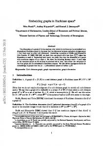
15

2.2. PRELIMINARIES

Figure 2.1: A flat B-scroll over a null curve drawn using the parameterization x(s, t) = (s − a4 t, a2 t2 , s + a2 t) with a = 5. The surface can be reconstructed in more than one way as the sum of two curves. Namely, for instance as x(s, t) = 2 3 3 (a ( s3 − 4s ) + a2 t, a s2 , a ( s3 + s4 ) + a2 t), for which the generating curves are drawn √ on the picture on the left and as x(s, t) = (s, a2 t, s ± a2 t), for which the generating curves are shown on the surface on the right.

2.2.3

Curvatures of translation surfaces

Performing patch computations, the Gaussian curvature, the mean curvature, the second Gaussian curvature and the second mean curvature are calculated for the translation surfaces parameterized by (2.2), (2.3), (2.4) and (2.5). For a surface parameterized by x(s, t) = (s, t, f (s) + g(t)) in Euclidean 3-space the curvatures are given by K=

f ′′ g ′′

2 (1 + f ′2 + g ′2 )

(1 + f ′2 + g ′2 ) ( f ff′′ + ′

KII =

HII =

1

3 2

(1 + f ′2 ) g ′′ + (1 + g ′2 ) f ′′ 2 (1 + f ′2 + g ′2 ) 2 3

g′ g′′′ ) + 2 (1 − f ′2 g′′

+ g ′2 ) f ′′ + 2 (1 + f ′2 − g ′2 ) g ′′

4 (1 + f ′2 + g ′2 ) 2

{(1 + f ′2 + g ′2 ) ( 2

8 (1 + f ′2 + g ′2 )

−4 (1 + f ′2 + g ′2 ) (

′′′

H=

3

2f ′′f (4) − 3f ′′′2 2g ′′ g (4) − 3g ′′′2 + ) f ′′3 g ′′3

f ′ f ′′′ g ′ g ′′′ + ′′ ) + 4 (2f ′2 − g ′2 − 1) f ′′ + 4 (2g ′2 − f ′2 − 1) g ′′ } . f ′′ g

16


The curvatures of a surface parameterized by x(s, t) = (s, t, f (s) + g(t)) in Minkowski 3-space are given by f ′′ g ′′

2

H=

(f ′2 + g ′2 − 1) ( f ff′′ +

g′ g′′′ ) + 2 (g ′2 g′′

K=−

(f ′2 + g ′2 − 1) ′

KII =

HII =

1

′′′

8 ∣f ′2 + g ′2 − 1∣

+4 (f ′2 + g ′2 − 1) (

2 ∣f ′2 + g ′2 − 1∣ 2

3

− f ′2 − 1) f ′′ + 2 (f ′2 − g ′2 − 1) g ′′

4 ∣f ′2 + g ′2 − 1∣ 2

{(f ′2 + g ′2 − 1) ( 2

3 2

(1 − f ′2 ) g ′′ + (1 − g ′2 ) f ′′ 3

3f ′′′2 − 2f ′′f (4) 3g ′′′2 − 2g ′′ g (4) + ) f ′′3 g ′′3

f ′ f ′′′ g ′ g ′′′ + ′′ ) + 4 (g ′2 − 2f ′2 − 1) f ′′ + 4 (f ′2 − 2g ′2 − 1) g ′′ } . f ′′ g

For a surface parameterized by x(s, t) = (f (s) + g(t), s, t) in Minkowski 3-space one has K=−

f ′′ g ′′

2 (1 + f ′2 − g ′2 )

(1 + f ′2 − g ′2 ) ( f ff′′ − ′

KII =

HII =

1

′′′

H=

8 ∣1 + f ′2 − g ′2 ∣

+4 (1 + f ′2 − g ′2 ) (

2 ∣1 + f ′2 − g ′2 ∣ 2

3

g′ g′′′ ) + 2 (1 − f ′2 g′′

− g ′2 ) f ′′ − 2 (1 + f ′2 + g ′2 ) g ′′

4 ∣1 + f ′2 − g ′2 ∣ 2

{(1 + f ′2 − g ′2 ) ( 2

3 2

(1 + f ′2 ) g ′′ + (g ′2 − 1) f ′′ 3

3f ′′′2 − 2f ′′f (4) 3g ′′′2 − 2g ′′ g (4) + ) f ′′3 g ′′3

f ′ f ′′′ g ′ g ′′′ − ′′ ) + 4 (1 − 2f ′2 − g ′2 ) f ′′ − 4 (1 + f ′2 + 2g ′2 ) g ′′ } . f ′′ g

Finally, for a surface in Minkowski 3-space parameterized by x(s, t) = (s + t, g(t), f (s) + t) the curvatures are K=−

KII =

(f ′ − 1) f ′′ g ′ g ′′

((f ′ − 1) + (f ′2 − 1) g ′2 ) 2

2

1 4 ∣(f ′ − 1) + (f ′2 − 1) g ′2 ∣ 2

H=

2

2 ∣(f ′ − 1) + (f ′2 − 1) g ′2 ∣ 2

{− ((f ′ − 1) + (f ′2 − 1) g ′2 ) ( 2

3 2

f ′′ g ′3 − (1 + f ′ ) (1 − f ′ ) g ′′

f ′′′ ′ g f ′′

3 2

17

2.2. PRELIMINARIES + (f ′ − 1)

g ′′′ ) g ′ g ′′

+5 (f ′ − 1) (f ′ + 1) g ′′ + 3 (f ′ − 1) f ′′ g ′ + (3f ′ − 1) f ′′ g ′3 + (f ′ − 1) 2

HII =

3

1

g ′′ } g ′2

{−4 (f ′ − 1) f ′′ 3

8 (f ′ − 1) g ′ ∣(f ′ − 1) + (f ′2 − 1) g ′2 ∣ 2

3 2

+ 8 (f ′ − 1) (f ′ + 1) g ′ g ′′ + 4 (f ′ − 1) (1 − 2f ′) f ′′ g ′2 3

2

+ 4 (f ′ − 1) (−f ′2 + f ′ − 1) f ′′ g ′4 − 4 (f ′ − 1) (f ′ + 1) g ′3 g ′′ 2

+ 4 (f ′ − 1) ((f ′ − 1) + (f ′2 − 1) g ′2 ) ( 2

− ((f ′ − 1) + (f ′2 − 1) g ′2 ) ( 2

2

g ′2 g ′′′ f ′ f ′′′ ′2 (f ′ − 1) f ′′′ ′ g + + (f + 1) ) f ′′ f ′′ g ′′

2g ′ g ′′2 g ′′′ + 2g ′2 g ′′ g (4) − g ′′4 − 3g ′2 g ′′′2 g ′ g ′′3

2 (f ′ − 1) f ′′ f (4) + 2 (f ′ − 1) f ′′2 f ′′′ − f ′′4 − 3 (f ′ − 1) f ′′′2 )} . (f ′ − 1)f ′′3 2

+

2

2

Remark that, in order for a surface parameterized by (2.5) to be non-degenerate, f ′ must be distinct from 1. As mentioned before, in order to be able to define KII and HII for a surface, the surface must not contain points in which K = 0, otherwise the second fundamental form is degenerate. The flat translation surfaces are examined in the next section, but, from the expressions for K it is already clear one needs f ′′ ≠ 0 and g ′′ ≠ 0 if one wants to define KII and HII .

2.2.4

Lambert W-function

When solving a differential equation, it is not always possible to give an explicit solution in terms of elementary functions. Therefore, one makes use of special functions to state solutions of a differential equation. For example, the Legendre’s elliptic integrals describe the surfaces of revolution with constant positive Gaussian curvature, see [74] and an illustration in [36]. In order to solve certain differential equations in the section on the constant curvature translation surfaces, the Lambert W-function turns out to be of great use.

18


Definition 2.6. The Lambert W-function is the multivalued inverse of the function x ↦ xex and is denoted with W . Equivalently, one can say that W (z) has to satisfy W (z)eW (z) = z. The Lambert W-function is implicitly elementary, that is, it is implicitly defined by an equation containing only elementary functions. However, the Lambert Wfunction itself is not an elementary function.

For real x, the Lambert W-function has two real branches, figure 2.2. The principal branch, W0 , is defined for − 1e ≤ x < +∞ and takes on values in [−1, +∞[. The nonprincipal branch, W−1 , is defined for − 1e ≤ x < 0 and has values in [−1, −∞[.

Figure 2.2: The real branches of the Lambert W-function. In 1758 J. H. Lambert gave a series solution of the trinomial equation xm + px = q for x. L. Euler transformed this equation into the more symmetrical form xα −xβ = (α − β)vxα+β which led him to the series solution of the transcendental equation x ln x = v and thereby to the first occurrence of what is now called the Lambert W-function. Sir E. M. Wright contributed to the study of the Lambert W-function and gave several applications of it in the first half of the 20th century. In the 1980s the Lambert W-function is implemented in Maple because its interface required an explicit notation for solutions of equations. For a discussion of the branches and asymptotics of the Lambert W-function as well as applications in combinatorics, iterated exponentiation, solutions of equations, solutions of problems in physics and calculus properties of the Lambert W-function, see [18]. The following lemma states relations between the logarithmic function and the inverse hyperbolic functions. These relations are used to rewrite solutions of differential equations.

2.3. CONSTANT CURVATURE TRANSLATION SURFACES

19

Lemma 2.3. The following relations between the logarithmic function and the inverse hyperbolic functions are valid, 1. 2. 3.

4.

2.3

arcsinh(y) = ln (y +

arccosh(y) = ln (y + 2 arcth(y) = ln (

2 arccoth(y) = ln (

√ 1 + y2) ,

√ y 2 − 1)

1+y ) 1−y

y+1 ) y−1

with y ≥ 1,

with − 1 < y < 1, with − 1 > y or y > 1.

Constant curvature translation surfaces

In this section, translation surfaces for which K, H, KII or HII is a constant, are considered. Parameterizations (2.2), (2.3) and (2.4) are, apart from a possible difference in sign, symmetric in s and t, while (2.5) is not. Since the computations for all parameterizations are similar, only those for (2.3) are given explicitly to save space. The computations for the parameterization (2.5) are given explicitly in the cases where the lack of symmetry in the problem requires adjustments of the methods used. The results, however, are mentioned for all the parameterizations.

2.3.1

Constant Gaussian curvature translation surfaces

The classification of flat translation surfaces follows directly. As shown in [60] for surfaces parameterized by (2.2), (2.3) and (2.4), there exist no such surfaces with non-zero constant Gaussian curvature. Theorem 2.1 ([60]). A translation surface parameterized by x(s, t) = (s, t, f (s) + g(t)) in Euclidean 3-space or a translation surface parameterized by x(s, t) = (s, t, f (s) + g(t)) or x(s, t) = (f (s) + g(t), s, t) in Minkowski 3-space has constant Gaussian curvature if and only if it is (a part of ) a plane or a generalized cylinder and thus, is a flat surface.

20


Theorem 2.2. A translation surface parameterized by x(s, t) = (s + t, g(t), f (s) +t) in Minkowski 3-space has constant Gaussian curvature if and only if it is (a part of ) a plane, a generalized cylinder or a flat B-scroll over a null curve and hence, is a flat surface. Proof. A surface in Minkowski 3-space parameterized by x(s, t) = (s + t, g(t), f (s) +t) has Gaussian curvature K =−

((f ′

(f ′ − 1)f ′′g ′ g ′′ . − 1)2 + (f ′2 − 1)g ′2 )2

(2.8)

Thus K = 0 if and only if f ′′ = 0, g ′ = 0 or g ′′ = 0.

If f ′′ = 0 and g ′′ = 0, the surface is a plane or a flat B-scroll over a null curve if f (s) = −s + a with a ∈ R or g(t) = 0. Remark that f (s) cannot be equal to s + a since that implies the surface is degenerate.

If one of f ′′ and g ′′ is zero and the other is non-zero, the surface is a generalized cylinder or a flat B-scroll over a null curve. Also, if g ′ = 0, the surface is either a plane, a generalized cylinder or a flat B-scroll over a null curve. If one assumes K is a non-zero constant, a contradiction is obtained. Indeed, take the partial derivative with respect to t of equation (2.8) and simplify it to (g ′′2 + g ′ g ′′′ ) (f ′ − 1 + (f ′ + 1)g ′2 ) − 4 (f ′ + 1) g ′2 g ′′2 = 0.

(2.9)

Take the partial derivative with respect to s of the result. Then g ′ g ′′′ =

3g ′2 − 1 ′′2 g . 1 + g ′2

(2.10)

Equations (2.9) and (2.10) lead to a contradiction. Thus, the parameterizations of the statement are found. Conversely, it is clear that the surfaces in the statement have zero Gaussian curvature.

2.3.2

Constant mean curvature translation surfaces

Minimal translation surfaces Minimal translation surfaces in Euclidean 3-space were studied by H. F. Scherk in 1830 as solution to a price question, [77] and [89]. Since the Monge-Legendre equation did not lead to new minimal surfaces, the Jablonowski Society of Leipzig ordered a precise investigation of the Lagrange equation. The Lagrange equation


21

lies at the core of the study of minimal surfaces and by making a thorough study of it, H. F. Scherk found two new minimal surfaces, one of which is now called the minimal translation surface of Scherk. A classification of minimal translation surfaces in Minkowski 3-space is given in [85] for parameterization (2.3) and later also in [60] for parameterizations (2.3) and (2.4). In the latter however, the planes, one Scherk-alike surface and the B-scrolls are missing. Theorem 2.3 ([77]). A translation surface in Euclidean 3-space parameterized by x(s, t) = (s, t, f (s) + g(t)) is a minimal surface if and only if it is (a part of ) a plane or a surface of Scherk which is parameterized by x(s, t) = (s, t,

cos(at) 1 ln ∣ ∣) a cos(as)

with a ∈ R0 .

Figure 2.3: Left: The well-known minimal translation surface of Scherk that is defined on a checker board type of domain. Right: One of the pieces of the minimal translation surface of Scherk with level curves and generating curves displayed on it. Theorem 2.4 ([85]). A spacelike surface in Minkowski 3-space parameterized by x(s, t) = (s, t, f (s) + g(t)) has mean curvature zero if and only if it is (a part of ) either 1. a spacelike plane, 2. the surface of Scherk of the first kind which is parameterized by x(s, t) = (s, t,

1 cosh(at) ln ∣ ∣) a cosh(as)

with tanh2 (as) + tanh2 (at) < 1 and a ∈ R0 .

22


A timelike surface in Minkowski 3-space parameterized by x(s, t) = (s, t, f (s)+g(t)) has mean curvature zero if and only if it is (a part of ) either 1. a timelike plane, 2. the surface of Scherk of the first kind which is parameterized by x(s, t) = (s, t,

cosh(at) 1 ln ∣ ∣) a cosh(as)

with tanh2 (as) + tanh2 (at) > 1 and a ∈ R0 ,

3. the surface of Scherk of the second kind which is parameterized by x(s, t) = (s, t,

cosh(at) 1 ln ∣ ∣) a sinh(as)

with s ≠ 0 and a ∈ R0 ,

4. the surface of Scherk of the third kind which is parameterized by x(s, t) = (s, t,

sinh(at) 1 ln ∣ ∣) a sinh(as)

with s ≠ 0, t ≠ 0 and a ∈ R0 ,

5. a flat B-scroll over a null curve.

Figure 2.4: Left: The minimal translation surface of Scherk of the first kind in Minkowski 3-space with a = 1. The surface is colored according to the function sign(tanh2 (as) + tanh2 (at) − 1). Right: The areas on which the surface of Scherk of the first kind is timelike (outside the star shaped figure) and spacelike (inside the star shaped figure). These areas are bounded by the implicitly defined curve tanh2 (as) + tanh2 (at) − 1 = 0.

Theorem 2.5 ([60]). A spacelike surface in Minkowski 3-space parameterized by x(s, t) = (f (s) + g(t), s, t) has mean curvature zero if and only if it is (a part of ) either


23

Figure 2.5: Left: The minimal translation surface of Scherk of the second kind in Minkowski 3-space with a = 3. Right: The generating curves of the minimal translation surface displayed at the left.

Figure 2.6: Left: The minimal translation surface of Scherk of the third kind in Minkowski 3-space with a = 1.5. Right: The generating curves of the minimal translation surface displayed at the left. 1. a spacelike plane, 2. a surface parameterized by 1 sinh(at) ∣ , s, t) x(s, t) = ( ln ∣ a cos(as)

with a ∈ R0 and tan2 (as) −

1 < 0. sinh2 (at)

24


A timelike surface in Minkowski 3-space parameterized by x(s, t) = (f (s)+g(t), s, t) has mean curvature zero if and only if it is (a part of ) either 1. a timelike plane, 2. a surface parameterized by cosh(at) 1 ∣ , s, t) x(s, t) = ( ln ∣ a cos(as)

with a ∈ R0 ,

3. a surface parameterized by

1 sinh(at) x(s, t) = ( ln ∣ ∣ , s, t) a cos(as)

4. a flat B-scroll over a null curve.

with a ∈ R0 and tan2 (as) −

1 > 0, sinh2 (at)

Figure 2.7: Left: The minimal translation surface in E31 parameterized by x(s, t) = (ln ∣ cos(s)∣ − ln ∣ sinh(t)∣, s, t). Right: The generating curves of the minimal translation surface displayed at the left. Theorem 2.6. A translation surface in Minkowski 3-space parameterized by x(s, t) = (s + t, g(t), f (s) + t) has mean curvature zero if and only if it is (a part of ) either 1. a plane, 2. a flat B-scroll over a null curve,


25

Figure 2.8: Left: One of the pieces of the minimal translation surface in E31 parameterized by x(s, t) = (ln ∣ cos(s)∣ − ln ∣ sinh(t)∣, s, t), colored according to the function sign (tan2 (as) − sinh12 (at) ). Right: The areas on which the minimal surface displayed on the left is timelike (outside the star shaped figures) and spacelike (inside the star shaped figures). These areas are bounded by the implicitly defined curve tan2 (as) − sinh21(at) = 0.

Figure 2.9: Left: The minimal translation surface in E31 parameterized by x(s, t) = (ln ∣ cos(s)∣ − ln ∣ cosh(t)∣, s, t). Right: The generating curves of the minimal translation surface displayed at the left. 3. a surface parameterized by √ ⎞ ⎛ 2t 1 x(s, t) = s + t, ± − , W0 (exp(4as)) − s + t a 2a ⎠ ⎝

(2.11)

26

CHAPTER 2. CONSTANT CURVATURE TRANSLATION SURFACES or by

√ ⎞ ⎛ 2t 1 x(s, t) = s + t, ± − , W0 (− exp(4as)) − s + t a 2a ⎠ ⎝

4. a surface parameterized by √ ⎞ ⎛ 2t 1 x(s, t) = s + t, ± − , W−1 (− exp(4as)) − s + t a 2a ⎠ ⎝

with a ∈ R0 , (2.12)

with a ∈ R0 . (2.13)

Proof. A translation surface parameterized by x(s, t) = (s + t, g(t), f (s) + t) in Minkowski 3-space has mean curvature H=

f ′′ g ′3 − (1 + f ′ )(1 − f ′ )2 g ′′ 2 ∣(f ′ − 1)2 + (f ′2 − 1)g ′2 ∣ 2 3

.

Hence, the mean curvature is zero if and only if f ′′ g ′3 − (1 + f ′ )(1 − f ′ )2 g ′′ = 0.

(2.14)

If f ′ = −1 or g ′ = 0, the surface is a plane or a flat B-scroll over a null curve. For f ′′ = 0 and g ′′ = 0 the surface is a plane or a flat B-scroll over a null curve. Thus, assume f ′′ ≠ 0 and g ′′ ≠ 0. Then, the minimality condition (2.14) can be separated for the variables f ′′ =a (1 − f ′ )2 (1 + f ′ )

and

g ′′ =a g ′3

with a ∈ R0 .

(2.15)

Performing integration by parts, the integrals 1 ′ ∫ (1 − f ′ )2 (1 + f ′ ) df = a ∫ ds

are ln ∣

1 + f′ 2 ∣+ = 4as + b 1 − f′ 1 − f′

with b ∈ R.

(2.16)

But, if the differential equation (2.15) for the function f is multiplied by 1 + f ′ first and then integrated, one has ∫ Therefore,

1 df ′ = a (∫ ds + ∫ df ) . (1 − f ′ )2

1 = as + af + c 1 − f′

with c ∈ R

2.3. CONSTANT CURVATURE TRANSLATION SURFACES and thus,

27

1 + f′ =

2as + 2af + 2c − 1 . as + af + c With this, equation (2.16) reduces to,

Thus,

ln ∣ 2as + 2af (s) + 2c − 1 ∣ + 2as + 2af (s) + 2c − 1 = 4as + b − 1

∣ 2as + 2af (s) + 2c − 1 ∣ exp(2as + 2af (s) + 2c − 1) = exp(4as + b − 1).

From the definition of the Lambert W-function one has

W0 (exp(4as + b − 1)) = 2as + 2af (s) + 2c − 1,

for 2as + 2af (s) + 2c − 1 > 0 and or

W0 (− exp(4as + b − 1)) = 2as + 2af (s) + 2c − 1,

W−1 (− exp(4as + b − 1)) = 2as + 2af (s) + 2c − 1,

for 2as + 2af (s) + 2c − 1 < 0. Hence, or

f (s) =

f (s) =

c 1 1 W0 (± exp(4as + b − 1)) − s − + 2a a 2a

c 1 1 W−1 (− exp(4as + b − 1)) − s − + . 2a a 2a

From equation (2.15), the solution for the function g is √ −2at + d g(t) = ∓ + m with d, m ∈ R. a Therefore, possibly after applying a transformation, the parameterizations stated in the theorem follow. Conversely, it is verified easily that the surfaces of the statement are minimal. Remark. The flat B-scrolls and surfaces parameterized by (2.12) or (2.13) are timelike and surfaces parameterized by (2.11) have a spacelike and a timelike part. The three non-plane surfaces of Theorem 2.6 are implicitly described by the equation 2a (x + ay 2 + z) exp (2az − 2ax) ± 1 = 0.

(2.17)

When the plus sign is chosen one finds the surfaces parameterized by (2.12) and (2.13) and the minus sign describes the surfaces parameterized by (2.11). This implicit description of these surfaces provides much better visualizations of the surfaces, see figure 2.10.

28


Figure 2.10: Left: The minimal translation surface parameterized by (2.17) with a = −1 and the plus sign. Right: The minimal translation surface parameterized by (2.17) with a = −1 and the minus sign. CMC translation surfaces A classification of constant mean curvature translation surfaces parameterized by (2.2), (2.3) or (2.4) is given in [60]. Theorem 2.7 ([60]). A surface in Euclidean 3-space parameterized by x(s, t) = (s, t, f (s) + g(t)) has non-zero constant mean curvature H if and only if it is (a part of ) a cylinder parameterized by √ 1 + a2 √ x(s, t) = (s, t, as ± 1 − 4H 2 t2 ) with a ∈ R. 2H Theorem 2.8 ([60]). A spacelike surface parameterized by x(s, t) = (s, t, f (s) + g(t)) in Minkowski 3-space has non-zero constant mean curvature H if and only if it is (a part of ) a cylinder parameterized by √ 1 − a2 √ 1 + 4H 2 t2 ) with a ∈ R and ∣a∣ < 1. x(s, t) = (s, t, as ± 2H

A timelike surface in Minkowski 3-space parameterized by x(s, t) = (s, t, f (s)+g(t)) has non-zero constant mean curvature H if and only if it is (a part of ) either

2.3. CONSTANT CURVATURE TRANSLATION SURFACES 1. a cylinder parameterized by √ a2 − 1 √ 1 − 4H 2 t2 ) x(s, t) = (s, t, as ± 2H 2. a cylinder parameterized by √ 1 − a2 √ 2 2 4H t − 1) x(s, t) = (s, t, as ± 2H

29

with a ∈ R and ∣a∣ > 1, with a ∈ R and ∣a∣ < 1.

Remark that in Theorems 2.7 and 2.8 the role of s and t can of course be reversed. Theorem 2.9 ([60]). A spacelike surface parameterized by x(s, t) = (f (s) + g(t), s, t) in Minkowski 3-space has non-zero constant mean curvature H if and only if it is (a part of ) either 1. a cylinder parameterized by √ 1 + a2 √ 2 2 x(s, t) = (as ± 4H t − 1, s, t) 2H

2. a cylinder parameterized by √ a2 − 1 √ 1 + 4H 2 s2 + at, s, t) x(s, t) = (± 2H

with a ∈ R,

with a ∈ R and ∣a∣ > 1.

A timelike surface in Minkowski 3-space parameterized by x(s, t) = (f (s)+g(t), s, t) has non-zero constant mean curvature H if and only if it is (a part of ) either 1. a cylinder parameterized by √ 1 + a2 √ 1 + 4H 2 t2 , s, t) x(s, t) = (as ± 2H

2. a cylinder parameterized by √ 1 − a2 √ 1 − 4H 2 s2 + at, s, t) x(s, t) = (± 2H 3. a cylinder parameterized by √ a2 − 1 √ 2 2 4H s − 1 + at, s, t) x(s, t) = (± 2H

with a ∈ R,

with a ∈ R and ∣a∣ < 1, with a ∈ R and ∣a∣ > 1.

30


Similar results are valid for surfaces parameterized by (2.5). Theorem 2.10. A surface parameterized by x(s, t) = (s + t, g(t), f (s) + t) in Minkowski 3-space has non-zero constant mean curvature H if and only if it is (a part of ) either 1. a cylinder parameterized by x(s, t) = (s + t, at,

√ a s ± 4a2 H 2 s2 − a2 − 1 + t) a2 + 1 2(a2 + 1)H

with a ∈ R,

2. a cylinder parameterized by x(s, t) = (s + t, at,

a2

√ a s ± 4a2 H 2 s2 + a2 + 1 + t) 2 + 1 2(a + 1)H

with a ∈ R. (2.18)

3. a cylinder parameterized by x(s, t) = (s + t,

√ ±1 (1 + a)2 + 4H 2 (1 − a2 )t2 , as + t) with a ∈ R, a ≠ −1. 2(a + 1)H

x(s, t) = (s + t,

√ ±1 4(1 − a2 )H 2 t2 − (1 + a)2 , as + t) with a ∈ R, a ≠ −1. 2(a + 1)H

4. a cylinder parameterized by

Proof. Assume first f ′′ ≠ 0 and g ′′ ≠ 0. Take the partial derivative of the constant mean curvature 2 f ′′ g ′3 − (1 + f ′ ) (1 − f ′ ) g ′′ H= 3 2 2 2 ∣(f ′ − 1) + (f ′2 − 1) g ′2 ∣ with respect to t and simplify. This results in

3f ′′g ′2 g ′′ − (f ′ + 1)(f ′ − 1)2 g ′′′ + (f ′ + 1)2 (f ′ − 1)(3g ′g ′′2 − g ′2 g ′′′) = 0. (2.19)

Divide equation (2.19) by (f ′ + 1)2 (f ′ − 1) and differentiate the result with respect to s. Then, ( (f ′ +1)f2 (f ′ −1) )

′

′′

3

( ff ′ −1 ) +1 ′

′

=

g ′′′ =a g ′2 g ′′

with a ∈ R


31

if one assumes g ′′ ≠ 0. Thus g ′′′ = ag ′2 g ′′ and g ′′ = a3 g ′3 + b with b ∈ R. With this, equation (2.19) is simplified and if the partial derivative with respect to t is taken, 3f ′′ = a(f ′ + 1)(f ′ − 1)2 .

But, if this is used in the simplified equation (2.19) it turns out that b = 0. Because 3f ′′ = a(f ′ + 1)(f ′ − 1)2 and g ′′ = a3 g ′3 imply H = 0, a contradiction is the result.

Therefore, f ′′ = 0 or g ′′ = 0.

Assume first g ′′ = 0 and g(t) = at + b with a, b ∈ R, a ≠ 0. Hence, H=

a3 f ′′

2∣a2 (f ′2 − 1) + (f ′ − 1)2 ∣ 2 3

(2.20)

.

For a2 (f ′2 − 1) + (f ′ − 1)2 > 0 equation (2.20) is rewritten to (a2 (f ′2

which is equivalent with

(−

It follows f′ =

a2

a4

− 1) + (f ′

3 − 1)2 ) 2

a2 f ′ + f ′ − 1

f ′′ = 2aH,

′

1 ) = 2aH.

(a2 (f ′2 − 1) + (f ′ − 1)2 ) 2

a2 −2aHs + c 1 ± 2 √ + 1 (a + 1) −a2 − 1 + (2aHs + c)2

with c ∈ R

if (2aHs + c)2 > 1 + a2 . Hence, f (s) =

√ s a ∓ −a2 − 1 + (2aHs + c)2 + d a2 + 1 2(a2 + 1)H

with d ∈ R.

For a2 (f ′2 − 1) + (f ′ − 1)2 < 0 equation (2.20) is solved similar, the result is √ s a f (s) = 2 ± a2 + 1 + (2aHs + c)2 + d with d ∈ R. 2 a + 1 2(a + 1)H If f ′′ = 0 and f (s) = as + b with a, b ∈ R and a ≠ ±1, the mean curvature is H=

−(1 + a)(1 − a)2 g ′′

2∣ (a − 1)2 + (a2 − 1)g ′2 ∣ 2 3

.

For (a − 1)2 + (a2 − 1)g ′2 > 0 equation (2.21) is equivalent with (

−(1 + a)g ′

′

1 ) = 2H.

((a − 1)2 + (a2 − 1)g ′2 ) 2

(2.21)

32 Thus,


g(t) = ±

√ 1 (1 + a)2 + (1 − a2 )(2Ht + c)2 + d. 2(a + 1)H

For (a − 1)2 + (a2 − 1)g ′2 < 0 equation (2.21) is (

′

−(1 + a)g ′

(−(a − 1)2 + (a2 − 1)g ′2 ) 2

1

) = 2H

√ 1 (1 − a2 )(2Ht + c)2 − (1 + a)2 + d. 2(a + 1)H Conversely, it is verified directly that the surfaces in the statement of the theorem have constant mean curvature. and

g(t) = ±

For this classification theorem two remarks are made. Remark. All the surfaces in the statement of theorem 2.10 have a spacelike and a timelike part. Moreover, it are all cylinders since, in the first two parameterizations, the rulers are (t, at, t) and in the last two parameterizations, the rulers are (s, 0, as).

Figure 2.11: Left: CMC translation surface in Minkowski 3-space parameterized by (2.18) with a = 2 and H = 31 . Right: The generating curves of the surface displayed at the left. Remark. From the preceding theorems, one concludes a translation surface parameterized by (2.2), (2.3), (2.4) or (2.5) with non-zero constant mean curvature is a generalized cylinder and thus a flat surface. That is, for translation surfaces H equal to a non-zero constant implies that K is zero.


2.3.3

33

Constant second Gaussian curvature translation surfaces

In this section, a characterization theorem for II-flat translation surfaces is proved. Thereafter, it is shown there exist no translation surfaces with KII equal to a nonzero constant. Part of these results appeared in [35]. II-flat translation surfaces As pointed out in [13], for a surface in Euclidean 3-space, minimality implies II-flatness but not vice versa. The incorrectness of the converse statement is illustrated with an example of a translation surface which is II-flat but not minimal, namely the surface parameterized by 4 3 1 4 x(s, t) = (s, t, c 3 (s 3 − t 3 )) . 4 This surface is also found in [70] and [72] in which f (s) and g(t) may contain fractional powers of s and t, respectively, and the II-flat surfaces are classified. This translation surface is one special instance of the characterization given in the next theorem, namely, take the constants a and b zero and assume the constant c is non-zero.

Theorem 2.11. A translation surface parameterized by x(s, t) = (s, t, f (s) + g(t)) in Euclidean 3-space has second Gaussian curvature equal to zero, if and only if f (s) = ∫ F −1 (s + d) ds

and

with F and G real functions determined by F (x) = ∫

ax4

x2 dx + bx2 + c

and

G(x) = ∫

g(t) = ∫ G−1 (t + m) dt −ax4

and a, b, c, d and m real numbers.

x2 dx + (−2a + b)x2 − a + b − c

Apart from some sign differences the characterization of II-flat translation surfaces in E31 parameterized by (2.3) or (2.4) is the same.

Theorem 2.12. A translation surface parameterized by x(s, t) = (s, t, f (s) + g(t)) in Minkowski 3-space has second Gaussian curvature equal to zero if and only if f (s) = ∫ F −1 (s + d) ds

and


x2 dx ax4 + bx2 + c

and


g(t) = ∫ G−1 (t + m) dt

G(x) = ∫

x2 dx −ax4 + (2a + b)x2 − a − b − c

34


Proof. The second Gaussian curvature of a surface parameterized by x(s, t) = (s, t, f (s) + g(t)) in Minkowski 3-space is given by (f ′2 + g ′2 − 1) ( f ff′′ + ′

KII =

′′′

g′ g′′′ ) + 2 (g ′2 g′′

− f ′2 − 1) f ′′ + 2 (f ′2 − g ′2 − 1) g ′′

4 ∣f ′2 + g ′2 − 1∣ 2

3

.

Thus the second Gaussian curvature is zero if and only if (f ′2 + g ′2 − 1) (

f ′ f ′′′ g ′ g ′′′ + ′′ )+2 (g ′2 − f ′2 − 1) f ′′ +2 (f ′2 − g ′2 − 1) g ′′ = 0 (2.22) f ′′ g

Take the partial derivative with respect to s and t of equation (2.22) and simplify the result. This yields two differential equations ′

2f ′′2 + f ′ f ′′′ ( ) = af ′ f ′′ f ′′

′

and

2g ′′2 + g ′ g ′′′ ( ) = −ag ′ g ′′ g ′′

with a ∈ R.

Each of these equations can be integrated twice. After rewriting the integration constants, one has f ′2 f ′′ = af ′4 +bf ′2 +c and g ′2 g ′′ = −ag ′4 +pg ′2 +q, with a, b, c, p, q ∈ R. Use this in equation (2.22), then p = 2a + b and q = −a − b − c. Consequently, one has to solve the differential equations f ′2 f ′′ = af ′4 + bf ′2 + c

and

g ′2 g ′′ = −ag ′4 + (2a + b)g ′2 − a − b − c

(2.23)

with a, b, c ∈ R. These equations can be integrated. From f ′2 f ′′ = 1 af ′4 + bf ′2 + c

it follows f (s) = ∫ F −1 (s + d) ds with F (x) = ∫

ax4

x2 dx. + bx2 + c

The equation for the function g is integrated similar. Hence, the statement of the theorem follows. Theorem 2.13. A translation surface in Minkowski 3-space parameterized by x(s, t) = (f (s) + g(t), s, t) has second Gaussian curvature equal to zero if and only if f (s) = ∫ F −1 (s + d) ds and g(t) = ∫ G−1 (t + m) dt


x2 dx ax4 + bx2 + c

and


G(x) = ∫

−ax4

x2 dx + (2a − b)x2 − a + b − c

35


In line with the expectations the characterization of II-flat translation surfaces parameterized by (2.5) in E31 is of the same genre but nevertheless somewhat different. Theorem 2.14. A translation surface in Minkowski 3-space parameterized by x(s, t) = (s + t, g(t), f (s) + t) has second Gaussian curvature equal to zero if and only if f (s) = ∫ F −1 (s + d) ds and g(t) = ∫ G−1 (t + m) dt

with F and G real functions determined by

and

F (x) = ∫

(−a + b − c)x3

1 dx + (3a − b − c)x2 + (−3a − b + c)x + a + b + c

G(x) = ∫

1 dx ax5 + bx3 + cx

and a, b, c, d and m real numbers. Proof. The second Gaussian curvature of a surface parameterized by x(s, t) = (s + t, g(t), f (s) + t) is zero if and only if (−(f ′ − 1)2

f ′′′ ′3 f ′′′ ′ ′′ ′ ′ ′′ ′2 + 3(f − 1)f ) g + ((3f − 1)f − (f − 1) )g f ′′ f ′′

(f ′ − 1) ( 3

g ′′ g ′′′ g ′ g ′′′ ′ 2 ′ ′′ − ) + (f − 1) (f + 1) (5g − ) = 0. (2.24) g ′2 g ′ g ′′ g ′′

Divide this by (f ′ −1)3 g ′3 and take the derivative with respect to s and t. Carrying out these steps separates the variables and one arrives at g ′3 5g ′′2 − g ′ g ′′′ (f ′ − 1)2 3f ′′2 − (f ′ − 1)f ′′′ ( ) = − ( ) = a. f ′′ (f ′ − 1)2 f ′′ g ′′ g ′3 g ′′ ′

′

Integrate these equations

a f ′′ = − (f ′ − 1) + b(f ′ − 1)2 + c(f ′ − 1)3 2 g ′′ =

a ′ d ′3 g + g + mg ′5 . 8 2

Combining this with equation (2.24) leads to d = a2 + b and m = the statement of the theorem follows by integrating g ′′ = ag ′5 + bg ′3 + cg ′

a 8

+

b 2

− c. Hence, (2.25)

36


and f ′′ = a + b + c + (−3a − b + c)f ′ + (+3a − b − c)f ′2 + (−a + b − c)f ′3 ,

(2.26)

which are found after renaming the constants.

Remark. As calculated in Lemma 2.2, the implication H = 0 ⇒ KII = 0 is valid for surfaces in E31 . But that means the minimal translation surfaces must be incorporated in the characterization of Theorems 2.12, 2.13 and 2.14. Indeed, if b = −a ≠ 0 and c = 0 in equations (2.23), these reduce to the differential equations that describe the minimal surfaces parameterized by (2.4). Analogously, if a = 0 = c and b ≠ 0 in equations (2.25) and (2.26), the differential equations characterize the minimal surfaces parameterized by (2.5). For other special choices of the constants, the differential equations which determine the functions f and g of a II-flat translation surface, can be solved. Hence, in these cases, an explicit parameterization of the surfaces can be given. Some specific solutions of the differential equations f ′2 f ′′ = af ′4 + bf ′2 + c and g ′2 g ′′ = −ag ′4 + (2a + b)g ′2 − a − b − c of Theorem 2.12 Case a = 0, b = 0 and c ≠ 0

After applying appropriate transformations the surface is parameterized by x(s, t) = (

s 3 t3 1 4 4 , − , (s − t )) . 3c 3c 4c

(2.27)

The Euclidean equivalent of this surface is given in [13] as example of a II-flat but non-minimal surface. Case a = 0, b ≠ 0 and c = 0 The differential equation for the function g is g ′′ −

g ′′ = b. 1 − g ′2

(2.28)

Integrate equation (2.28) using partial fractions, then g′ +

1 1 − g′ ln ∣ ∣ = bt + n 2 1 + g′

with n ∈ R.

(2.29)

37


But, from equation (2.29) the function g ′ cannot be solved immediately. Multiply equation (2.28) with g ′ and integrate, g ′2 1 + ln ∣1 − g ′2 ∣ = bg + p˜ 2 2

with p˜ ∈ R.

This equation is equivalent to

∣1 − g ′2 ∣ exp (g ′2 − 1) = exp (2bg + p)

For g ′2 < 1 this is rewritten

with p ∈ R.

(g ′2 − 1) exp(g ′2 − 1) = − exp(2bg + p).

Hence, using the definition of the Lambert W-function,

g ′2 (t) − 1 = W0 (− exp(2bg(t) + p)).

√ g ′ (t) = ± 1 + W0 (− exp (2bg(t) + p)).

Thus,

The choice for the principal branch is necessary for the function g ′ to be realvalued. Similar, if g ′2 > 1 one has

√ g ′ (t) = ± 1 + W0 (exp (2bg(t) + p)).

Use these results for g ′ in equation (2.29). Then the function g is implicitly defined by √ √ ± 1 + W0 (− exp (2bg(t) + p)) ∓ arcth 1 + W0 (− exp (2bg(t) + p)) = bt + n

or by

√ √ ± 1 + W0 (exp (2bg(t) + p)) ∓ arccoth 1 + W0 (exp (2bg(t) + p)) = bt + n.

After applying appropriate transformations the surfaces are parameterized by x(s, t) = (s,

√ 1 √ b (± 1 + W0 (− exp (2bt)) ∓ arcth 1 + W0 (− exp (2bt))) , s2 + t) b 2

with 2bt < −1 or x(s, t) = (s,

(2.30)

√ b 1 √ (± 1 + W0 (exp (2bt)) ∓ arccoth 1 + W0 (exp (2bt))) , s2 + t) . b 2

38


Figure 2.12: Left: Translation surface parameterized by (2.27) with c = 2.5. Right: Translation surface parameterized by (2.30) with b = 1.5. Case a ≠ 0, b = 0 and c = 0 The differential equations can be solved as demonstrated above. After applying appropriate transformations one obtains 1 x(s, t) = (s, (± arcth 2a

√ 1+

±W−1 (− exp (2at))

with 2at < −1 or

1 x(s, t) = (s, (± arccoth 2a

1 W−1 (− exp (2at))

√ 1+

√ 1+

1 1 ) , − ln ∣as∣ + t) W−1 (− exp (2at)) a

1 W0 (exp (2at))

√ ±W0 (exp (2at)) 1 +

Case a = 0, b ≠ 0 and c ≠ 0

(2.31)

1 1 ) , − ln ∣as∣ + t) . W0 (exp (2at)) a

The subcase b = −c is analogous to the case where only the constant b is nonzero, but with the role of the functions f and g reversed. For the subcase b ≠ −c


39

one solves the differential equations as above but one must take into account the signs of bc and b(b + c). For instance, for bc > 0 and b(b + c) > 0 the surfaces are parameterized by ⎛1 x(s, t) = ⎝b

√

√ c⎛ 2b2 s)) ± −1 − W−1 (− exp (− b⎝ c ∓ arctan

1 b

√

√

−1 − W−1 (− exp (−

√ b+c ⎛ 2b2 t)) ± 1 + W0 (− exp ( b ⎝ b+c ∓ arcth

with

2b2 c

s > 1 and

⎛1 x(s, t) = ⎝b

2b2 b+c

√

t < −1 and

1 + W0 (− exp (

√ c⎛ 2b2 s)) ± −1 − W−1 (− exp (− b⎝ c ∓ arctan

1 b

√

√

√

−1 − W−1 (− exp (−

√ b+c ⎛ 2b2 t)) ± 1 + W0 (exp (− b ⎝ b+c ∓ arccoth

⎞ 2b2 s)) , c ⎠

√

⎞ ⎞ 2b2 t)) , s + t . b+c ⎠ ⎠

⎞ 2b2 s)) , c ⎠

1 + W0 (exp (−

⎞ ⎞ 2b2 t)) , s + t b+c ⎠ ⎠

with 2bc s > 1. Similar parameterizations are found for other combinations of the signs of bc and b(b +c). Remark that the combination bc > 0 and b(b +c) < 0 cannot occur. 2

For other choices of the constants it is not always possible to solve the differential equations for an explicit expression of the functions f and g. Using maple, numerical solutions can be given, see for example figure 2.13 at the right.

40


Figure 2.13: Left: Translation surface parameterized by (2.31) with a = 1.8. Right: General solution of the differential equations (2.23) with a = 1, b = 7, c = − 41 and initial values f (0) = 0, f ′ (0) = 12 , g(0) = 0 and g ′ (0) = 2. Some specific solutions of the differential equations f ′′ = a + b + c + (−3a − b + c)f ′ + (3a − b − c)f ′2 + (−a + b − c)f ′3 and g ′′ = ag ′5 + bg ′3 + cg ′ of Theorem 2.14 Case a ≠ 0, b = 0 and c = 0 Surfaces parameterized by x(s, t) = (s + t, ±

have vanishing KII .

3 1√ 1 (−4at) 4 , s ± 2as + t) , 3a a

(2.32)

Case a = 0, b ≠ 0 and c = 0 As pointed out in a remark above, in this case the differential equations for f and g characterize the minimal translation surfaces parameterized by (2.5).


41

Case a = 0, b = 0 and c ≠ 0 Again, using the Lambert W-function makes it possible to explicitly state the parameterizations x(s, t) = (s + t,

x(s, t) = (s + t,

1 1 exp(ct), W0 (± exp(−4cs)) + s + t) , c 2c

1 1 exp(ct), W−1 (− exp(−4cs)) + s + t) . c 2c These parameterizations can be summarized by the implicit equation 2c(z − x) exp (2c(x + z) − 4 ln ∣cy∣) ± 1 = 0.

(2.33) (2.34)

(2.35)

If the minus sign of (2.35) is chosen, the surfaces parameterized by (2.33), for the plus sign, are reconstructed and with the choice for the plus sign in (2.35), the surfaces parameterized by (2.34) and by (2.33), for the minus sign, are found. For other values of the constants one can proceed similarly, but it is not always possible to give an explicit solution for the functions f and g. For a numerical solution, constructed using Maple, see figure 2.14 at the right.

Figure 2.14: Left: Translation surface parameterized by (2.32) with a = 1.5. Right: General solution of the differential equations (2.23) with a = − 41 , b = 2, c = 13 and initial values f (0) = 0, f ′ (0) = 13 , g(0) = 0 and g ′ (0) = −1.

42


Translation surfaces with non-zero constant KII In contrast with the large class of translation surfaces with vanishing second Gaussian curvature, the non-existence of translation surfaces with constant nonzero second Gaussian curvature is shown. Theorem 2.15. There exists no translation surface in Euclidean 3-space parameterized by x(s, t) = (s, t, f (s) + g(t)) or in Minkowski 3-space parameterized by x(s, t) = (s, t, f (s) +g(t)), x(s, t) = (f (s) + g(t), s, t) or x(s, t) = (s + t, g(t), f (s) + t) with non-zero constant second Gaussian curvature.

Proof. The second Gaussian curvature of a surface in Minkowski 3-space parameterized by x(s, t) = (s, t, f (s) +g(t)) is given by 4KII

=

1

∣f ′2 + g ′2 − 1∣

3 2

+

=

R1

∣f ′2 + g ′2 − 1∣ 2

3

(−4g ′2 g ′′ − 4f ′2 f ′′ + (f ′2 + g ′2 − 1) (

g ′ g ′′′ + 2g ′′2 g ′′

f ′ f ′′′ + 2f ′′2 )) f ′′

(2.36)

.

Take the partial derivative of equation (2.36) with respect to s, then, 0=

1

∣f ′2 + g ′2 − 1∣ 2

3

(−4 (f ′2 f ′′ ) + 2f ′ f ′′ ( ′

′

g ′ g ′′′ + 2g ′′2 f ′ f ′′′ + 2f ′′2 + ) g ′′ f ′′

f ′ f ′′′ + 2f ′′2 3f ′ f ′′ R1 . +(f + g − 1) ( ) ) − 3 f ′′ ∣ f ′2 + g ′2 − 1 ∣ 2 (f ′2 + g ′2 − 1) ′2

′2

Use equation (2.36) in this expression 12KII =

′2 ′′ g ′ g ′′′ + 2g ′′2 f ′ f ′′′ + 2f ′′2 f ′2 + g ′2 − 1 ⎛ (f f ) +2 +2 −4 3 ′ ′′ ′′ ff g f ′′ ∣f ′2 + g ′2 − 1∣ 2 ⎝ ′

1 f ′ f ′′′ + 2f ′′2 R2 (f ′2 + g ′2 − 1) . (2.37) ( ))= 3 ′ ′′ ′′ ff f ∣f ′2 + g ′2 − 1∣ 2 ′

+(f ′2 + g ′2 − 1)

43


Take the partial derivative of equation (2.37) with respect to t and use equation (2.37), then one obtains, 6KII

= ∣f ′2 + g ′2 − 1∣ 2 ( 1

′

′

1 2g ′′2 + g ′ g ′′′ 1 2f ′′2 + f ′ f ′′′ ( ) + ′ ′′ ( )) ′ ′′ ′′ gg g f f f ′′

= ∣f ′2 + g ′2 − 1∣ 2 R3 . 1

(2.38)

Take the partial derivative of equation (2.38) with respect to s and use again equation (2.38), then, −6KII = ∣f ′2 + g ′2 − 1∣ 2 (f ′2 + g ′2 − 1) 1

′ ′

1 1 2f ′′2 + f ′ f ′′′ ( ′ ′′ ( )) . ′ ′′ ff ff f ′′

Finally, take the partial derivative with respect to t of this equation, the contradiction KII = 0 is the result.

For a surface in Minkowski 3-space parameterized by x(s, t) = (s + t, g(t), f (s) + t) the second Gaussian curvature is 4KII =

1

∣(f ′ − 1)2 + (f ′2 − 1)g ′2 ∣ 2 3

((f ′ − 1)3 (

+ (f ′ − 1)2 (f ′ + 1) (5g ′′ −

+

g ′ g ′′′ ) g ′′

g ′′2 − g ′ g ′′′ ) g ′2 g ′′

(f ′ − 1)(3f ′′2 − (f ′ − 1)f ′′′) ′ (3f ′ − 1)f ′′2 − (f ′2 − 1)f ′′′ ′3 g + g ). f ′′ f ′′

Proceed as for the previous parameterization, that is, take twice the partial derivative with respect to t and s and then again with respect to s and t while simplification is executed in between. Then, because of the asymmetry in the variables s and t, take three times the partial derivative with respect to t while simplifying in between. Finally, take the partial derivative with respect to s, the result is a contradiction. In the previous proof, the simplification in between two steps of partial differentiation is important and must be chosen well since every time a partial derivative is taken, the resulting equation must contain at least one term less than the previous equation.

44


2.3.4

Constant second mean curvature translation surfaces

In [63], the question raised in [31], whether there exist in Euclidean 3-space II-minimal translation surfaces constructed as the sum of two planar curves, is answered negatively. This theorem is proved in [70] and in [71]. Here, a proof is given for the non-existence of II-minimal translation surfaces in Minkowski 3space. In [71], examples of II-minimal surfaces in spheres are discussed and the relation between II-minimality and biharmonicity is recalled. Theorem 2.16. There exists no translation surface parameterized by x(s, t) = (s, t, f (s) + g(t)) in Euclidean 3-space or parameterized by x(s, t) = (s, t, f (s) +g(t)), x(s, t) = (f (s) + g(t), s, t) or x(s, t) = (s + t, g(t), f (s) + t) in Minkowski 3-space with constant second mean curvature. Proof. For a surface in Minkowski 3-space parameterized by x(s, t) = (s, t, f (s) +g(t)) the second mean curvature is zero if and only if −3

f ′2 f ′′ + g ′2 g ′′

(f ′2 + g ′2 − 1)

2

+

f ′′2 + f ′ f ′′′ g ′′2 + g ′ g ′′′ 1 ( + ) f ′2 + g ′2 − 1 f ′′ g ′′ −

2f ′′ f (4) − 3f ′′′2 2g ′′ g (4) − 3g ′′′2 − = 0. (2.39) 4f ′′3 4g ′′3

Take the partial derivative of this equation with respect to s. Then, (f ′2 f ′′ ) (f ′2 + g ′2 − 1) − 4 (f ′2 f ′′ + g ′2 g ′′ ) f ′ f ′′ ′

−3

(f ′2 + g ′2 − 1)

3

−

2f ′ f ′′

(f ′2 + g ′2 − 1)

2

(

′

+

1 f ′′2 + f ′ f ′′′ ( ) f ′2 + g ′2 − 1 f ′′ ′

f ′′2 + f ′ f ′′′ g ′′2 + g ′ g ′′′ 2f ′′f (4) − 3f ′′′2 + ) − ( ) = 0. f ′′ g ′′ 4f ′′3 (2.40)

Now, take the partial derivative with respect to t and multiply the result with (f ′2 +g′2 −1)4 . Then, f ′ f ′′ g′ g′′ (g ′2 g ′′ ) ⎞ ⎛ (f ′2 f ′′ ) 6 (f + g − 1) + − 36 (f ′2 f ′′ + g ′2 g ′′ ) g ′ g ′′ ⎠ ⎝ f ′ f ′′ ′

′2

′

′2

+ 4 (f ′2 + g ′2 − 1) (

f ′′2 + f ′ f ′′′ g ′′2 + g ′ g ′′′ + ) f ′′ g ′′

45

2.3. CONSTANT CURVATURE TRANSLATION SURFACES ′

′

f ′′2 + f ′ f ′′′ 1 g ′′2 + g ′ g ′′′ 1 ) + ( ) ] = 0. (2.41) − (f + g − 1) [ ′ ′′ ( ff f ′′ g ′ g ′′ g ′′ ′2

2

′2

Take again the partial derivative with respect to s. This results in ′ ′′ ⎛

12f f

(f ′2 f ′′ )

′

⎝ f ′ f ′′

+ 8f ′ f ′′ (

(g ′2 g ′′ ) ⎞ ⎛ (f ′2 f ′′ ) ⎞ ′ ′2 ′2 (f + − 36 (f ′2 f ′′ ) + 6 + g − 1) ′ ′′ ′ ′′ gg ⎠ ⎠ ⎝ f f ′

′

′

f ′′2 + f ′ f ′′′ f ′′2 + f ′ f ′′′ g ′′2 + g ′ g ′′′ ′2 ′2 (f + ) + 4 + g − 1) ( ) f ′′ g ′′ f ′′

− 4f ′ f ′′ (f ′2 + g ′2 − 1) [

′

′

′

1 f ′′2 + f ′ f ′′′ 1 g ′′2 + g ′ g ′′′ ( ) + ′ ′′ ( )] ′ ′′ ′′ ff f gg g ′′ ′ ′

1 f ′′2 + f ′ f ′′′ − (f + g − 1) [ ′ ′′ ( )] =0 f f f ′′ ′2

′2

2

(2.42)

and take the partial derivative with respect to t and divide by f ′ f ′′ g ′ g ′′ . Then, after simplification, ⎡ ′ ′ ′ ′⎤ ⎥ ⎢ 1 1 f ′′2 + f ′ f ′′′ 1 1 g ′′2 + g ′ g ′′′ ( ( ) ) ( ( ) )⎥ − (f ′2 + g ′2 − 1) ⎢ + ⎥ ⎢ f ′ f ′′ f ′ f ′′ ′′ ′ ′′ ′ ′′ ′′ f gg gg g ⎥ ⎢ ⎦ ⎣

′2 ′′ ′2 ′′ 3 ⎛ (g g ) ⎞ 3 ⎛ (f f ) ⎞ + = 0. (2.43) f ′ f ′′ ⎝ f ′ f ′′ ⎠ g ′ g ′′ ⎝ g ′ g ′′ ⎠ ′

′

′

′

Take a last time the partial derivative with respect to s, that is,

′ ′ ⎤′ ′ ′ ⎡ ⎡ ′′2 ′ ′′′ ′ ⎤ ⎥ ⎢ 3 ⎛ (f ′2 f ′′ ) ⎞ ⎥ ⎢ 1 1 f + f f ′2 ′2 ⎢ ⎥ ⎢ ))⎥ ⎥ ⎢ f ′ f ′′ ⎝ f ′ f ′′ ⎠ ⎥ − (f + g − 1) ⎢ f ′ f ′′ ( f ′ f ′′ ( ′′ f ⎥ ⎢ ⎥ ⎢ ⎦ ⎣ ⎦ ⎣

⎡ ′ ′ ′ ′⎤ ⎥ ⎢ 1 1 f ′′2 + f ′ f ′′′ 1 1 g ′′2 + g ′ g ′′′ ) ) + ′ ′′ ( ′ ′′ ( ))⎥ − 2f f ⎢ ′ ′′ ( ′ ′′ ( ⎥=0 ′′ ′′ ff f gg gg g ⎥ ⎢f f ⎦ ⎣ (2.44) ′ ′′ ⎢

and take finally the partial derivative with respect to t. Then, 1 f ′ f ′′

⎡ ′ ′ ⎤′ ⎥ ⎢ 1 1 1 f ′′2 + f ′ f ′′′ ⎢ ))⎥ ⎥ = − g ′ g ′′ ⎢ f ′ f ′′ ( f ′ f ′′ ( f ′′ ⎥ ⎢ ⎦ ⎣

⎡ ′ ′ ⎤′ ⎥ ⎢ 1 1 g ′′2 + g ′ g ′′′ ⎢ ))⎥ ⎥ =a ⎢ g ′ g ′′ ( g ′ g ′′ ( g ′′ ⎥ ⎢ ⎦ ⎣

46


with a ∈ R. Solving these two differential equations by integration leads to ′ ′

1 1 f ′′2 + f ′ f ′′′ a ( ( ) ) = f ′2 + b. f ′ f ′′ f ′ f ′′ f ′′ 2

Then,

′

1 f ′′2 + f ′ f ′′′ a b ( ) = f ′4 + f ′2 + c f ′ f ′′ f ′′ 8 2

and

a b c f ′′2 + f ′ f ′′′ = f ′6 + f ′4 + f ′2 + d. f ′′ 48 8 2

Finally, f ′ f ′′ =

a ′7 b ′5 c ′3 f + f + f + df ′ + m 336 40 6

(2.45)

and similarly, g ′ g ′′ = −

a ′7 n ′5 p ′3 g + g + g + qg ′ + r 336 40 6

(2.46)

for b, c, d, m, n, p, q, r ∈ R. Equation (2.44) now reduces to

′ ′ ⎤′ ⎡ ⎢ 3 ⎛ (f ′2 f ′′ ) ⎞ ⎥ ′3 ′′ ′ ′′ ⎥ ⎢ ⎢ f ′ f ′′ ⎝ f ′ f ′′ ⎠ ⎥ = 2af f + (2b + 2n − a)f f . ⎥ ⎢ ⎦ ⎣

This equation is integrated twice

′2 ′′ 3 ⎛ (f f ) ⎞ a ′4 2b + 2n − a ′2 = f + f +α f ′ f ′′ ⎝ f ′ f ′′ ⎠ 2 2 ′

and

3 Thus,

(f ′2 f ′′ ) f ′ f ′′

3f ′2 f ′′ =

′

=

′

a ′6 2b + 2n − a ′4 α ′2 f + f + f + β. 12 8 2

a ′8 2b + 2n − a ′6 α ′4 β ′2 f + f + f + f +γ 96 48 8 2 with α, β, γ ∈ R. Together with (2.45), one obtains a polynomial in f ′ which is zero. That is, every coefficient must be zero since f ′′ is non-zero. Therefore, a = m = γ = 0, α = 4c, β = 6d and 4b = 5n. Analogously, from equation (2.43) one obtains b + n ′6 b + 4c + n ′4 δ ′2 3g ′2 g ′′ = g − g + g +η 24 8 2


47

with δ, η ∈ R. Combine this with equation (2.46). Then η = r = 0, δ = 6q, p = −c and 4n = 5b. Thus, from the previous conditions it follows also b = n = 0. Use all this in equation (2.42). Then, 8q = 3c + 10d. Finally, from equation (2.41) it follows 10q = −c − 4d and 9q = c + 9d. Hence d = c = q = 0. But then, f ′′ = g ′′ = 0, which is a contradiction. Hence, there exist no translation surfaces in Minkowski 3-space parameterized by x(s, t) = (s, t, f (s) + g(t)) which are II-minimal. For a surface in Minkowski 3-space parameterized by x(s, t) = (s + t, g(t), f (s) + t) the second mean curvature is zero if and only if g ′5 g ′′3 [4f ′′2 (−(f ′2 − f ′ + 1)f ′′2 + f ′ (f ′2 − 1)f ′′′)

−(f ′ + 1)2 (−f ′′4 − 3(f ′ − 1)2 f ′′′2 + 2(f ′ − 1)f ′′2 f ′′′ + 2(f ′ − 1)2 f ′′ f (4) )]

+g ′3 g ′′3 [4(f ′ − 1)f ′′2 (−2f ′ f ′′2 + f ′′2 + (2f ′2 − f ′ − 1)f ′′′)

−2(f ′ − 1)(f ′ + 1)(−f ′′4 − 3(f ′ − 1)2 f ′′′2 + 2(f ′ − 1)f ′′2 f ′′′ + 2(f ′ − 1)2 f ′′ f (4) )]

+g ′ g ′′3 [4(f ′ − 1)4 f ′′2 (−f ′′2 + (f ′ − 1)f ′′′)

−(f ′ − 1)2 (−f ′′4 − 3(f ′ − 1)2 f ′′′2 + 2(f ′ − 1)f ′′2 f ′′′ + 2(f ′ − 1)2 f ′′ f (4) )]

+(f ′ − 1)2 (f ′ + 1)f ′′3 [4g ′2 g ′′2 (2g ′′2 + g ′ g ′′′ )

−2g ′2 (2g ′ g ′′2 g ′′′ + 2g ′2 g ′′ g (4) − g ′′4 − 3g ′2 g ′′′2 )]

+(f ′ − 1)(f ′ + 1)2 f ′′3 [4g ′4 g ′′2 (−g ′′2 + g ′ g ′′′ )

−g ′4 (2g ′ g ′′2 g ′′′ + 2g ′2 g ′′ g (4) − g ′′4 − 3g ′2 g ′′′2 )]

−(f ′ − 1)3 f ′′3 (2g ′ g ′′2 g ′′′ + 2g ′2 g ′′ g (4) − g ′′4 − 3g ′2 g ′′′2 ) = 0

(2.47)

or, using abbreviations,

g ′5 g ′′3 S1 + g ′3 g ′′3 S2 + g ′ g ′′3 S3 + (f ′ + 1)(f ′ − 1)2 f ′′3 T1 + (f ′ + 1)2 (f ′ − 1)f ′′3T2

− (f ′ − 1)3 f ′′3 T3 = 0. (2.48)

Note that T3 is a part of T1 and T2 . Divide equation (2.48) by (f ′ − 1)2 (f ′ + 1)f ′′3 g ′ g ′′3 and take three times consecutive partial derivatives with respect to s

48


and t while simplifying in between. Then one obtains, after integrating 4S1

=

S2

=

S3

=

T1

=

T2

=

T3

=

(−

(−

(−

d a − + p) (f ′ + 1)(f ′ − 1)2 f ′′3 f′ + 1 f′ − 1 m b − ′ + q) (f ′ + 1)(f ′ − 1)2 f ′′3 −1 f +1

f′

2c 2n − ′ + r) (f ′ + 1)(f ′ − 1)2 f ′′3 −1 f +1

f′

a d p b m ( − − ) g ′5 g ′′3 + ( − − q) g ′3 g ′′3 + (c − n − r)g ′ g ′′3 8 8 4 2 2 d ′5 ′′3 m ′3 ′′3 g g + g g + ng ′ g ′′3 8 2 a ′5 ′′3 b ′3 ′′3 g g + g g + cg ′ g ′′3 . 8 2

(2.49)

From the equation T1 g ′2 − 2T2 = 28g ′4g ′′4 − 4g ′4 g ′′2 (3g ′′2 + g ′ g ′′′ ), with T1 and T2 as in equation (2.48), an expression for g ′′ is found after performing integration,

a d p 2b − d − 2m − 4q ′ c − m − n − r 1 2n 1 4g ′′ = ( − − ) g ′3 + g+ − +αg ′4 . (2.50) 8 8 4 12 5 g ′ 7 g ′3

From equation T1 g ′2 − T2 = 12g ′4 g ′′4 − g ′4 T3 , with T1 , T2 and T3 as in equation (2.48), together with expression (2.49) for T3 and (2.50) it follows α = a = n = 0, d = −8c, m = −4c + 4r and b = 4c − p. From (f ′ − 1)2 S1 − (f ′2 − 1)S2 + (f ′ + 1)2 S3 one obtains

48f ′′ = −(f ′ + 1) ((p − 4q + 4r)f ′2 + (24r − 6p)f ′ + 5p − 48c + 4q + 20r) (2.51)

and from 2(f ′ − 1)S1 − (f ′ + 1)S2 one obtains 8(f ′ − 1) (3f ′′2 − (f ′ + 1)f ′′′)

= (f ′ + 1)f ′′ ((p − 2q)f ′2 + (8c − 4p + 8r)f ′ − 24c + 3p + 8r + 2q) (2.52)

Insert equation (2.51) in (2.52), then, p = 8r − 2q and r = c. Hence, m = 0 and also 4f ′′ = (q − 2c)(f ′ − 1)2 + β(f ′ − 1)3 . If every known condition is used in the expressions for T3 , it is immediate c = 0. Thus, r = 0 = d and q g ′′ = g ′3 8

and

q f ′′ = (f ′ + 1)(f ′ − 1)2 . 8

49


But, if these are inserted in (2.47), it turns out q = 0. This yields the contradiction f ′′ = 0 = g ′′ .

If HII is assumed to be a non-zero constant, proceed as in the proof of theorem 2.15. That is, take consecutive alternating partial derivatives with respect to s and t of 8HII =

1

∣f ′2 + g ′2 − 1∣

((f ′2 + g ′2 − 1) [ 2

3 2

+ 4 (f ′2 + g ′2 − 1) [

3f ′′′2 − 2f ′′ f (4) 3g ′′′2 − 2g ′′ g (4) + ] f ′′3 g ′′3

f ′′2 + f ′ f ′′′ g ′′2 + g ′ g ′′′ + ] − 12f ′2 f ′′ − 12g ′2g ′′ ) , f ′′ g ′′

while using in every step the previous equation. contradiction.

Eventually, this leads to a

Because of the asymmetry in 8HII =

(f ′

1

− 1)2 f ′′3 g ′2 g ′′3 ∣(f ′

− 1)2 + (f ′2 − 1)g ′2 ∣ 2 3

(g ′5 g ′′3 S1 + g ′3 g ′′3 S2

+g ′ g ′′3 S3 + (f ′ + 1)(f ′ − 1)4 f ′′3 T1 + (f ′ + 1)2 (f ′ − 1)3 f ′′3 T2 − (f ′ − 1)5 f ′′3 T3 )

for the parameterization x(s, t) = (s + t, g(t), f (s) + t), in some steps several consecutive derivatives with respect to t are taken as was also done in the proof of theorem 2.15. Finally, one arrives at a contradiction. Consequently, the theorem is proved. Remark. As mentioned before, restricting the investigation to polynomial translation surfaces makes it inevitable to lose interesting surfaces. This is illustrated by the many examples of constant curvature translation surfaces, that are not polynomial translation surfaces, found in this chapter. But, also the restriction to the class of translation surfaces that is examined in this dissertation, causes a loss of interesting translation surfaces of the general definition 2.1. As an example, the surface parameterized by x(s, t) = (a(cos s + cos t), a(sin s + sin t), c(s + t))

(2.53)

given in [93], is calculated to be minimal and hence also II-flat. Moreover, from a calculation of the second mean curvature, it is clear the surface is also an example of a II-minimal translation surface. This is not surprising, since this surface is a part of a helicoid and it is proven in [62], the only II-minimal ruled surfaces are helicoidal ruled surfaces. In Theorem 2.16, it is proved there exist no II-minimal translation surfaces which are generated by two planar curves. But, from (2.53), it follows there do exist II-minimal translation surfaces if space curves as generating curves are allowed.

Chapter 3

Weingarten translation surfaces The investigation of curvature properties of translation surfaces is continued in this chapter, but, instead of considering one curvature of the surface, the relation between two curvatures of the surface is explored.

3.1

Introduction

Around 1861, J. Weingarten ([94]) initiated the systematic study of surfaces for which there exists a relationship between the principal curvatures of the surface. The study of what are now called Weingarten surfaces is taken up by E. Beltrami ([11]), G. Darboux ([19]), U. Dini ([26]) and S. Lie ([57]) among others. Much of this early research focused on local properties of Weingarten surfaces. Later, S.S. Chern ([17]), P. Hartman and A. Wintner ([42]), H. Hopf ([43]), K. Voss ([92]) and many others continued the investigation of Weingarten surfaces and also global properties were considered. An abstracted notion of Weingarten surfaces is presented in [69]. The classic notion of a Weingarten surface is that of a surface for which there exists a non-trivial functional relation Ψ between the principal curvatures k1 and k2 of the surface, Ψ(k1 , k2 ) = 0. Equivalent is the requirement of the existence of a non-trivial functional relation Φ between the Gaussian curvature K and the mean curvature H of the surface, Φ(K, H) = 0.

If the second fundamental form is viewed as a metric on the surface and KII and HII are defined, one has four curvatures K, H, KII and HII on a surface. As 51

52

CHAPTER 3. WEINGARTEN TRANSLATION SURFACES

a consequence, curvature conditions relating these curvatures can be examined. Therefore, the notion of a Weingarten surface is extended. Definition 3.1. An (A, B)-Weingarten surface is a surface for which there exists a non-trivial functional relation Φ between two curvatures A and B of the surface, Φ(A, B) = 0. The term W -surface is also used to denote a Weingarten surface. To express the existence of a functional relation between A and B, a characterization in terms of the Jacobian of A and B is used. Lemma 3.1. The existence of a non-trivial functional relation between two functions A and B, each a function in the two variables s and t, is equivalent with the vanishing of the Jacobian determinant, namely, ∣

∂(A, B) ∣ = 0. ∂(s, t)

For a proof of this lemma see for instance [79]. A surface with one of the curvatures A or B constant, is trivially an (A, B)Weingarten surface. Thus, flat, II-flat, minimal, II-minimal and CMC surfaces are Weingarten surfaces. As a consequence, all the translation surfaces of the classification theorems in chapter 2 are examples of specific Weingarten surfaces. Since for a surface of revolution the curvatures depend on only one variable, all surfaces of revolution are Weingarten surfaces. Another special subclass of (A, B)-Weingarten surfaces is the set of the linear Weingarten surfaces, that is, the non-trivial functional relation is a linear relation, aA + bB = c

with a, b, c ∈ R.

In [72], it is proved the only linear (K, H)-Weingarten translation surfaces in E3 with c = 0 are the trivial ones, namely the flat and minimal translation surfaces. Specific cases of linear (KII , H)-Weingarten translation surfaces in E3 , namely KII and H are proportional, are classified in [70]. A complete description of parabolic linear Weingarten surfaces is given in [61]. Ribaucour transformations are applied to linear Weingarten translation surfaces in [82].

Ruled Weingarten surfaces in E3 and E31 are studied well. Already in the 19th century, Beltrami and Dini proved that a helicoidal ruled surface is the only nondevelopable Weingarten ruled surface in Euclidean 3-space. This result is later reproved in [54] in which also (K, KII )-Weingarten ruled surfaces are classified.

53

3.2. SOLVING SPECIFIC EQUATIONS

These results are completed in [80] for other combinations of K, H, KII and HII . In the mean time, the only non-developable minimal ruled surfaces in E31 are identified to be Lorentzian helicoids and a conjugate of Enneper’s surface of the second kind, see [85]. Also, the constant mean curvature ruled surfaces [23] and the (K, H)-Weingarten ruled surfaces [22] in E31 are classified. The classification of (A, B)-Weingarten ruled surfaces in E31 with A, B ∈ {K, H, KII , HII } is completed in [79] in which also linear Weingarten ruled surfaces are treated. Because of their attractive curvature properties, Weingarten surfaces are also studied in computer aided geometric design and shape investigation, see [39]. If the Weingarten relation between the principal curvatures is known, only one principal curvature needs to be calculated from the given data points or generating function. This feature is used to reduce computation time.

Solving equations of the form ∑ni=1 fi (s)gi(t) = 0

3.2

In order to attain classifications of Weingarten translation surfaces, rather large equations must be solved. Though all fairly complicated, these equations do have the same structure. Indeed, all equations can be written as n

∑ fi (s)gi (t) = 0

(3.1)

i=1

with fi and gi algebraic expressions involving derivatives of arbitrary order of unknown functions f and g respectively. Here, a method to solve equation (3.1) for the functions f and g is presented. Introduce curves F ∶ R → Rn ∶ s ↦ F (s) = (f1 (s), f2 (s), . . . , fn (s))

t

and

G ∶ R → Rn ∶ t ↦ G(t) = (g1 (t), g2 (t), . . . , gn (t)) . t

Let S and T be the linear subspace of Rn spanned by the image of the curve F and G respectively. Formally, S = lin span{F (s) ∣ s ∈ dom F }

and

T = lin span{G(t) ∣ t ∈ dom G}.

From (3.1) it follows that S and T are orthogonal spaces. The dimension of S and the dimension of T are at most n. Also, the sum of the dimensions of S and T is less than or equal to n. In the proofs of the classification theorems of Weingarten translation surfaces, the following lemma turns out to be a useful tool. The notation introduced above is used.

54


Lemma 3.2. Let f1 , f2 , . . . , fn be real functions of one variable and let S be the linear subspace of Rn spanned by the image of the curve F (s) = (f1 , f2 , . . . , fn ). Then, dim S = dim (lin span{f1 , f2 , . . . , fn }). Proof. If the dimension of the linear subspace spanned by the functions f1 , f2 , . . ., fn is zero, then, fi ≡ 0 with i ∈ {1, 2, . . . , n}. But, that means the dimension of S is also zero since F (s) = 0 for every s ∈ dom F .

If the dimension of the linear subspace spanned by the functions f1 , f2 , . . . , fn is k, with 1 ≤ k ≤ n, then, fj(1) , fj(2) , . . . , fj(k) are linearly independent. Here j ∶ {1, 2, . . . , k} → {1, 2, . . . , n} is an injection. That is, there exist ai,j(1) , ai,j(2) , . . . , ai,j(k) ∈ R such that fi (s) = ai,j(1) fj(1) (s) + ai,j(2) fj(2) (s) + . . . + ai,j(k) fj(k) (s)

(3.2)

for all s ∈ dom F with i ∈ {1, 2, . . . , n}. But, this means F (s) is a linear combination of k vectors for every s ∈ dom F . Therefore, the dimension of S is at most k. Assume that the dimension of S is l < k and that {v1 , v2 , . . . , vl } is a basis for S. Since S = lin span{F (s) ∣ s ∈ dom F }, one has F (s) = c1 (s)v1 + c2 (s)v2 + . . . + cl (s)vl

for all s ∈ dom F.

(3.3)

Denote vi = (vi,1 , vi,2 , . . . , vi,n ) with i ∈ {1, 2, . . . , l}. From the definition of F and equation (3.3), it is clear that t

fi (s) = v1,i c1 (s) + v2,i c2 (s) + . . . + vl,i cl (s)

for all s ∈ dom F

with i ∈ {1, 2, . . . , k} and l < k. Thus l functions c1 , c2 , . . . , cl , with l < k, generate the functions f1 , f2 , . . . , fn . Since this is a contradiction, the dimension of the linear space S must be equal to k. Lemma 3.2 structures the different possibilities that occur if one solves equation (3.1) by repeatedly dividing the equation and taking the derivative until the variables are separated. Thus, if an equation of the form (3.1) is solved, Lemma 3.2 and the injection j and equation (3.2) of the proof of Lemma 3.2, are used to investigate systematically every possible dimension of the spaces S and T .

3.3

(K, H)-Weingarten translation surfaces

Classifications of (K, H)-Weingarten translation surfaces, that is, the classical Weingarten surfaces are presented. Where possible, the explicit relation between the Gaussian curvature and the mean curvature and some visualizations are given.

3.3. (K, H)-WEINGARTEN TRANSLATION SURFACES

55

As for the translations surfaces with constant curvature, also here, the calculations are similar for all possible parameterizations of translation surfaces. Therefore for parameterization (2.3) in E31 the calculations are given explicitly while the results for translation surfaces in E3 and for parameterization (2.4) in E31 are stated without proof. For the parameterization (2.5) in E31 the computations are given explicitly since these are substantially different. The computer algebra system Maple is used to carry out the symbolic computations. A selection of the Maple files is presented in the appendix. Part of the results in this section can also be found in [21]. In [39], the orthogonal circular paraboloid is mentioned as a quadratic surface which is a Weingarten surface. In [72] it is proved cylinders and the orthogonal circular paraboloids are the only polynomial translation surfaces which are Weingarten. These results and also partially the results in [50] on Weingarten quadric surfaces in E3 , are immediate from the following theorem. Theorem 3.1. A translation surface in E3 parameterized by x(s, t) = (s, t, f (s) + g(t)) is a (K, H)-Weingarten surface if and only if the surface is (a part of ) either 1. a flat translation surface, 2. a minimal translation surface, 3. an orthogonal circular paraboloid. Also for translation surfaces in Minkowski 3-space paraboloids are the only nontrivial (K, H)-Weingarten translation surfaces.

Theorem 3.2. A translation surface in E31 parameterized by x(s, t) = (s, t, f (s) + g(t)) is a (K, H)-Weingarten surface if and only if the surface is (a part of ) either 1. a flat translation surface, 2. a minimal translation surface, 3. an orthogonal circular paraboloid. Proof. A surface is a (K, H)-Weingarten surface if and only if ∣

∂(K, H) ∂K ∂H ∂K ∂H ∣= − = 0. ∂(s, t) ∂s ∂t ∂t ∂s

56


Since for a surface parameterized by x(s, t) = (s, t, f (s) + g(t)) in E31 the Gaussian curvature and the mean curvature are respectively K=−

f ′′ g ′′

(f ′2 + g ′2 − 1)

2

and

H=

(1 − f ′2 ) g ′′ + (1 − g ′2 ) f ′′ 2 ∣f ′2 + g ′2 − 1∣ 2

3

,

this surface is a (K, H)-Weingarten surface if and only if

(f ′2 − 1) (3f ′ f ′′2 − (f ′2 − 1)f ′′′) g ′′ g ′′′ + f ′′ f ′′′ (g ′2 − 1) ((g ′2 − 1)g ′′′ − 3g ′ g ′′2 )

+ ((1 − f ′2 )f ′′′ + 2f ′ f ′′2 ) g ′ g ′′ (g ′ g ′′′ − 3g ′′2 )

+f ′ f ′′ (f ′ f ′′′ − 3f ′′2 ) ((g ′2 − 1)g ′′′ − 2g ′ g ′′2 )

+2f ′ f ′′3 g ′ g ′′2 − 2f ′ f ′′2 g ′ g ′′3 = 0.

(3.4)

Summarize equation (3.4) as 6

∑ fi (s)gi (t) = 0

(3.5)

i=1

with

f1 = (f ′2 − 1) (3f ′ f ′′2 − (f ′2 − 1)f ′′′) f2 = f ′′ f ′′′ f3 = (1 − f ′2 )f ′′′ + 2f ′ f ′′2 f4 = f ′ f ′′ (f ′ f ′′′ − 3f ′′2 ) f5 = f ′ f ′′3 f6 = −2f ′ f ′′2

g1 = g ′′ g ′′′ g2 = (g ′2 − 1) ((g ′2 − 1)g ′′′ − 3g ′ g ′′2 ) g3 = g ′ g ′′ (g ′ g ′′′ − 3g ′′2 ) g4 = (g ′2 − 1)g ′′′ − 2g ′ g ′′2 g5 = 2g ′ g ′′2 g6 = g ′ g ′′3 .

First, one investigates what happens with equation (3.4) if one of the terms fi or gi is zero, since in that case the dimension of the problem reduces. Because of the symmetry in the problem one only has to examine the vanishing of the terms fi . Case 0 A

f5 = f6 = 0

That is, f ′ f ′′ = 0 and the function g is arbitrary. Therefore the surface is either a plane, a generalized cylinder or a flat B-scroll over a null curve. Assume from now on f ′ and f ′′ and analogously, g ′ and g ′′ to be non-zero.


Case 0 B

57

f1 = 0

The condition f1 = 0 is equivalent with

f ′′

(f ′2 − 1) 2 3

= a.

If the expression for f ′′ is inserted in equation (3.4), it reduces to g5 = 0. But, this is already excluded. Case 0 C

f2 = 0

The solution for the function f is immediate, f (s) = a2 s2 +bs+c, and equation (3.4) yields also g ′′ = a. Therefore, a circular paraboloid, that is, a surface parameterized by x(s, t) = (s, t, a(s2 + t2 )) is a (K, H)-Weingarten translation surface. Case 0 D

f3 = 0

From f3 = 0 it is clear f ′′ = a(1 − f ′2 ). This is inserted in equation (3.4) so, (f ′2 − 1)g1 − 2ag2 − a(3 − f ′2 )g4 + a(1 − f ′2 )g5 − 2g6 = 0.

(3.6)

Take the derivative with respect to s of equation (3.6). As a consequence, g1 = a(g5 − g4 ) since f ′ f ′′ ≠ 0. Use this in turn in equation (3.6), then one finds also the equation g6 = −a(g2 +g4 ). From the equation g ′2 g1 −g6 it is clear g ′ g ′′′ = a(1+g ′2 )g ′′ which is equivalent with g ′′ = −a + bg ′ + ag ′2 . But, if one inserts this in equation g6 = −a(g2 +g4 ), one immediately has b = 0. As a consequence, the non-flat minimal surfaces are found in this case, indeed

Case 0 E

f4 = 0

f ′′ = a(1 − f ′2 )

and

g ′′ = a(g ′2 − 1).

Use the condition f ′ f ′′′ = 3f ′′2 in equation (3.4), divide the result by f ′2 and take twice the derivative with respect to s while simplifying and multiplying with f ′3 in between. This yields g5 = 0, which is excluded.

From here on it is assumed fi and gi are non-zero with i ∈ {1, 2, . . . , 6}.

On equation (3.4) Lemma 3.2 is used in order to find all other Weingarten surfaces parameterized by (2.3). Because of the symmetry of the problem only the cases for which the dimension of S is less than or equal to three must be treated.

58


Case 1

dim S = 1

According to Lemma 3.2, there exists an injection j ∶ {1} → {1, 2, . . . , 6} such that fi = ai fj(1) with ai ∈ R0 and i ∈ {1, 2, . . . , 6}. Because in this case also a6 f5 = a5 f6 , which implies f ′′′ = 0, a contradiction follows. Case 2

dim S = 2

From Lemma 3.2, one knows there exists an injection j ∶ {1, 2} → {1, 2, . . . , 6} such that fi = ai fj(1) + bi fj(2) with ai , bi ∈ R.

First, assume j(1) = 5 and j(2) = 6. Thereafter the general case is reduced to this one. Case 2 A

j(1) = 5 and j(2) = 6

In this case, one has a system of equations f 1 = a1 f 5 + b 1 f 6

f 2 = a2 f 5 + b 2 f 6

(3.7) (3.8)

f 3 = a3 f 5 + b 3 f 6

f 4 = a4 f 5 + b 4 f 6 .

(3.9) (3.10)

From equation (3.8), one obtains f ′′′ = a2 f ′ f ′′2 − 2b2 f ′ f ′′ which, when inserted in equation (3.10) leads to f ′′ (a2 f ′2 − a4 − 3) − 2b2 f ′2 + 2b4 = 0.

(3.11)

If a2 f ′2 − a4 − 3 = 0 then, since f ′′ = 0 is excluded, a2 = 0 and a4 = −3. Then, also from (3.11), it follows b2 = 0 = b4 . But, from a2 = 0 = b2 and equation (3.8) one immediately concludes the contradiction f2 = 0.

Therefore, from (3.11) one can express f ′′ =

2b2 f ′2 − 2b4 . a2 f ′2 − a4 − 3

If this is inserted in equations (3.7) and (3.9), these reduce to polynomials P1 and P3 in f ′ that are zero. Since f ′′ is assumed to be non-zero, every coefficient of these polynomials must be zero. Therefore, using Maple (see the appendix for the Maple file), it is clear from the coefficients of the highest terms in P1 and P3 that a2 b2 = 0 and b2 (a2 + a2 b3 − a3 b2 ) = 0. Hence, two cases are considered.

Case 2 A 1

a2 = 0

Then, from a coefficient of P3 , also a3 b2 = 0 and since b2 = 0 results in the contradiction f2 = 0, one concludes a3 = 0. From another coefficient of P3 it


59

follows b2 b3 (a4 + 3) = 0. Thus, a4 = −3. But then, a2 f ′2 − a4 − 3 = 0, which is a contradiction. Case 2 A 2

b2 = 0

Because now it follows a2 b4 = 0 from another coefficient of P1 , also b4 = 0. But, that means f ′′ = 0, which is excluded. Case 2 B

General j(1) and j(2)

In the most general case, one has fi = ai fj(1) + bi fj(2) with i ∈ {1, 2, . . . , 6}. Hence, also f5 = a5 fj(1) + b5 fj(2) and f6 = a6 fj(1) + b6 fj(2) . If a5 = a6 = 0 then b6 f5 = b5 f6 , which is a contradiction.

If a5 ≠ 0 and a6 = 0, one can solve fj(2) = b16 f6 . So f5 = a5 fj(1) + bb56 f6 and fj(1) = a15 f5 − ab55b6 f6 . But, that means this reduces to the specific case j(1) = 5 and j(2) = 6. Similar results are valid if a5 = 0 and a6 ≠ 0. If a5 ≠ 0 and a6 ≠ 0, then fj(1) = a15 f5 − ab55 fj(2) and f6 = aa65 f5 + a5 b6 − a6 b5 = 0, then f6 = aa56 f5 , which is a contradiction. Thus, fj(2) =

a5 b6 −a6 b5 fj(2) . a5

If

a5 a6 f6 − f5 a5 b 6 − a6 b 5 a5 b 6 − a6 b 5

and again this reduces to the special case j(1) = 5 and j(2) = 6.

Thus there are no new Weingarten translation surfaces in this case. Case 3

dim S = 3

From Lemma 3.2, one knows there exists an injection j ∶ {1, 2, 3} → {1, 2, . . . , 6} such that fi = ai fj(1) + bi fj(2) + ci fj(3) with ai , bi , ci ∈ R and i ∈ {1, 2, . . . , 6}.

In this case, first two specific choices for j(1), j(2) and j(3) are examined. After that three more choices, increasing in generality, are treated. Case 3 A

j(1) = 2, j(2) = 5 and j(3) = 6

Also for this case the Maple file can be found in the appendix. In this case, one has a system of three equations for the function f . If the equations for f are used in (3.5) one also finds similar equations for the function g, that is

60

CHAPTER 3. WEINGARTEN TRANSLATION SURFACES f 1 = a 1 f 2 + b 1 f 5 + c1 f 6

f 3 = a 3 f 2 + b 3 f 5 + c3 f 6

f 4 = a 4 f 2 + b 4 f 5 + c4 f 6

(3.12) (3.13) (3.14)

g2 = −a1 g1 − a3 g3 − a4 g4

g5 = −b1 g1 − b3 g3 − b4 g4

g6 = −c1 g1 − c3 g3 − c4 g4 .

(3.15) (3.16) (3.17)

Indeed, with equations (3.12), (3.13) and (3.14), equation (3.5) reduces to f2 (a1 g1 +g2 +a3 g3 +a4 g4 )+f5 (b1 g1 +b3 g3 +b4 g4 +g5 )+f6 (c1 g1 +c3 g3 +c4 g4 +g6 ) = 0.

(3.18)

If at least one term in (3.18) involving the function g is non-zero, equation (3.18) can be divided by that term. For example, assume the first term in g is non-zero and divide equation (3.18) by it and by f5 . If the result is derived with respect to s it follows (

f 6 ′ c1 g 1 + c3 g 3 + c4 g 4 + g 6 f2 ′ ) +( ) = 0. f5 f 5 a1 g 1 + g 2 + a3 g 3 + a4 g 4

(3.19)

Take the derivative with respect to t, so (

f 6 ′ c1 g 1 + c3 g 3 + c4 g 4 + g 6 ′ ) ( ) = 0. f5 a1 g 1 + g 2 + a3 g 3 + a4 g 4

Since the vanishing of the term in f results in the contradiction f5 = af6 it must be c1 g 1 + c3 g 3 + c4 g 4 + g 6 =a a1 g 1 + g 2 + a3 g 3 + a4 g 4

with a ∈ R. From (3.19) it is clear that in this situation f2 = bf5 − af6 . But then the dimension of S reduces to two, the case that is already treated. Hence, every term involving the function g is zero, which means the equations (3.15), (3.16) and (3.17) are valid. From equation (3.14) one has (f ′2 − a4 )f ′′′ − (b4 + 3)f ′f ′′2 + 2c4 f ′ f ′′ = 0.

Consider two main subcases. Case 3 A 1

b4 + 3 ≠ 0

Rewrite equation (3.20) to ′ b4 +3 ⎞ ⎛ 2c4 f ′′ =( (f ′2 − a4 )− 2 ) b4 +3 b4 + 3 ⎝ (f ′2 − a4 ) 2 ⎠ ′

(3.20)


61

hence

f ′′ =

b4 +3 2c4 + a(f ′2 − a4 ) 2 b4 + 3

with a ∈ R0 .

(3.21)

Use this in equation (3.12) +(1−f ′2)(3.13). Take twice the derivative and multiply 3−b4 with (f ′2 − a4 ) 2 . The resulting polynomial Pa in f ′ must be zero, therefore, every coefficient is zero. Hence, also ab3 (b4 + 5)(b4 + 3) = 0. Because a = 0 implies f ′′′ = 0 which is excluded, assume a ≠ 0. Thus, consider two subcases, b3 = 0 and b4 = −5. Case 3 A 1 a

b3 = 0

In this case, from another coefficient in the polynomial Pa , also a(b4 + 3)(b4 + 1)(a3 b4 − b1 + 3a3 ) = 0, which leads to two new subdivisions.

Case 3 A 1 a i

b4 = −1

Use this in equation (3.21), then f ′′ = af ′2 + c4 − aa4 . This is inserted in equations (3.12) and (3.13), which become polynomials P1 and P3 in f ′ . Because these polynomials P1 and P3 are zero and therefore must have zero coefficients, it is immediate, b1 = a1 , c3 = aa3 , c4 = a(a4 − 1) and c1 = aa1 . Then f ′′ = a(f ′2 − 1). But, from this, f3 = 0, which is excluded. Case 3 A 1 a ii

b1 = a3 (b4 + 3)

In this case, another coefficient of the polynomial Pa factorizes to a(b4 + 3)(b4 + 1)(b4 − 1)(a3 − a3 a4 + a1 ) = 0, which introduces two new possibilities to examine.

Case 3 A 1 a ii α

b4 = 1

Again, polynomials P1′ and P3′ in f ′ are found if everything is inserted in equations (3.12) and (3.13) respectively. Because from the highest order coefficients of P1′ and P3′ it follows a3 a(b4 + 3) = 0 and a3 a = 0, one knows a3 = 0. Hence, also b1 = 0. 1 , c3 = 0, Moreover, from other coefficients of P1′ and P3′ it is immediate, a1 = − 4a ′′ ′2 2 a4 = 1, c4 = 0 and c1 = 0, so f = a(f − 1) . If the conditions on the constants are inserted in equation (3.16) for g, one finds g5 = −g4 from which the excluded case (1 − g ′2 )g ′′′ = 0 follows.

Case 3 A 1 a ii β

a1 = a3 (a4 − 1)

Since b3 = 0 equation (3.13) is

(−a3 f ′′ + 1 − f ′2 )f ′′′ + 2(1 + c3 )f ′ f ′′2 = 0.

If a3 f ′′ = 1 − f ′2 , then f3 = 0. Thus, assume a3 f ′′ ≠ 1 − f ′2 and solve the resulting 4 + equation for f ′′′ . Compare this expression for f ′′′ with the derivative of f ′′ = b2c 4 +3 a(f ′2 −a4 ) 2 and use (3.21) in the resulting equation. Multiply the equation with (f ′2 − a4 )−b4 and take twice the derivative with respect to s, while simplification in b4 +3

62


between is performed. Multiply the result with (f ′2 −a4 ) 2 and derive again twice 1−b4 with respect to s and simplify in between. Finally, multiply with (f ′2 − a4 ) 2 and take a last time the derivative with respect to s. One obtains (b4 + 2)b4 c4 (b4 + 3)(b4 +1)(c3 +1) = 0, from which in a final stage four possibilities must be examined. 3+b4

In every of the steps carried out above, that is taking the derivative of an equation with respect to s and performing a well-chosen simplification, the dimension of the equation is reduced. The five equations of the different steps are used in the following subcases. Case 3 A 1 a ii β 1

b4 = 0

If b4 = 0 is used to simplify the previous five equations, it follows immediate a3 = 0 hence, b1 = 0. But, then g5 = 0, which is a contradiction.

Case 3 A 1 a ii β 2

b4 = −2

From the previous five equations, one extracts an expression for a3 , a4 and c3 . If these are used in equation (3.12) or in equation (3.16), the contradiction a = 0 or g ′ g ′′2 = 0 follows respectively. Case 3 A 1 a ii β 3

c4 = 0

From the previous five equations, a3 = 0. Hence, also a1 = b1 = 0. From another equation a(b4 − 1)(b4 + 3)(b4 − 3)(b4 − 2c3 + 1) = 0. One last time two subcases are to be considered. b4 = 3

Case 3 A 1 a ii β 3 a

All known conditions lead to f ′′ = a(f ′2 − a4 )3 . One of the previous five equations also results in a4 = 1. But, if all the conditions are used in (3.12) the result is a polynomial in f ′ of which the highest order coefficient is a. That is, a = 0, which is excluded. b4 = 2c3 − 1

Case 3 A 1 a ii β 3 b

One of the five previous equations reduces to ac3 (c3 − 1)(c3 + 1)(a4 − 1) = 0. Every possibility, except for a4 = 1, has either been examined or was excluded already. Because from (3.21) it follows f ′′ = a(f ′2 − 1)c3 +1 , equation (3.12) gives c3 = 12 and c1 = 0. Thus, one knows b4 = 0, which is already examined. Case 3 A 1 a ii β 4

c3 = −1

From one of the five previous equations, aa3 (b4 + 1)(b4 + 3) = 0. Hence a3 = 0. But, another equation reduces then to a(b4 − 1)(b4 − 3)(b4 + 3) = 0, which either results in a contradiction or is already examined. Case 3 A 1 b

b4 = −5


63

In this case, the expression (3.21) for f ′′ , simplifies to f ′′ = −

c4 f ′2 − a − a4 c4 . f ′2 − a4

This is inserted in equations (3.12) and (3.13) from which one obtains c4 = 0. But, also c3 = −2 and a = 0. Together this contradicts the assumption that f ′′ is non-zero. Case 3 A 2

b4 = −3

Equation (3.14) is now solved to f ′′ = −c4 ln ∣f ′2 − a4 ∣ + a which is inserted in equation (3.13). From the resulting equation, one takes four times the derivative with respect to s while simplification is performed in between every two derivations. One obtains b3 c4 = 0. Hence, b3 = 0, since otherwise f ′′ = 0. Furthermore, c4 (c3 + 1) = 0 thus c3 = −1. But in the next step also c4 = 0 which is a contradiction. Case 3 B

j(1) = 3, j(2) = 5 and j(3) = 6

As before, there exist constants such that f 1 = a 1 f 3 + b 1 f 5 + c1 f 6

f 2 = a 2 f 3 + b 2 f 5 + c2 f 6

f 4 = a 4 f 3 + b 4 f 5 + c4 f 6 Case 3 B 1

a2 ≠ 0

g3 = −a1 g1 − a2 g2 − a4 g4

(3.22)

g5 = −b1 g1 − b2 g2 − b4 g4

(3.23)

g6 = −c1 g1 − c2 g2 − c4 g4 .

(3.24)

If it is assumed a2 ≠ 0, one has f3 = a12 f2 − reduces to the case previously examined. Case 3 B 2

b2 f a2 5

−

c2 f . a2 6

(3.25) (3.26) (3.27)

But, that means this

a2 = 0

From equation (3.23) it is solved f ′′′ = (b2 f ′′ − 2c2 )f ′ f ′′ .

(3.28)

This expression for f ′′′ is used in equations (3.22) and (3.24) which thereby become equations in f ′ and f ′′ only, b1 f ′′2 + (3(1 − f ′2 ) + b2 (1 − f ′2 )(1 + a1 − f ′2 ) + 2(a1 − c1 )) f ′′ and

− 2c2 (1 − f ′2 )(1 + a1 − f ′2 ) = 0

(3.29)

(3+b4 −b2 f ′2 )f ′′2 +(2(a4 − c4 ) + a4 b2 + (2c2 − a4 b2 )f ′2 ) f ′′ −2a4 c2 (1−f ′2 ) = 0 (3.30)

64


In order to be able to continue, first two subcases are examined. Case 3 B 2 a

b1 = 0

If in equation (3.29) also b2 (1 − f ′2)(a1 + 1 − f ′2) + 3(1 − f ′2) + 2(a1 − c1 ) = 0, then it follows 2c2 (1 − f ′2 )(a1 + 1 − f ′2 ) = 0. Thus c2 = 0 and b2 = 0. Together with a2 = 0 this contradicts the assumption f2 ≠ 0. Therefore, one can solve an expression for f ′′ from equation (3.29), which is then compared to the expression for f ′′′ . From the resulting polynomial in f ′ one has the contradiction −3 = 0 among the conditions on the coefficients. Case 3 B 2 b

3 + b4 − b2 f ′2 = 0

Thus, b2 = 0, b4 = −3 and equation (3.28) yields f ′′ = −c2 f ′2 + a. Then, from equation (3.30), it follows c2 = 0. But that means f ′′ = a, which is excluded.

Case 3 B 2 c Calculate

b1 ≠ 0 and 3 + b4 − b2 f ′2 ≠ 0

(3 + b4 − b2 f ′2 )(3.29) − b1 (3.30).

(3.31)

The result is a linear expression in f ′′ . There are two subcases to be considered. Case 3 B 2 c i

The coefficient of f ′′ is zero

In this case also the constant term of the expression (3.31) is zero, which means one has two polynomials in f ′ which are zero. Thus all coefficients must be zero and therefore, b2 = 0, c2 = 0 and b4 + 3 = 0 which lead to a contradiction.

Case 3 B 2 c ii

The coefficient of f ′′ is non-zero

Solve (3.31) for an expression for f ′′ , namely f ′′ =

2c2 Q1 , Q2

with Q1 and Q2 polynomials in f ′ . Compare this with expression (3.28) for f ′′′ . The result is a polynomial Pb in f ′ that equals zero and therefore must have all coefficients zero. Since c2 = 0 implies the contradiction f ′′ = 0, one has b2 = 0. Another coefficient of the polynomial Pb which must be zero is c2 (9 + 3b4 + 2b1 c2 )(b4 + 2b1 c2 + 3) = 0. This implies two possible subcases. Case 3 B 2 c ii α

3b4 + 2b1 c2 + 9 = 0

The coefficients of Pb reduce to −2c1 c2 + 2a1 c2 + 3c2 − 3c4 + 3a4 = 0. But, if all the known conditions are used in the expression for f ′′ , the coefficient of f ′′ in (3.31) is zero, which is excluded. Case 3 B 2 c ii β

b4 + 2b1 c2 + 3 = 0


65

Another coefficient of Pb factorizes to (2c1 c2 +c4 −c2 )(a4 −2c1 c2 +2a1 c2 +c2 −c4 ) = 0, yielding two subcases. 2c1 c2 + c4 − c2 = 0

Case 3 B 2 c ii β a

In this case, f ′′ = −c2 (f ′2 − 1). As a consequence, f3 = 0 which is excluded. a4 − 2c1 c2 + 2a1 c2 + c2 − c4 = 0

Case 3 B 2 c ii β b

Insert this in equation (3.30), then it follows b4 = −1, b1 = − c12 and (c2 − c4 )(c2 + a1 c2 − c4 ) = 0. Because of this, finally two possibilities are examined. Case 3 B 2 c ii β b I

c2 = c4

Now, f ′′ = −c4 (f ′2 − 1), which induces the contradiction f3 = 0.

Case 3 B 2 c ii β b II

c2 + a 1 c2 − c4 = 0

All conditions are inserted in equations (3.25), (3.26) and (3.27) for the function g and these imply the contradiction c2 = 0.

Case 3 C

j(1), j(2) = 5 and j(3) = 6

There exist constants such that f1 = a1 fj(1) + b1 f5 + c1 f6

f2 = a2 fj(1) + b2 f5 + c2 f6

(3.32) (3.33)

f3 = a3 fj(1) + b3 f5 + c3 f6

f4 = a4 fj(1) + b4 f5 + c4 f6 .

(3.34) (3.35)

Since there are already two cases considered, the first subcases reduce to one of the previous situations. Case 3 C 1 Then fj(1) = Case 3 C 2

a2 ≠ 0

1 f a2 2

−

b2 f a2 5

a3 ≠ 0

−

c2 f a2 6

so this reduces to the case considered first.

Similar an expression for fj(1) is solved from equation (3.34) and this reduces to the previously considered case. Case 3 C 3

a2 = 0 = a3

From equation (3.33) it is immediate, f ′′′ = (b2 f ′′ − 2c2 )f ′ f ′′ .

(3.36)

From equation (3.34) it is clear, (1 − f ′2 )f ′′′ + 2(1 + c3 )f ′ f ′′2 = b3 f ′ f ′′3 .

(3.37)

66


Consider two subcases. c3 ≠ −1

Case 3 C 3 a

Equation (3.37) is equivalent with

As a consequence,

(

b3 (1 − f ′2 )1+c3 ) = (1 + f ′2 )1+c3 . ′′ f 2(1 + c3 ) ′

f ′′ =

b3 2(1+c3 )

1 . + a(1 − f ′2 )−c3 −1

Compare the derivative of this expression for f ′′ with expression (3.36) for f ′′′ and use f ′′ in the result. Now carry out the following steps, the three equations that play a role in these steps are also used in the two subcases. b3 Multiply the resulting equation with ( 2(1+c +a(1−f ′2)−c3 −1 )2 , take the derivative 3) ′2 −c3 −1 with respect to s, multiply with (1 − f ) and take another derivative with respect to s. Finally it is deduced ac2 c3 = 0. Since a = 0 results in the excluded situation f ′′′ = 0 there are two possibilities to be examined.

c2 = 0

Case 3 C 3 a i

If c2 = 0 is used in the three previous equations, one of these reduces to b2 (1 + c3 ) = 0. Therefore, b2 = 0. But, this results in the contradiction a2 = 0 = b2 = c2 . c3 = 0

Case 3 C 3 a ii

Also the condition c3 = 0 is inserted in the three previous equations and from one it follows immediately b2 = 2b3 c2 . If all conditions are used in another of the three previous equations it follows also c2 = a1 and b3 = 0 which is again a contradiction.

Case 3 C 3 b

c3 = −1

Now it is immediate, f ′′ =

a+

b3 2

1 . ln ∣1 − f ′2 ∣

(3.38)

Again, compare this with equation (3.36) for f ′′′ and use the expression for f ′′ in the resulting equation. Make sure to get rid of the denominators and take three times the derivative with respect to s. Then one has c2 b3 = 0. Since from b3 = 0 the contradiction f ′′′ = 0 follows, one knows c2 = 0 which is used in the equations from the consecutive derivation steps. It appears also b2 = 0, but, this is a contradiction since then f2 = 0.


Case 3 D

67

j(1), j(2) and j(3) = 6

More general assume, fi = ai fj(1) + bi fj(2) + ci f6 with i ∈ {1, 2, . . . , 6}. Hence also f5 = a5 fj(1) + b5 fj(2) + c5 f6 . At least one of a5 and b5 must be non-zero since otherwise f ′′ = 0, which is excluded. Because either fj(1) or fj(2) can be expressed in terms of the other and f5 and f6 this case reduces to case 3 C. Case 3 E

j(1), j(2) and j(3)

Most general fi = ai fj(1) + bi fj(2) + ci fj(3) with i ∈ {1, 2, . . . , 6}. Thus, also f6 = a6 fj(1) + b6 fj(2) + c6 fj(3) . At least one of a6 , b6 or c6 must be non-zero, therefore, one can reduce this case to the previous one. Thus there are no new (K, H)-Weingarten translation surfaces found in this case. The statement of the theorem is proved since it is calculated immediately the surfaces of the statement are (K, H)-Weingarten. Theorem 3.3. A translation surface in E31 parameterized by x(s, t) = (f (s) + g(t), s, t) is a (K, H)-Weingarten surface if and only if the surface is (a part of ) either 1. a flat translation surface,

2. a minimal translation surface, 3. an orthogonal equilateral hyperbolic paraboloid. Remark. The orthogonal circular paraboloid and the orthogonal equilateral hyperbolic paraboloid in Minkowski 3-space both have a spacelike and a timelike part. The domains on which these surfaces are spacelike or timelike are bounded by a circle and a hyperbola respectively. As expected, the (K, H)-Weingarten surfaces parameterized by (2.5) are somewhat different and because of the asymmetry of the problem also the calculations are significantly different. Theorem 3.4. A translation surface in E31 parameterized by x(s, t) = (s + t, g(t), f (s) + t) is a (K, H)-Weingarten surface if and only if the surface is (a part of ) either 1. a flat translation surface, 2. a minimal translation surface, 3. a surface parameterized by

1√ 2 2 1 a s − 1 + t) . x(s, t) = (s + t, − ln ∣bt∣, ± b a

(3.39)

68

CHAPTER 3. WEINGARTEN TRANSLATION SURFACES 4. a non-minimal surface parameterized by x(s, t) = (s + t, ∓

1√ −2at, f (s) + t) a

(3.40)

with the function f defined by the differential equation 3a ((f ′ − 1)(f ′ + 1)f ′′′ − 3f ′ f ′′2 ) (f ′ − 1)2 − a(f ′ − 1)2 f ′′2

+ ((f ′ − 1)f ′′′ − 3f ′′2) f ′′ = 0. (3.41)

Proof. Since the Gaussian curvature and the mean curvature of a surface in E31 parameterized by x(s, t) = (s + t, g(t), f (s) + t) are K =−

(f ′ − 1) f ′′ g ′ g ′′

((f ′ − 1) + (f ′2 − 1) g ′2 ) 2

2

H=

f ′′ g ′3 − (1 + f ′ ) (1 − f ′ ) g ′′ 2

2 ∣(f ′

2

− 1)

the surface is a (K, H)-Weingarten surface if and only if

+ (f ′2

2 − 1) g ′2 ∣ 3

,

[(f ′ − 1)(f ′ + 1)f ′′′ − 3f ′ f ′′2 ] f ′′ g ′5 [g ′ g ′′′ − 3g ′′2 ]

+ [(f ′ − 1)(f ′ + 1)f ′′′ − 3f ′ f ′′2 ] (f ′ − 1)2 (f ′ + 1)g ′2 g ′′ [g ′ g ′′′ − 3g ′′2 ]

+ [(f ′ − 1)(f ′ + 1)f ′′′ − 3f ′ f ′′2 ] (f ′ − 1)3 g ′ g ′′ g ′′′

+ [(f ′ − 1)f ′′′ − 3f ′′2 ] (f ′ − 1)f ′′ g ′3 [g ′ g ′′′ − 2g ′′2]

+(f ′ − 1)3 f ′′2 [2g ′′2 − g ′ g ′′′] g ′′ = 0,

which we summarize as ∑5i=1 fi (s)gi (t) = 0 with

f1 = ((f ′ − 1)(f ′ + 1)f ′′′ − 3f ′f ′′2 ) f ′′ f2 = ((f ′ − 1)(f ′ + 1)f ′′′ − 3f ′f ′′2 ) (f ′ − 1)2 (f ′ + 1) f3 = ((f ′ − 1)(f ′ + 1)f ′′′ − 3f ′f ′′2 ) (f ′ − 1)3 f4 = ((f ′ − 1)f ′′′ − 3f ′′2 ) (f ′ − 1)f ′′ f5 = (f ′ − 1)3 f ′′2

(3.42)

g1 = g ′5 (g ′ g ′′′ − 3g ′′2 ) g2 = g ′2 g ′′ (g ′ g ′′′ − 3g ′′2 ) g3 = g ′ g ′′ g ′′′ g4 = g ′3 (g ′ g ′′′ − 2g ′′2 ) g5 = (2g ′′2 − g ′ g ′′′ ) g ′′ .

Again, first it is explored what happens if one of the fi or gi is zero. Because of the lack of symmetry, the vanishing of the functions fi as well as the vanishing of the functions gi must be considered.


Case 0 A

69

f5 = 0

As the surface is assumed to be non-degenerate, it is immediate f ′′ = 0. Therefore, the surface is a plane, a generalized cylinder or a flat B-scroll over a null curve. Assume from now on f ′′ to be non-zero. Case 0 B

g3 = 0

If g ′ = 0 or g ′′ = 0 the surface is either a plane, a generalized cylinder or a flat B-scroll over a null curve. The remaining possibility, g ′′′ = 0, makes the condition (3.42) much simpler and if that simplified condition is derived three times with respect to t, it is seen that, f1 = 0 = f4 = f2 = f5 . But f5 = 0 is already excluded.

In the following it is also assumed that g ′ , g ′′ and g ′′′ are non-zero. Case 0 C

f1 = 0 = f2 = f3

If the condition (f ′ − 1)(f ′ + 1)f ′′′ − 3f ′ f ′′2 = 0 is integrated, one obtains f ′′ = 3 a(f ′2 − 1) 2 which is used in equation (3.42). The result is derived with respect to s and after simplification it is clear that, g5 = 0 = g4 . Thus, g ′ g ′′′ − 2g ′′2 = 0, which is equivalent with ′ g ′′ ( ′2 ) = 0 g and hence, 1 g(t) = − ln ∣ − bt + c∣. b Also the function f can be given explicitly, since f ′′

(f ′2 − 1) 2

3

is equivalent with − Therefore f′ = ±

as + d

((as + d)2 − 1)

1 2

f′

(f ′2 − 1) 2

1

and

=a

= as + d.

f (s) = ±

1√ (as + d)2 − 1 + m. a

This allows one to conclude a surface parameterized by 1 1√ 2 2 x(s, t) = (s + t, − ln ∣bt∣, ± a s − 1 + t) b a

is a (K, H)-Weingarten surface in E31 .

70


Case 0 D

f4 = 0

Since (f ′ − 1)f ′′′ − 3f ′′2 = 0 is equivalent with f ′′ = a(f ′ − 1)3 , equation (3.42) reduces, after simplification and derivation with respect to s, to g2 = 0. It also follows 3g3 + g5 = 0, but, then a contradiction is found. Case 0 E

g1 = 0 = g2

√ Condition g ′ g ′′′ − 3g ′′2 = 0 is solved for g(t) = ± a1 −2at + b + c. Equation (3.42) becomes immediately 3af3 − af5 + f4 = 0 which is 3a ((f ′ − 1)(f ′ + 1)f ′′′ − 3f ′ f ′′2 ) (f ′ −1)2 −a(f ′ −1)2 f ′′2 +((f ′ − 1)f ′′′ − 3f ′′2) f ′′ = 0

or equivalent,

((f ′ − 1)(f ′ + 1)f ′′′ − (3f ′ + 1)f ′′2) (3a +

f ′′ ) (f ′ − 1)2 (f ′ + 1)

+ 2f ′′2 (a −

It is clear equation (3.43) is fulfilled if (f ′

Since also

f ′′ ) = 0. (3.43) (f ′ − 1)2 (f ′ + 1)

f ′′ = a. − 1)2 (f ′ + 1) g ′′ = a, g ′3

the minimal surfaces are found. But, also for non-minimal surfaces the differential equation 3af3 − af5 + f4 = 0 describes a function f for which the surface is (K, H)Weingarten. The existence of solutions is assured by the existence and uniqueness theorem of ordinary differential equations. However, one must use numerical methods in order to solve the equation for the function f . Case 0 F

g4 = 0 = g5

In this last case, g ′ g ′′′ − 2g ′′2 = 0 and from equation (3.42) also f1 = 0. Therefore, this is already examined in a previous case.


Case 1

71

dim S = 1

According to Lemma 3.2, there exist an injection j ∶ {1} → {1, 2, . . . , 5} such that, fi = ai fj(1) for non-zero real constants ai with i ∈ {1, 2, . . . , 5}. Because also a3 f2 = a2 f3 , it follows, (a2 − a3 )f ′ − a2 − a3 = 0. But, since it is assumed f ′′ is non-zero, the contradiction a2 = a3 and a2 = −a3 is obtained. Case 2

dim S = 2

From Lemma 3.2, one knows there exists an injection j ∶ {1, 2} → {1, 2, . . . , 5} and real constants ai and bi such that fi = ai fj(1) + bi fj(2) with i ∈ {1, 2, . . . , 5}. As before, first a specific doable case is treated to which the general case can be reduced afterwards. Case 2 A

j(1) = 2 and j(2) = 3

In this case, the equations are f 1 = a1 f 2 + b 1 f 3

f 4 = a4 f 2 + b 4 f 3

f 5 = a5 f 2 + b 5 f 3

(3.44) (3.45) (3.46)

g2 = −a1 g1 − a4 g4 − a5 g5

g3 = −b1 g1 − b4 g4 − b5 g5

(3.47) (3.48)

From equation (3.44) it is immediate f ′′ = a1 (f ′ − 1)2 (f ′ + 1) + b1 (f ′ − 1)3 .

(3.49)

If a1 = 0 then also f4 = 0. Thus, assume a1 ≠ 0.

The expression for f ′′ is inserted in equations (3.45) and (3.46). Denote the resulting polynomials in f ′ with P4 and P5 . From the vanishing of the coefficients of P4 and P5 , expressions for a4 and a5 in terms of the other constants are calculated, a4 =

b1 (2a1 + 3a4 ) a1

and

a5 =

b1 (3b5 − 1) . a1

Two extra equations are constructed by taking (f ′ − 1)2 (3.45) +3f ′′ (3.46) and (f ′ − 1) (3.44) −(f ′ − 1) (3.45). Also in these equations (3.49) is inserted, the resulting polynomials in f ′ are called Pb and Pc . To be able to solve the vanishing of the coefficients of Pb and Pc for expressions for some constants in terms of the other constants, first two subcases must be examined. Case 2 A 1

a1 = 3b1

72


The coefficient of the constant term of P4 provides immediately a contradiction since b1 = 0. Case 2 A 2

a1 = −3b1

Again, but this time from the coefficient of f ′2 of P4 , the contradiction b1 = 0 results. Case 2 A 3

a1 ≠ ±3b1

In this case the expression b4 = −

2a1 (a21 − 3b21 ) a21 − 9b21

is calculated from a coefficient of Pc . From the coefficients of P4 and P5 with this extra information it follows b1 = 0 and b5 = 1 respectively. But, then also, a4 = 0 = a5 . Once all the conditions the constants must fulfill are used in equation (3.47), it is seen g ′′ = −a1 g ′3 . But, that means g1 = 0, which is excluded. Case 2 B

j(1) and j(2)

If in general fi = ai fj(1) + bi fj(2) with i ∈ {1, 2, . . . , 5}, then also f2 = a2 fj(1) + b2 fj(2)

and

f3 = a3 fj(1) + b3 fj(2) .

(3.50)

If a2 = 0 = a3 then b3 f2 = b2 f3 and a contradiction is the result.

If a2 and a3 are not both zero and

det (

a2 a3

b2 )≠0 b3

then solve fj(1) and fj(2) form the system of equations (3.50) in terms of f2 and f3 . But, this reduces to the previous case. If a2 and a3 are not both zero and a2 b3 − a3 b2 = 0 then again the contradiction f3 = αf2 is found. Thus, there are no new Weingarten surfaces found in this case. Case 3

dim S = 3

Since the space S and T are orthogonal, dim T ≤ 2.

If dim T = 1, from Lemma 3.2 the existence of an injection j ∶ {1} → {1, 2, . . . , 5} and non-zero real constants ai such that gi = ai gj(1) with i ∈ {1, 2, . . . , 5} follows.


73

Therefore, also a2 g1 = a1 g2 . Hence, g ′′ = αg ′3 with α ∈ R. Since this implies g1 = 0, a contradiction is the result. Thus, assume dim T = 2. Lemma 3.2 assures the existence of an injection j ∶ {1, 2} → {1, 2, . . . , 5} and real constants ai and bi such that gi = ai gj(1) + bi gj(2) with i ∈ {1, 2, . . . , 5}. First a specific case is examined. Thereafter, the general case is treated. Case 3 A

j(1) = 1 and j(2) = 2

In this case, the following equations are valid, g3 = a3 g1 + b3 g2 (3.51)

g4 = a4 g1 + b4 g2 (3.52) ′′

g5 = a5 g1 + b5 g2 (3.53)

From the second degree polynomial P in g that is defined as P = g ′′ (3.52) + g ′ (3.53),

an expression of the kind g ′′ = bα4 g ′3 , with α ∈ R, can be solved from this equation if b4 ≠ 0. Because this is in contradiction with g1 ≠ 0, it follows b4 = 0. But, the same 5 g ′3 . contradiction follows if b4 = 0 is used to rewrite P since then, still, g ′′ = − a4a+b 5 Thus, also a5 = 0 and a4 + b5 = 0. Equation (3.52) is simplified by inserting the known constants and the result is solved for (2 + 3b5 g ′2 )g ′′2 . g ′ (1 + b5 g ′ 2)

g ′′′ =

This expression for g ′′′ is inserted in equation (3.51) which then is solved for g ′′ =

a3 g ′5 . 2 + (b3 + 3b5 )g ′2

Finally, this is used in equation (3.53), which reduces to a polynomial in g ′ that is zero. From this, it follows a3 = 0. But, this contradicts the non-vanishing of g ′′ . Case 3 B

j(1) and j(2)

Generally, gi = ai gj(1) + bi gj(2) with i ∈ {1, 2, . . . , 5}. Therefore, also g1 = a1 gj(1) + b1 gj(2)

and

g2 = a2 gj(1) + b2 gj(2) .

Depending on the vanishing of the coefficients a1 and a2 and of the determinant a1 b2 − a2 b1 either a contradiction is obtained or a previous case is reconstructed.

74 Case 4

CHAPTER 3. WEINGARTEN TRANSLATION SURFACES dim S = 4

From dim S = 4, it follows dim T = 1. According to Lemma 3.2, there exist an injection j ∶ {1} → {1, 2, . . . , 5} such that gi = ai gj(1) for non-zero real constants ai with i ∈ {1, 2, . . . , 5}. Because also g1 = a1 gj(1) and g2 = a2 gj(1) , it follows a2 g1 = a1 g2 and g ′′ = αg ′3 , which yields the contradiction g1 = 0.

Thus, there are no other Weingarten translation surfaces then the ones in the statement of the proof. Conversely, it is calculated immediately the surfaces in the statement are Weingarten translation surfaces.

Figure 3.1: Left: The Weingarten translation surface parameterized by (3.39) with a = −1 and b = 2. Right: The plane curves that generate the surface that is displayed at the left. Remark. The surfaces parameterized by (3.39) are timelike. The surfaces parameterized by the equation (3.40) can have a spacelike and a timelike part, depending on the function f . Functional relation for (K, H)-Weingarten translation surfaces

For flat and minimal translation surfaces, the non-trivial relation between the Gaussian curvature and the mean curvature is straightforward. Moreover, for these surfaces the relation is a linear one, that is, aK + bH = c for a, b, c ∈ R with a and b not both equal to zero. Also for the orthogonal paraboloids the functional relation between the Gaussian curvature and the mean curvature can be obtained explicitly. Take for instance


75

Figure 3.2: Left: The Weingarten translation surface parameterized by (3.40) with the function f defined by the differential equation (3.41). The differential equation (3.41) is solved using numerical methods with Maple. The initial conditions are chosen f (0) = 0, f ′ (0) = − 12 and f ′′ (0) = 1 and the constant a = 1. Right: The plane curves that generate the surface that is displayed at the left. the orthogonal circular paraboloid parameterized by x(s, t) = (s, t, a(s2 + t2 )) in E31 . The Gaussian curvature and mean curvature are given by K=−

4a2 (4a2 (s2 + t2 ) − 1)2

and

H=

−2a(2a2 (s2 + t2 ) − 1) ∣ 4a2 (s2 + t2 ) − 1 ∣ 2 3

.

From these equations, s2 + t2 can be eliminated, leading to the relation √ 1 1 3 2 2 sign (a)∣ a ∣ 2 H + 2g(U, U )∣ a ∣(−K) 4 − (−K) 4 = 0.

(3.54)

In figure 3.3 (left), the functional relation between the Gaussian curvature and the mean curvature of the orthogonal circular paraboloid is drawn. Figure 3.3 (right) visualizes the functional relation in terms of the principal curvatures k1 and k2 , 2 in found by substituting expressions K = g(U, U )k1 k2 and H = −g(U, U ) k1 +k 2 (3.54). The images are created with a = 1 as choice.

Remark. The result in [72] stating that the only linear (K, H)-Weingarten translation surfaces in E3 are flat and minimal surfaces follows immediately from Theorem 3.1 and the analogous relation (3.54) for the circular paraboloid in E3 .

The Casorati curvature of a surface is given by C = 2H 2 − K. From Theorems 3.1, 3.2 and 3.3 and the accompanying functional relations between the Gaussian curvature and the mean curvature for the paraboloids (similar to equation (3.54)), it also follows that there exist no translation surfaces in Euclidean 3-space or translation surfaces parameterized by (2.3) or (2.4) in Minkowski 3-space that have constant Casorati curvature.

76


Figure 3.3: Left: The functional relation between the Gaussian curvature and the mean curvature of the orthogonal circular paraboloid. Right: The functional relation between the two principal curvatures of the orthogonal circular paraboloid. Remark. Although it is not always straightforwardly possible to determine the functional relation for Weingarten surfaces, it turns out the functional relations that are found explicitly have more or less the same structure as relation (3.54). That is, the relation between the curvatures for a (K, A)-Weingarten surface expresses the curvature A as a linear combination of rational powers of K. See for example [22], [54], [79] and [80] for the ruled Weingarten surfaces and [97] for polynomial translation surfaces that are Weingarten. From [97] and some examples in the next section, it appears the functional relation between the curvatures KII and A of (KII , A)-Weingarten surfaces also expresses the curvature A as a linear combination of rational powers of KII .

3.4

Examples of (KII , H)-Weingarten translation surfaces

If one wants to state classification results for (A, B)-Weingarten translation surfaces with at least one of A or B equal to KII or HII by applying the method as used in the previous section, one encounters some difficulties. As soon as one of the curvatures in the Jacobian condition (Lemma 3.1) is the second Gaussian curvature or the second mean curvature, this condition becomes very large. For example, for (KII , H)-Weingarten translation surfaces parameterized by (2.3) in E31 , the Jacobian condition is the sum of 58 terms which are algebraic expressions containing arbitrary order derivatives of the functions f and g. To compare, the Jacobian condition for (K, H)-Weingarten translation surfaces parameterized by (2.3) in E31 is a sum that consists of 22 terms. This

3.4. EXAMPLES (KII , H)-WEINGARTEN TRANSLATION SURFACES

77

large amount of terms complicates the process of rewriting the Jacobian condition to an equivalent equation of the form ∑ni=1 fi (s)gi (t) = 0 with less terms than the original equation.

Also, the dimension of the problem is larger than the dimension 6 or 5 of the previous section. For example for (KII , H)-Weingarten translation surfaces parameterized by (2.3) in E31 , the lowest dimension I found so far is 10. This leads to more possibilities for the dimensions of S and T that must be distinguished. Finally, since the second Gaussian curvature and the second mean curvature incorporate the third order derivatives of the functions f and g, the differential equations that play a role are of higher order and, as a consequence, more complicated. Nonetheless, applying the same method as in the previous section on the Jacobian condition of a (KII , H)-Weingarten translation surfaces parameterized by (2.3) in E31 , provides non-trivial examples of (KII , H)-Weingarten translation surfaces.

For example, the orthogonal circular paraboloids are (KII , H)-Weingarten translation surfaces with 1 2 2H = (2a) 3 KII3 − KII .

4 It are also (K, KII )-Weingarten translation surfaces since 4a2 KII = −K 3 . The orthogonal equilateral hyperbolic paraboloids are (KII , H)-Weingarten translation surfaces with KII = −2H. Also the surfaces described by the following parameterizations are (KII , H)-Weingarten translation surfaces for which KII = −2H is valid,

• x(s, t) = (s, t, a1 ln ∣as∣ + 1b ln ∣bt∣), √ • x(s, t) = (s, t, a2 s2 − 1b ln ∣sinh ( abt)∣), √ • x(s, t) = (s, t, a2 s2 − 1b ln ∣cosh ( abt)∣), √ • x(s, t) = (s, t, a2 s2 + 1b ln ∣cos ( abt)∣), √ √ • x(s, t) = (s, t, − a1 ln ∣cos ( abs)∣ + 1c ln ∣cos ( bct)∣), √ √ • x(s, t) = (s, t, a1 ln ∣cosh ( abs)∣ − 1c ln ∣cosh ( bct)∣), √ √ • x(s, t) = (s, t, a1 ln ∣cosh ( abs)∣ − 1c ln ∣sinh ( bct)∣), √ √ • x(s, t) = (s, t, a1 ln ∣sinh ( abs)∣ − 1c ln ∣sinh ( bct)∣), √ √ • x(s, t) = (s, t, a1 ln ∣cosh ( abs)∣ + 1c ln ∣cos ( bct)∣), √ √ • x(s, t) = (s, t, a1 ln ∣sinh ( abs)∣ + 1c ln ∣cos ( bct)∣).

78


The surfaces parameterized by √ • x(s, t) = (s, t, − a1 ln ∣cos ( abs)∣ +

1 a

√ • x(s, t) = (s, t, − a1 ln ∣cos ( abs)∣ +

1 a

√ • x(s, t) = (s, t, − a1 ln ∣cos ( abs)∣ +

1 a

√ ln ∣cos ( −a(2a + b)t)∣) √ ln ∣cosh ( a(2a + b)t)∣) √ ln ∣sinh ( a(2a + b)t)∣)

√ • x(s, t) = (s, t, − 1a ln ∣cosh ( −abs)∣ +

1 a

√ • x(s, t) = (s, t, − 1a ln ∣sinh ( −abs)∣ +

1 a

√ • x(s, t) = (s, t, − a1 ln ∣sinh ( −abs)∣ +

1 a

√ • x(s, t) = (s, t, − 1a ln ∣cosh ( −abs)∣ + √ • x(s, t) = (s, t, − 1a ln ∣cosh ( −abs)∣ +

1 a

1 a

√ ln ∣cosh ( a(2a + b)t)∣) √ ln ∣sinh ( a(2a + b)t)∣)

√ ln ∣sinh ( a(2a + b)t)∣)

√ ln ∣cos ( −a(2a + b)t)∣)

√ ln ∣cos ( −a(2a + b)t)∣)

are also (KII , H)-Weingarten translation surfaces, but it is not immediately clear what is the functional relation between KII and H.

The Euclidean counterpart of some of these examples are also found in [70] (the special case KII = 2H is considered) and [97] (polynomial translation surfaces are studied).

Chapter 4

Minimal tensor product surfaces of two semi-Euclidean curves In this chapter, two semi-Euclidean curves of arbitrary dimension are used to construct a surface by taking the tensor product of the two curves. First, a historical overview of the study of the tensor product of submanifolds is given, followed by some theory on surfaces in a semi-Euclidean space of arbitrary dimension and index. The main result of this chapter is the classification theorem of minimal tensor product surfaces of two semi-Euclidean curves. This result can also be found in [37].

4.1

Introduction

The history of the tensor product of submanifolds as a research topic is accurately sketched and documented with many references and results in [68]. At the basis of the study of the tensor product of submanifolds lies the notion of the second standard immersion f of an m-dimensional sphere Sm (r) = {x = (x1 , x2 , . . . , xm+1 )t ∈ Em+1 ∣ x21 + x22 + . . . + x2m+1 = r2 }

79

80

CHAPTER 4. MINIMAL TENSOR PRODUCT SURFACES

which is described by ⎛ x1 ⎜ x2 f ∶ Sm (r) → SM(m + 1) ∶ x ↦ xxt = ⎜ ⎜ ⋮ ⎝ xm+1

⎞ ⎟ ⎟ ( x1 ⎟ ⎠

x2

...

xm+1 ) .

Hereby SM(m + 1) denotes the set of all real symmetric matrices of order m + 1, endorsed with the metric ⟨A, B⟩ =

1 trace(AB) r2

for A, B ∈ SM(m + 1). 1

Hence SM(m + 1) is naturally identified with E 2 (m+1)(m+2) . For a given spherical submanifold M , given by an immersion x ∶ M → Sm (r) ⊂ Em+1 , the map φ∶M Ð → Sm (r) Ð → SM(m + 1) x

f

is called the quadric representation of M . More generally, in for example [25], the author considers for a Euclidean submanifold M , described by an immersion t ˜∶M → x ∶ M → Em ∶ p ↦ x(p) = (x1 (p), . . . , xm (p)) , its quadric representation x 1 ˜ (p) = (x21 , . . . , x2m , x1 x2 , . . . , xm−1 xm )t (p). Hereby, the matrix E 2 m(m+1) ∶ p ↦ x product ⎛ x1 (p) ⎞ ⋮ (xxt ) (p) = ⎜ ⎟ ( x1 (p) . . . xm (p) ) ⎝ xm (p) ⎠ 1

˜ in E 2 m(m+1) . in SM(m) is naturally identified with x

This notion of quadric representation of a submanifold led to the investigation of the tensor product of two immersions of a given Riemannian manifold in [15]. For V and W vector spaces of R with inner products gV and gW , the direct sum V ⊕ W and the tensor product V ⊗ W are inner product spaces with inner product

and

gV ⊕W (v ⊕ w, v ′ ⊕ w′ ) = gV (v, v ′ ) + gW (w, w′ ) gV ⊗W (v ⊗ w, v ′ ⊗ w′ ) = gV (v, v ′ )gW (w, w′ )

for any v, v ′ ∈ V and w, w′ ∈ W , respectively. For Euclidean spaces endorsed with these inner products, Em ⊕ En is isometric to Em+n and Em ⊗ En is isometric to Emn . By applying these algebraic notions of direct sum and tensor product, the direct sum f ⊕ h ∶ M → Em+n ∶ p ↦ (f (p), h(p))

81

4.1. INTRODUCTION and the tensor product f ⊗ h ∶ M → Emn ∶ p ↦ f (p) ⊗ h(p)

associated with any two immersions f ∶ M → Em

and

h ∶ M → En

of a given Riemannian manifold M are defined in [15]. If R(M ) denotes the set of all immersions from a Riemannian manifold M into Euclidean spaces whose images do not contain the origins of the Euclidean spaces, it is shown R(M ) together with the binary operations ⊕ and ⊗ forms a commutative, cancellative semiring in [15]. Remark that for a Euclidean immersion i ∶ M → Em the tensor product i ⊗ i is essentially the quadric representation of M .

Inspired by this notion of the tensor product of two immersions of a submanifold, the tensor product of two immersions of, in general, different manifolds is studied in [20]. For two differentiable manifolds M and N and immersions f ∶ M → Em ∶ p ↦ (f1 (p), . . . , fm (p))

and the direct sum map is

h ∶ N → En ∶ q ↦ (h1 (q), . . . , hn (q)) ,

f ⊕ h ∶ M × N → Em+n ∶ (p, q) ↦ (f (p), h(q)) = (f1 (p), . . . , fm (p), h1 (q), . . . , hn (q))

and the tensor product map is

f ⊗h ∶ M ×N → Emn ∶ (p, q) ↦ f (p)⊗h(q) = (f1 (p)h1 (q), . . . , f1 (p)hn (q), . . . , fm (p)hn (q)) .

It is proved in [20] that under some conditions the tensor product of two immersions of, in general, different manifolds, realizes an immersion of the product manifold. Well-known examples of tensor product immersions are the rotation surfaces of Vrănceanu which are parameterized by x(u, v) = (r(u) cos u cos v, r(u) cos u sin v, r(u) sin u cos v, r(u) sin u sin v)

or, expressed as a tensor product, by

x(u, v) = (r(u) cos u, r(u) sin u) ⊗ (cos v, sin v) .

More precisely, these tensor product immersions are instances of the specific case of the tensor product of two curves, namely, tensor product surfaces.

82


In several papers, curvature conditions and other characterizations of tensor product surfaces are considered. Various results are known for tensor product surfaces of two planar curves. For instance, in [64], minimal, totally real, complex, slant and pseudo-umbilical tensor product surfaces of Euclidean planar curves are studied. A classification of minimal, totally real and pseudo-minimal tensor product surfaces of Lorentzian planar curves is proved in [67]. Minimal and pseudo-minimal tensor product surfaces of a Lorentzian planar curve and a Euclidean planar curve are considered in [66]. In [3], minimal tensor product surfaces of two semi-Euclidean planar curves are classified. A different approach to examine tensor product surfaces of Euclidean plane curves is demonstrated in [65]. It is shown properties of the Kommerell conic characterize special tensor product surfaces in E4 . Also tensor product surfaces of a planar curve and a space curve are well-studied. A classification of minimal, totally real and slant tensor product surfaces of a Euclidean space curve and a Euclidean planar curve is obtained in [2]. In [44], [45] and [46], the authors study minimal, totally real and complex tensor product surfaces of a Lorentzian space curve and a Lorentzian planar curve, a Euclidean space curve and a Lorentzian planar curve, and a Lorentzian space curve and a Euclidean planar curve respectively. Recently, the minimal tensor product surfaces of two arbitrary Euclidean curves are classified in [12], hereby generalizing partially the previous mentioned results. Some errors in the results of [2] are corrected in [12]. In this chapter, a classification of minimal tensor product surfaces of two arbitrary curves in pseudo-Euclidean spaces is proved. All the previous mentioned results on minimal tensor product surfaces are covered by this classification theorem. Also, some corrections of the results in [44], [45] and [46] are made. It must also be mentioned a nice application of tensor product surfaces can be found in [56], in which the tensor product of two spherical curves is investigated in order to obtain non-minimal examples of Willmore surfaces.

4.2

Preliminaries

Assume M is a non-degenerate surface given by a parameterization x(s, t) in an ndimensional semi-Euclidean space with n ≥ 4. Let (g ij ) denote the inverse matrix of (gij ) with gij the components of the induced metric g on the surface M . Surfaces characterized by the vanishing of the mean curvature vector are studied.

Definition 4.1. A surface M in Enν is minimal if and only if the mean curvature vector field is identically zero. That is, if and only if g(H, n) = 0 for every normal

83

4.2. PRELIMINARIES n of the surface M . A surface M parameterized by x(s, t) is minimal if and only if g (g22

∂2x ∂2x ∂2x + g − 2g , n) = 0, 11 12 ∂s2 ∂t2 ∂s∂t

for every normal n of the surface. Denote by Em µ the m-dimensional semi-Euclidean space of index µ with the standard flat metric g1 . Consider the standard basis {U1 , . . . , Um } on Em µ with spacelike vectors U1 , . . . , Um−µ and timelike vectors Um−µ+1 , . . . , Um . Analogously, denote the metric on Enν by g2 and consider the standard basis {V1 , . . . , Vn } on Enν with spacelike vectors V1 , . . . , Vn−ν and timelike vectors Vn−ν+1 , . . . , Vn . Denote the n metric matrices of Em µ and Eν by G1 and G2 respectively. Consider the elements m n of Eµ and Eν as column vectors. As in [45], identify in the usual way the space Emn with the space M of real-valued m × n matrices. Define the metric g in M by g(A, B) = trace(G1 AG2 B t ), with A, B ∈ M, where B t denotes the transpose of B. Then, (M, g) is isometric of index ρ = µ(n − ν) + ν(m − µ). to the pseudo-Euclidean space Emn ρ

Definition 4.2. The tensor product of two vectors in semi-Euclidean spaces is n t ⊗ ∶ Em µ × Eν → M ∶ (X, Y ) ↦ X ⊗ Y = XY .

Concerning the metric g of M, one has the following lemma. n Lemma 4.1. If X, W ∈ Em µ and Y, Z ∈ Eν , then

g(X ⊗ Y, W ⊗ Z) = g1 (X, W )g2 (Y, Z).

Proof. Straightforward calculation using the definitions of the metric g and the tensor product. A pseudo-orthogonal transformation of a semi-Euclidean space Enν is a linear map of Enν that preserves the standard flat metric of Enν . The next lemma is used in the proof of the classification theorem. n Lemma 4.2. Let O1 and O2 be pseudo-orthogonal transformations of Em µ and Eν respectively. Then H ∶ M → M ∶ A ↦ O1 AO2t

is a pseudo-orthogonal transformation of M.

84


Proof. From g(H(A), H(B)) = trace(G1 O1 AO2t G2 O2 B t O1t )

= trace(O1t G1 O1 AO2t G2 O2 B t ) = g(A, B),

it is clear that H is a pseudo-orthogonal transformation of M.

4.3

Minimal tensor product surfaces of two semiEuclidean curves

Let x(s, t) = α(s) ⊗ β(t) = α(s)β(t)t = (α1 (s)β1 (t), α1 (s)β2 (t), . . . , αm (s)βn (t)) be the tensor product surface of two arbitrary semi-Euclidean curves α ∶ R → Em µ ∶ s ↦ α(s) = (α1 (s), . . . , αm (s))

and

β ∶ R → Enν ∶ t ↦ β(t) = (β1 (t), . . . , βn (t)).

Assume x(s, t) = α(s)⊗β(t) defines an immersion of R2 into M. It follows directly that xs (s, t) =

∂x (s, t) = α′ (s) ⊗ β(t), ∂s

xss (s, t) = α′′ (s) ⊗ β(t),

xt (s, t) =

xst (s, t) = α′ (s) ⊗ β ′ (t)

∂x (s, t) = α(s) ⊗ β ′ (t), ∂t

and

xtt (s, t) = α(s) ⊗ β ′′ (t),

where primes denote ordinary differentiation. From here on, the parameters s and t are often omitted for notational reasons. The components of the induced metric on the surface x(s, t) = α(s) ⊗ β(t) are g11 = g(xs , xs ) = g1 (α′ , α′ )g2 (β, β),

g12 = g(xs , xt ) = g1 (α, α′ )g2 (β, β ′ ),

g22 = g(xt , xt ) = g1 (α, α)g2 (β ′ , β ′ ).

2 Since g11 g22 − g12 must be distinct from zero in order for the surface to be nondegenerate, the position vectors of α and β cannot be null.

4.3. MINIMAL TENSOR PRODUCT SURFACES

85

Lemma 4.3. For i, j ∈ {1, 2, . . . , m} and p, q ∈ {1, 2, . . . , n} with i ≠ j and p ≠ q, the vectors n1ijpq = (αj g1 (Ui , Ui )Ui − αi g1 (Uj , Uj )Uj ) ⊗ (βq g2 (Vp , Vp )Vp − βp g2 (Vq , Vq )Vq ) ,

n2ijpq = (α′j g1 (Ui , Ui )Ui − α′i g1 (Uj , Uj )Uj ) ⊗ (βq′ g2 (Vp , Vp )Vp − βp′ g2 (Vq , Vq )Vq ) ,

are normal to the surface x(s, t) = α(s) ⊗ β(t).

Proof. The result follows directly from Lemma 4.1. It is clear that, without altering the tensor product surface, one of the curves can be multiplied by a non-zero constant, provided the other curve is divided by the same constant. n For pseudo-orthogonal transformations O1 and O2 of Em µ and Eν respectively, it t t is clear that O1 α ⊗ O2 β = O1 αβ O2 = H(α ⊗ β). Thus, by Lemma 4.2, the curves α and β are determined up to a pseudo-orthogonal transformation.

The minimal tensor product surfaces x(s, t) = α(s) ⊗ β(t) are classified in the following theorem. Theorem 4.1. A non-degenerate tensor product surface x(s, t) = α(s) ⊗ β(t) of n two semi-Euclidean curves α ∶ R → Em µ ∶ s ↦ α(s) and β ∶ R → Eν ∶ t ↦ β(t) is a minimal surface if and only if 1. α is either (a) a circle in a definite plane; (b) a hyperbola in a non-degenerate plane of index 1, and β is either (a) a circle in a non-degenerate plane of index 1; (b) a hyperbola in a definite plane; (c) a hyperbola in a non-degenerate plane of index 1; (d) a hyperbola in a degenerate plane, or 2. β is an open part of a non-null straight line through the origin not containing the origin and α is a planar curve, or vice versa for α and β.

86


Proof. The tensor product surface x(s, t) = α(s) ⊗ β(t) is minimal if and only if g1 (α, α)g2 (β ′ , β ′ )g(xss , n) + g1 (α′ , α′ )g2 (β, β)g(xtt , n)

− 2g1 (α, α′ )g2 (β, β ′ )g(xst , n) = 0,

for every normal n of the surface. Calculating this condition for the normal vectors defined in Lemma 4.3, one has the equations g1 (α, α′ )g2 (β, β ′ )(αj α′i − αi α′j )(βp′ βq − βq′ βp ) = 0,

(4.1)

g1 (α, α)g2 (β ′ , β ′ )(α′j α′′i − α′′j α′i )(βq′ βp − βp′ βq )

+g1 (α′ , α′ )g2 (β, β)(α′j αi − α′i αj )(βq′ βp′′ − βp′ βq′′ ) = 0,

(4.2)

with i, j ∈ {1, 2, . . . , m} and p, q ∈ {1, 2, . . . , n}. Starting from equation (4.1), two cases can be considered. Case 1

Neither α nor β is (a part of ) a straight line through the origin

There exist indices ˜ı, ˜ ∈ {1, 2, . . . , m} and p˜, q˜ ∈ {1, 2, . . . , n} such that α′˜α˜ı − α˜′ı α˜ ≠ 0

and

βp˜βq′˜ − βq˜βp′˜ ≠ 0.

From equation (4.1) for these ˜ı, ˜, p˜, q˜ either g1 (α, α′ ) = 0 or g2 (β, β ′ ) = 0. Since the problem is symmetric in α and β, assume without losing generality that g1 (α, α′ ) = 0. Thus, g1 (α, α) is a non-zero constant. Possibly after multiplying α with a nonzero constant, one has g1 (α, α) = εα = ±1 and α lies in the pseudosphere Sm−1 = {x ∈ µ m−1 m Em ∣ g (x, x) = 1} or in the pseudohyperbolic space H = {x ∈ E ∣ g (x, x) = −1}. 1 1 µ µ−1 µ 2 Clearly, α and β are non-null since otherwise g11 g22 − g12 = 0. Reparameterize α such that g1 (α′ , α′ ) = εα′ = ±1.

Equation (4.2) is rewritten for ˜ı, ˜, p˜, q˜ as −εα εα′ As a consequence,

α′˜α˜′′ı − α′′˜ α˜′ı α′˜α˜ı − α˜′ı α˜

=

g2 (β, β)(βq′˜βp′′˜ − βp′˜βq′′˜ )

g2 (β ′ , β ′ )(βq′˜βp˜ − βp′˜βq˜)

g2 (β, β)(βq′˜βp′′˜ − βp′˜βq′′˜ )

g2 (β ′ , β ′ )(βq′˜βp˜ − βp′˜βq˜)

.

= c,

where c ∈ R. From equation (4.2) with p˜, q˜ and i, j = {1, 2, . . . , m}, one has α′j α′′i − α′′j α′i = −εα εα′

g2 (β, β)(βq′˜βp′′˜ − βp′˜βq′′˜ )

g2 (β ′ , β ′ )(βq′˜βp˜ − βp′˜βq˜)

(α′j αi − α′i αj ).


87

Thus, α′j α′′i − α′′j α′i = −εα εα′ c(α′j αi − α′i αj ) with i, j ∈ {1, 2, . . . , m}. Using this, equation (4.2) becomes g2 (β, β)(βq′ βp′′ − βp′ βq′′ ) = cg2 (β ′ , β ′ )(βq′ βp − βp′ βq ),

with p, q ∈ {1, 2, . . . , n}. Summarizing, the minimality conditions (4.1) and (4.2) reduce to α′j α′′i − α′′j α′i

=

g2 (β, β)(βq′ βp′′ − βp′ βq′′ ) =

−εα εα′ c(α′j αi − α′i αj ),

cg2 (β ′ , β ′ )(βq′ βp − βp′ βq ),

(4.3) (4.4)

for every i, j ∈ {1, 2, . . . , m} and p, q ∈ {1, 2, . . . , n}. From equation (4.3), it follows that α′′ + εα εα′ cα = ηα′ ,

(4.5)

with η a function of s. Thus, α lies in a plane Πα through the origin. Therefore, α is either a circle in a plane Πα for which g1 ∣Πα is definite or α is a hyperbola in a plane Πα for which g1 ∣Πα is non-degenerate of index 1 (see [73], p112-113). From the derivative of the assumption g(α, α′ ) = 0 and (4.5), clearly c = 1. From equation (4.4), one obtains

β ′′ =

g2 (β ′ , β ′ ) β + γβ ′ , g2 (β, β)

with γ a function of t. Thus, also β lies in a plane Πβ through the origin. As in [46], examine the four possibilities for the plane Πβ . The expressions used for β are valid possibly after applying an appropriate pseudo-orthogonal transformation. Case g2 ∣Πβ is positive definite

One can assume that β(t) = r(t) cos t Vp + r(t) sin t Vq for distinct p and q with p, q ∈ {1, 2, . . . , n − ν}. Equation (4.4) reduces to the differential equation rr′′ − 3r′2 − 2r2 = 0 with solution r(t) = √ b . Thus β(t) is a hyperbola in a definite plane.

∣ cos(2t)∣

Case g2 ∣Πβ is negative definite

Thus, assume that β(t) = r(t) cos t Vp + r(t) sin t Vq for distinct p and q with p, q ∈ {n − ν + 1, n − ν + 2, . . . , n}. Equation (4.4) reduces to the differential equation . Thus β(t) is a hyperbola in a rr′′ − 3r′2 − 2r2 = 0 with solution r(t) = √ b definite plane.

∣ cos(2t)∣

Case g2 ∣Πβ is non-degenerate of index 1

88


In this case, one can assume that β(t) = r(t) cosh t Vp + r(t) sinh t Vq with p ∈ {1, 2, . . . , n − ν} and q ∈ {n − ν + 1, n − ν + 2, . . . , n}. Equation (4.4) reduces to the differential equation rr′′ − 3r′2 + 2r2 = 0 with solutions b r(t) = √ cosh(2t)

and

b r(t) = √ . ∣ sinh(2t)∣

Thus β(t) is a circle or a hyperbola in a non-degenerate plane of index 1, respectively. Case g2 ∣Πβ is degenerate

Assume that β(t) = β1 (t)Vp + β2 (t)Vq + β1 (t)Vr for distinct p and q with p, q ∈ {1, 2, . . . , n − ν} and r ∈ {n − ν + 1, n − ν + 2, . . . , n}. Equation (4.4) for β simplifies to β1′′ β2′ − β1′ β2′′ β1 β2′ − β1′ β2 = , β2′2 β22 with solution β2 (t) =

Case 2

b . β1 (t)

Thus β(t) is a hyperbola in a degenerate plane.

β is a straight line through the origin

First assume β is non-null. Then, possibly after applying an appropriate pseudoorthogonal transformation, β(t) = tVi with i ∈ {1, 2, . . . , n}. However, this means that x lies in Em µ and f (s, t) = tα = t(α1 , α2 , . . . , αm ). Consequently, xs = tα′ ,

xt = α,

xss = tα′′ ,

xst = α′ ,

xtt = 0,

and the minimality condition reduces to g(α′′ , n) = 0. Thus, α′′ ∈ span{α, α′ } and α is a planar curve. If β is a null straight line through the origin, then also the position vector of β is null, which is a contradiction.

All parameterizations referred to in the theorem are obtained. Conversely, it can be shown in a straightforward fashion that the tensor product surfaces of the curves in the statement are minimal. To conclude this chapter, some remarks on this classification theorem of minimal tensor product surfaces of two arbitrary semi-Euclidean curves are made. Remark. If the tensor product surface of two arbitrary semi-Euclidean curves is minimal, then the two curves are planar. Remark. There exist no minimal tensor product surfaces of two null curves. Neither do there exist minimal tensor product surfaces of a null curve and an arbitrary semi-Euclidean curve.


89

Remark. The tensor product surface of a straight line through the origin not containing the origin and an arbitrary semi-Euclidean curve α is a cone over the curve α. Hence, the surface is minimal if and only if it is a part of a plane. That is, if and only if α is a planar curve. Remark. For the appropriate choices of m, µ, n and ν, the results of [2], [3], [12], [44], [45], [46], [64], [66] and [67] are reconstructed. As mentioned in [12], the sinusoidal spiral solutions for the curve β in [2] is incorrect. Similarly, the logarithmic and hyperbolic spiral solutions in the classification of minimal tensor product surfaces in [45] and [46] are incorrect. In the cases where these curves are found, the normal vectors form no basis of the normal space, leading to the incorrect solutions. The solutions for which one of the curves is a straight line are missing in [45] and [46] and the solution for which the space curve lies in a degenerate plane is missing in [44].

Chapter 5

Translation lightlike hypersurfaces While in the previous chapters non-degenerate surfaces are studied, in this chapter, degenerate hypersurfaces are examined. More specific, translation and homothetical lightlike hypersurfaces are studied. First, some known properties of non-degenerate translation and homothetical hypersurfaces are recalled. Thereafter, a theory for degenerate hypersurfaces is presented. Then, it is proved a translation or a homothetical lightlike hypersurface is (a part of) a hyperplane.

5.1

Introduction

Consider a translation surface in Euclidean 3-space as a Monge surface. That is, a translation surface in E3 is the graph of a function F of two variables, which is itself the sum of two functions f and g of one variable. Generalize this notion to Monge hypersurfaces in arbitrary semi-Euclidean space in the following definition. Definition 5.1. A translation hypersurface is a hypersurface parameterized by n

x ∶ Rn → En+1 ∶ (x1 , . . . , xn ) ↦ x(x1 , . . . , xn ) = (x1 , . . . , xn , ∑ fi (xi )) . ν i=1

The minimal translation hypersurfaces in En+1 are studied in [24], where the following theorem is proved.

91

92

CHAPTER 5. TRANSLATION LIGHTLIKE HYPERSURFACES

Theorem 5.1 ([24]). A translation hypersurface in En+1 is minimal if and only if it is either a hyperplane or an open part of a cylinder on Scherk’s minimal translation surface. In [16], translation hypersurfaces with constant mean curvature in En+1 and in En+1 are classified. Also the minimal translation hypersurfaces are examined, but, 1 the authors fail to conclude only two fi can be non-linear, leading to incorrect solutions. Theorem 5.2 ([16]). A translation hypersurface in En+1 is minimal if and only 1 if it is either a hyperplane or an open part of a cylinder on a minimal translation surface. Translation hypersurfaces with non-zero constant mean curvature are specific generalized cylinders. One recognizes the same functions that played a role in the parameterization of translation surfaces in E3 or E31 with non-zero constant mean curvature in chapter 2. Theorem 5.3 ([16]). A translation hypersurface in En+1 has non-zero constant mean curvature H if and only if it is (a part of ) a cylinder parameterized by 1 √ c1 (1 − n2 H 2 x21 ) + c2 x2 + . . . + cn xn ) x(x1 , . . . , xn ) = (x1 , . . . , xn , ± nH

with c1 , . . . , cn ∈ R.

Theorem 5.4 ([16]). A spacelike translation hypersurface in En+1 has non-zero 1 constant mean curvature H if and only if it is (a part of ) a cylinder parameterized by 1 √ x(x1 , . . . , xn ) = (x1 , . . . , xn , ± c1 (1 + n2 H 2 x21 ) + c2 x2 + . . . + cn xn ) nH with c1 , . . . , cn ∈ R and c1 ≥ 0.

A timelike translation hypersurface in En+1 has non-zero constant mean curvature 1 H if and only if it is (a part of ) a cylinder parameterized by 1 √ c1 (1 − n2 H 2 x21 ) + c2 x2 + . . . + cn xn ) x(x1 , . . . , xn ) = (x1 , . . . , xn , ± nH with c1 , . . . , cn ∈ R.

Notice, compared to the results in chapter 2, the shift from the two dimensional surface to the n-dimensional hypersurface in the replacement of the factor 2 by n. One could now also wonder what are the properties of a hypersurface which is the graph of a function that is the product of functions of one variable. This reasoning leads to the following definition.

93

5.1. INTRODUCTION

Definition 5.2. A homothetical hypersurface is a hypersurface parameterized by n

x ∶ Rn → En+1 ∶ (x1 , . . . , xn ) ↦ x(x1 , . . . , xn ) = (x1 , . . . , xn , ∏ fi (xi )) . ν i=1

In [86] it is proved that non-plane minimal homothetical surfaces in E3 or E31 characterize the helicoids. This result for minimal homothetical surfaces in E3 is reproved in [48] using a different method. Moreover, it turns out minimal homothetical hypersurfaces in En+1 are locally hyperplanes, quadratic cones, cylinders on a quadratic cone or cylinders on a helicoid, as proved in [48]. These results are all part of the general classification theorem for minimal homothetical hypersurfaces in En+1 that can be found in [87]. ν The above mentioned hypersurfaces are, as most of the submanifolds studied in differential geometry, non-degenerate hypersurfaces. But, as is well-known, submanifolds of a semi-Riemannian manifold can either be spacelike or timelike, that is, non-degenerate, or can be lightlike. The latter submanifolds are also called null, degenerate, singular or isotropic. Classically, research and textbooks deal with non-degenerate submanifolds, see for instance [73] and the introductory chapter in this thesis. Since the normal bundle has a non-zero intersection with the tangent bundle for a lightlike submanifold M , an arbitrary vector can not be decomposed uniquely into a component tangent to M and a component orthogonal to M . Therefore, a different approach is needed to study lightlike submanifolds. In [27], a general theory for lightlike submanifolds is developed. In subsequent articles, several characterizations and properties known for non-degenerate submanifolds are examined for lightlike submanifolds. In [75], for instance, totally umbilic lightlike submanifolds of Lorentz manifolds are considered whereby a link with null strings in physics is made. The geometry of lightlike hypersurfaces in a semi-Euclidean space is studied in [10] via its geometry in a Euclidean space. Also, the Bernstein theorem for lightlike hypersurfaces of a Lorentz space is proved there. In [83], an existence condition for a graph type lightlike hypersurface of a semi-Euclidean space is given in terms of the dimension and index of the ambient space. Properties concerning the Ricci tensor of a lightlike hypersurface in a semi-Riemannian space form, and locally symmetric and totally geodesic lightlike hypersurfaces of a semi-Riemannian manifold can be found in [41]. In [76], semisymmetric, Ricci semi-symmetric, parallel and semi-parallel lightlike hypersurfaces of a semi-Euclidean space are treated. The recent textbook [28] on null curves and hypersurfaces of semi-Riemannian manifolds contains new developments, many references and applications to science and engineering. Here, the notation and methods of [28], which is based on [27], are used. See [75] and the references to Bonnor, Kupeli, Akivis and Goldberg and others in [27] and [28] for different

94


methods, sometimes incited by the problem, to handle the anomalies that are inherent to lightlike submanifolds. In this chapter, translation and homothetical lightlike hypersurfaces of a semiEuclidean space are considered. Recently, Sağlam and Sabuncuoğlu (preprint) proved that every homothetical lightlike hypersurface in a semi-Euclidean space is minimal. However, one can show that every translation and every homothetical lightlike hypersurface of a semi-Euclidean space is (a part of) a hyperplane, from which the result of Sağlam and Sabuncuoğlu follows trivially, see also [34]. The proofs of these assertions are given after the necessary equipment to tackle lightlike hypersurfaces is established.

5.2

Lightlike hypersurfaces

For a hypersurface (M, g) of an (n + 1)-dimensional semi-Riemannian manifold (M , g) of constant index ν, the radical (see [4]) or null space (see [73]) of Tp M , at every point p ∈ M , is Since

Rad Tp M = {ξp ∈ Tp M ∣ gp (ξp , Xp ) = 0, ∀Xp ∈ Tp M } . Tp M ⊥ = {Vp ∈ Tp M ∣ g p (Vp , Xp ) = 0, ∀Xp ∈ Tp M } ,

one has Rad Tp M = Tp M ⊥ ∩ Tp M .

Definition 5.3. If Tp M ⊥ ∩ Tp M ≠ {0} for every p ∈ M , the hypersurface M is called a lightlike hypersurface of M .

Let M be a lightlike hypersurface of an (n + 1)-dimensional semi-Riemannian manifold (M , g) of constant index ν with ν = 1, . . . , n. Since M is a hypersurface, dim(Tp M ⊥ ) = 1 for every p ∈ M . From the relation Rad Tp M = Tp M ⊥ ∩ Tp M it follows then, dim(Rad Tp M ) = 1. Hence Rad Tp M = Tp M ⊥ , which is also null. Thus, the decomposition (1.1) is not valid for M since T M and T M ⊥ have a nontrivial intersection and their sum is not the whole of the tangent bundle space T M . The normal bundle T M ⊥ of M is a submanifold of the tangent bundle T M of M . Definition 5.4. A distribution of rank r on M is a mapping D defined on M which assigns to each point of M an r-dimensional linear subspace Dp of Tp M . To be able to study the geometry of lightlike hypersurfaces similar to classical theory of non-degenerate hypersurfaces, a complementary non-orthogonal vector bundle to T M in T M which will play the role of T M ⊥ consistent with the classical theory, is constructed.

95

5.2. LIGHTLIKE HYPERSURFACES

Definition 5.5 ([27]). A complementary non-degenerate vector bundle S(T M ) of Rad T M in T M is called a screen distribution on M .

The existence of S(T M ) is secured provided M is paracompact. Consequently, one has the decomposition T M = S(T M ) ⊕ Rad T M.

Denote by Γ(E) the F (M ) module of smooth sections of a vector bundle E over M , with F (M ) the commutative ring of smooth real-valued functions on M . The tangent space T M of M is a special case of a vector bundle over M . The smooth sections of T M are the vector fields, that is, Γ(T M ) = X(M ). For notational purposes, in this chapter Γ(T M ) is used in stead of X(M ). The following theorem provides for a lightlike hypersurface a substitute for the normal bundle of a non-degenerate hypersurface.

Theorem 5.5 ([27]). Let (M, g, S(T M )) be a lightlike hypersurface of a semiRiemannian manifold (M , g). Then there exists a unique vector bundle ltr(T M ) of rank 1 over M , such that for any non-zero section ξ of T M ⊥ on a coordinate neighborhood U ⊂ M , there exists a unique section N of ltr(T M ) on U satisfying: g(N, ξ) = 1,

and

g(N, W ) = 0

g(N, N ) = 0

for all W ∈ Γ(S(T M )∣U ).

Consequently, one has the decomposition

T M ∣M = S(T M ) ⊕ Rad T M ⊕ ltr(T M ) = T M ⊕ ltr(T M ).

Thus, given a screen distribution S(T M ), there exists a unique complementary vector bundle ltr(T M ) to T M in T M ∣M . In [27], the vector bundle ltr(T M ) is called the lightlike transversal vector bundle of M . It plays for a lightlike hypersurface the role of the normal of a non-degenerate hypersurface. In [8] and also in [28], a canonical screen distribution is constructed that induces a canonical lightlike transversal vector bundle for a lightlike hypersurface of a semi-Euclidean space. Similar to the theory of non-degenerate submanifolds, equations of Gauss and Weingarten that govern the theory of lightlike hypersurfaces can be stated, see for example [28]. From the decomposition T M ∣M = T M ⊕ ltr(M ), one obtains the global Gauss and Weingarten formulae ∇X Y = ∇X Y + II(X, Y )

and

∇X V = −AV X + ∇tX V

96


with X, Y ∈ Γ(T M ) and V ∈ Γ(ltr(T M )). Moreover, ∇X Y and AV X belong to Γ(T M ) while II(X, Y ) and ∇tX V belong to Γ(ltr(T M )). As pointed out in [28], ∇ is a torsion free induced linear connection on M and II is a Γ(ltr(T M ))-valued symmetric F (M )-bilinear form on Γ(T M ) while AV is a F (M )-linear operator on Γ(T M ). One calls ∇t an induced linear connection on ltr(T M ). Consistent with the classical theory of semi-Riemannian hypersurfaces, II and AV are called the second fundamental form and the shape operator of the lightlike immersion of M in M respectively. If it is assumed that locally {ξ, N } is a pair of sections of T M ⊥ and ltr(T M ) on U ⊂ M in Theorem 5.5, then define a symmetric F (U )-bilinear form B and a 1-form τ on U by B(X, Y ) = g(II(X, Y ), ξ)

τ (X) = g(∇tX N, ξ)

and

for any X, Y ∈ Γ(T M∣U ). It follows that II(X, Y ) = B(X, Y )N

and

∇tX N = τ (X)N.

Hence, on U, the local Gauss and Weingarten equations are ∇X Y = ∇X Y + B(X, Y )N

∇X N = −AN X + τ (X)N,

and

respectively. Since B is the only component of II on U with respect to N , one calls B the local second fundamental form of M . Remark that the Gauss and Weingarten equations for a lightlike hypersurface contain the extra 1-form τ compared to the Gauss and Weingarten equations for a non-degenerate hypersurface. As explained in [28], in the lightlike case another second fundamental form and its corresponding shape operator exist. Let P denote the projection morphism of Γ(T M ) on Γ(S(T M )) with respect to the decomposition T M = S(T M )⊕Rad T M . One obtains the Gauss and Weingarten equations for the screen distribution S(T M ), namely, ∇X P Y = ∇∗X P Y + II ∗ (X, P Y )

and

∇X ξ = −A∗ξ X + ∇∗t Xξ

with X, Y ∈ Γ(T M ) and ξ ∈ Γ(T M ⊥). Moreover, ∇∗X P Y and A∗ξ X belong to Γ(S(T M )) and ∇ and ∇∗t are linear connections on S(T M ) and T M ⊥ respectively. One calls II ∗ , which is a Γ(T M ⊥)-valued F (M )-bilinear form on Γ(T M ) × Γ(S(T M )), the screen second fundamental form and A∗ξ , which is Γ(S(T M ))-valued F (M )-linear operator on Γ(T M ), the screen shape operator. Again, on U, define, C(X, P Y ) = g(II ∗ (X, P Y ), N )

and

ε(X) = g(∇∗t X ξ, N )

for any X, Y ∈ Γ(T M∣U ) and ξ and N as in Theorem 5.5. One can show that ε(X) = −τ (X). Thus, locally one obtains ∇X P Y = ∇∗X P Y + C(X, P Y )ξ

and

∇X ξ = −A∗ξ X − τ (X)ξ

97

5.2. LIGHTLIKE HYPERSURFACES

for any X, Y ∈ Γ(T M ). Here C(X, P Y ) is called the local screen second fundamental form of S(T M ).

As is mentioned in chapter 1, for a non-degenerate hypersurface, the second fundamental form and the shape operator are related by means of the metric tensor field. For lightlike hypersurfaces there are interrelations between these geometric objects and those of the screen distribution, B(X, Y ) = g(A∗ξ X, Y )

(5.1)

g(A∗ξ X, N ) = 0

C(X, P Y ) = g(AN X, P Y ) g(AN Y, N ) = 0.

Indeed, for example, since g(Y, ξ) = 0 for Y ∈ Γ(T M ) it follows g(∇X Y, ξ) + g(Y, ∇X ξ) = 0. If the local Gauss equation and the local Weingarten equation for the screen distribution are used, it follows B(X, Y ) = g(A∗ξ X, Y ).

From here on, let M be a Monge lightlike hypersurface determined by

x ∶ Rn → En+1 ∶ (x1 , . . . , xn ) ↦ x(x1 , . . . , xn ) = (x1 , . . . , xn , F (x1 , . . . , xn )), (5.2) ν

with F a real valued function of n variables. The normal bundle of M is spanned by n−ν+1

ξ = ∑ Fi′ i=1

with Fi′ =

∂F . ∂xi

n ∂ ∂ ∂ − ∑ Fi′ + , ∂xi i=n−ν+2 ∂xi ∂xn+1

(5.3)

This leads to the following lemma (see also [9]).

Lemma 5.1 ([27]). A Monge lightlike hypersurface M with parameterization given in equation (5.2) satisfies 1+

n

n−ν+1

i=n−ν+2

i=1

′ 2 ′ 2 ∑ (Fi ) = ∑ (Fi ) .

Proof. A hypersurface is lightlike if and only if its normal bundle is lightlike. Therefore, the Monge hypersurface M determined by the parameterization given in equation (5.2) is lightlike if and only if the normal vector field ξ given by equation (5.3) is a null vector field. Hence, the statement follows directly. is not tangent to As explained in [28], the timelike section V = ∂x∂n+1 of T En+1 ν M since g(ξ, V ) = −1 from (5.3). Define the vector bundle G = span{V, ξ} on M . The complementary orthogonal vector bundle SG (T M ) to G in T En+1 is ν a non-degenerate distribution tangent to M and is complementary to Rad T M .

98


Thus SG (T M ) is a screen distribution on M . The lightlike transversal bundle ltrG (T M ) is spanned by the vector field n ∂ 1 n−ν+1 ∂ ∂ ∂ 1 = [ ∑ Fi′ − ∑ Fi′ − ]. N = ξ− 2 ∂xn+1 2 i=1 ∂xi i=n−ν+2 ∂xi ∂xn+1

Analogous to the notion of mean curvature for non-degenerate submanifolds, also a definition of mean curvature for lightlike submanifolds can be stated. In the preprint of Sağlam and Sabuncuoğlu the lightlike mean curvature Hξ associated with ξ is defined as Hξ = − trace(A∗ξ ). From (5.1) it is immediate

n−1

Hξ = − trace(A∗ξ ) = − ∑ B(Vi , Vi ) i=1

with {V1 , . . . , Vn−1 } a pseudo-orthonormal basis of Γ(S(T M )), see also [28]. Therefore, it is clear the definitions of lightlike mean curvature as stated by Sağlam and Sabuncuoğlu or as stated in [10] and [28], are all equivalent. In the preprint of Sağlam and Sabuncuoğlu it is also proved the following lemma holds. Lemma 5.2. The lightlike mean curvature Hξ associated with the normal vector field ξ of a Monge lightlike hypersurface M with parameterization given in equation (5.2) is determined by n−ν+1

Hξ = − ∑ Fii′′ + i=1

n

∑

Fii′′ .

i=n−ν+2

The following definition for a minimal lightlike hypersurface is based on the analogous definition in the non-degenerate case (see also [7]). Definition 5.6. A lightlike hypersurface M is called minimal if and only if the lightlike mean curvature vanishes.

5.3

Translation and homothetical lightlike hypersurfaces

Assume that f1 , . . . , fn are real valued functions of one variable. The translation lightlike hypersurfaces parameterized by n

x ∶ Rn → Eνn+1 ∶ (x1 , . . . , xn ) ↦ x(x1 , . . . , xn ) = (x1 , . . . , xn , ∑ fi (xi )) i=1

99

5.3. TRANSLATION LIGHTLIKE HYPERSURFACES and the homothetical lightlike hypersurfaces parameterized by n

x ∶ Rn → En+1 ∶ (x1 , . . . , xn ) ↦ x(x1 , . . . , xn ) = (x1 , . . . , xn , ∏ fi (xi )) ν i=1

are investigated.

Theorem 5.6. A translation lightlike hypersurface of En+1 is (a part of ) a ν hyperplane. Proof. The Monge lightlike hypersurface M determined by the parameterization given in equation (5.2) is a translation lightlike hypersurface if F (x1 , . . . , xn ) = n ∑i=1 fi (xi ). It follows from Lemma 5.1 that n−ν+1

′2 ∑ fi (xi ) −

i=1

n

∑

i=n−ν+2

fi′2 (xi ) = 1.

(5.4)

Differentiation with respect to xi yields fi′ (xi )fi′′ (xi ) = 0 for all i ∈ {1, 2, . . . , n}. Therefore, for each i ∈ {1, 2, . . . , n}, either fi′ = 0, resulting in fi being constant, or fi′′ = 0, yielding fi (xi ) = ai xi + bi for some ai , bi ∈ R. Note that the first case, that is, fi being constant, cannot occur for all i ∈ {1, 2, . . . , n} as this would contradict equation (5.4). Thus, the second case should occur at least once. Consequently, the hypersurface M is (a part of) a hyperplane. Theorem 5.7. A homothetical lightlike hypersurface of En+1 is (a part of ) a ν hyperplane. Proof. The Monge lightlike hypersurface M with the parameterization given in equation (5.2) is homothetical if F (x1 , . . . , xn ) = ∏ni=1 fi (xi ). Clearly, if F = 0, the hypersurface is not lightlike. Therefore, there exists a neighborhood U ⊂ Rn such that F (x1 , . . . , xn ) ≠ 0 for all (x1 , . . . , xn ) ∈ U. From here on, we assume that (x1 , . . . , xn ) ∈ U. Consequently, one obtains from Lemma 5.1 that n−ν+1

∑

i=1

n fi′2 (xi ) 1 fi′2 (xi ) . − ∑ = n 2 2 2 fi (xi ) i=n−ν+2 fi (xi ) ∏i=1 fi (xi )

(5.5)

Taking the derivatives with respect to xi and xj for i ≠ j, leads to 1

n ∏i=1 fi2 (xi )

⋅

fi′ (xi )fj′ (xj ) fi (xi )fj (xj )

= 0.

(5.6)

If fi′ (xi ) ≠ 0 for xi ∈ Ii and fj′ (xj ) ≠ 0 for xj ∈ Ij , with Ii and Ij intervals, a contradiction follows from equation (5.6) for (xi , xj ) ∈ Ii × Ij . Therefore, at most one fi′ can be distinct from zero. Furthermore, not all fi′ can be zero since this would contradict equation (5.5). Consequently, exactly one fi′ must be non-zero.

100


It then follows from equation (5.5) that i ∈ {1, 2, . . . , n − ν + 1}. Assume for ease of notation that i = 1. Then, equation (5.5) can be rewritten as c2 f ′ (x1 ) , ) = 2 ( 1 f1 (x1 ) f1 (x1 ) 2

(5.7)

1 n = ∏ fi (xi ). It follows directly from equation c i=2 (5.7) that f1 (x1 ) = ±cx1 + d˜ for some d˜ ∈ R. Consequently,

with the constant c determined by

n 1 ˜ = ±x1 + d F (x1 , . . . , xn ) = ∏ fi (xi ) = (±cx1 + d) c i=1

for some d ∈ R. Therefore, every homothetical lightlike hypersurface of En+1 is (a ν part of) a hyperplane. From Theorem 5.6 and Theorem 5.7 it is clear translation and homothetical lightlike hypersurfaces are trivially minimal lightlike hypersurfaces. In [28], two examples of Monge lightlike hypersurfaces of E42 are given, namely, the Monge lightlike hypersurfaces determined by the functions F (x1 , x2 , x3 ) = x1 + sin(x2 + x3 )

and

F (x1 , x2 , x3 ) = x1 +

(x2 + x3 )2 . 2

It is calculated straightforwardly that these hypersurfaces are minimal Monge lightlike hypersurfaces.

Appendix In this appendix, two Maple files that are used to carry out the symbolic computations in chapter 3 are presented. Namely, the files that are presented accompany the proof of Theorem 3.2 and more specific, cases 2 A and 3 A of that proof.

101

102

Appendix

Appendix

103

104

Appendix

Appendix

105

106

Appendix

Appendix

107

108

Appendix

Appendix

109

110

Appendix

Appendix

111

112

Appendix

Appendix

113

114

Appendix

Appendix

115

116

Appendix

Appendix

117

118

Appendix

Appendix

119

120

Appendix

Appendix

121

122

Appendix

Appendix

123

124

Appendix

Appendix

125

126

Appendix

Appendix

127

128

Appendix

Appendix

129

130

Appendix

Appendix

131

132

Appendix

Bibliography [1] L. J. Alías, A. Ferrández, P. Lucas and M. A. Meroño. On the Gauss map of B-scrolls. Tsukuba Journal of Mathematics, vol. 22, (1998), 371–377 [2] K. Arslan, R. Ezentas, I. Mihai, C. Murathan and C. Özgür. Tensor product surfaces of a Euclidean space curve and a Euclidean plane curve. Beiträge zur Algebra und Geometrie. Contributions to Algebra and Geometry, vol. 42, no. 2, (2001), 523–530 [3] K. Arslan and C. Murathan. Tensor product surfaces of pseudo-Euclidean planar curves. F. Dillen, M. Magid, U. Simon, I. Van de Woestyne and L. Verstraelen, editors, Geometry and Topology of Submanifolds, VII. World Scientific, Singapore, 1995, 71–74 [4] E. Artin. Geometric Algebra. Interscience Publishers, New York, 1966 [5] C. Baba-Hamed, M. Bekkar and H. Zoubir. Translation surfaces in the three-dimensional Lorentz-Minkowski space satisfying δri = λi ri . International Journal of Mathematical Analysis, vol. 4, no. 17, (2010), 797–808 [6] C. Baikoussis and T. Koufogiorgos. On the inner curvature of the second fundamental form of helicoidal surfaces. Archiv der Mathematik, vol. 68, (1997), 169–176 [7] C. L. Bejan and K. L. Duggal. Global lightlike manifolds and harmonicity. Kodai Mathematical Journal, vol. 28, (2005), 131–145 [8] A. Bejancu. A canonical screen distribution on a degenerate hypersurface. Scientific Bulletin P.U.B., Series A, Applied Mathematics and Physics, vol. 55, no. 3-4, (1993), 55–60 [9] A. Bejancu. Null hypersurfaces of semi-Euclidean spaces. Mathematical Journal, vol. 14, (1996), 25–40

Saitama

[10] A. Bejancu, A. Ferrandez and P. Lucas. A new viewpoint on geometry of a lightlike hypersurface in a semi-Euclidean space. Saitama Mathematical Journal, vol. 16, (1998), 31–38 133

134

BIBLIOGRAPHY

[11] E. Beltrami. Risoluzione di un problema relativo alla teoria delle superficie gobbe. Annali di Matematica Pura ed Applicata, vol. 7, (1865/1866), 139–150 [12] C. Bernard, F. Grandin and L. Vrancken. Minimal tensor product immersions. Balkan Journal of Geometry and Its Applications, vol. 14, no. 2, (2009), 21–27 [13] D. E. Blair and T. Koufogiorgos. Ruled surfaces with vanishing second Gaussian curvature. Monatshefte für Mathematik, vol. 113, (1992), 177–181 [14] J. E. Campbell. A course of differential geometry. Oxford University Press, Oxford, 1926 [15] B.-Y. Chen. Differential geometry of semiring of immersions, I: general theory. Bulletin of the Institute of Mathematics Academia Sinica, vol. 21, no. 1, (1993), 1–34 [16] C. Chen, H. Sun and L. Tang. On translation hypersurfaces with constant mean curvature in (n + 1)-dimensional spaces. Journal of Beijing Institute of Technology, vol. 12, no. 3, (2003), 322–325

[17] S.-S. Chern. On special W -surfaces. Proceedings of the American Mathematical Society, vol. 6, no. 5, (1955), 783–786

[18] R. M. Corless, G. H. Gonnet, D. E. G. Hare, D. J. Jeffrey and D. E. Knuth. On the Lambert W function. Advances in Computational Mathematics, vol. 5, (1996), 329–359 [19] G. Darboux. Leçons sur la théorie général des surfaces et les applications géométriques du calcul infinitésimal Volume III. Guathier-Villars, 1894 [20] F. Decruyenaere, F. Dillen, L. Verstraelen and L. Vrancken. The semiring of immersions of manifolds. Beiträge zur Algebra und Geometrie. Contributions to Algebra and Geometry, vol. 34, no. 2, (1993), 209–215 [21] F. Dillen, W. Goemans and I. Van de Woestyne. Translation surfaces of Weingarten type in 3-space. Bulletin of the Transilvania University of Braşov. Series III. Mathematics, Informatics, Physics, vol. 1(50). Transilvania Univ. Press, Braşov, 2008, 109–122 [22] F. Dillen and W. Kühnel. Ruled Weingarten surfaces in Minkowski 3-space. Manuscripta Mathematica, vol. 98, (1999), 307–320 [23] F. Dillen, I. Van de Woestyne, L. Verstraelen and J. Walrave. Ruled surfaces of constant mean curvature in 3-dimensional Minkowski space. F. Dillen, I. Van de Woestyne and L. Verstraelen, editors, Geometry and Topology of Submanifolds VIII. World Scientific Publishing, Singapore, 1996, 145–147

BIBLIOGRAPHY

135

[24] F. Dillen, L. Verstraelen and G. Zafindratafa. A generalization of the translation surfaces of Scherk. F. Dillen and L. Verstraelen, editors, Differential geometry in the honor of Radu Rosca. K.U.Leuven, Leuven, 1991, 107–109 [25] I. Dimitric. Quadric representation of a submanifold. Proceedings of the American Mathematical Society, vol. 114, no. 1, (1992), 201–210 [26] U. Dini. Sulle superficie gobbe nelle quali uno dei due raggi di curvatura è una funzione dell’altro. Annali di Matematica Pura ed Applicata, vol. 7, (1865/1866), 205–210 [27] K. L. Duggal and A. Bejancu. Lightlike submanifolds of semi-Riemannian manifolds and applications. Kluwer Academic Publishers, Dordrecht, 1996 [28] K. L. Duggal and D. H. Jin. Null curves and hypersurfaces of semiRiemannian manifolds. World Scientific, Singapore, 2007 [29] L. P. Eisenhart. On the deformation of surfaces of translation. Bulletin of the American Mathematical Society, vol. 11, no. 9, (1905), 486–494 [30] R. Ferréol. Mathcurve URL http://www.mathcurve.com [31] E. Glässner. Über die minimalflächen der zweiten fundamentalform. Monatshefte für Mathematik, vol. 78, (1974), 193–214 [32] E. Glässner. Ein Affinanalogon zu den Scherksen Minimalflächen. Archiv der Mathematik, vol. 28, (1977), 436–439 [33] J. Glymph, D. Schelden, C. Ceccato, J. Mussel and H. Schober. A parametric strategy for free-from glass structures using quadrilateral planar facets. Automation in Construction, vol. 13, (2004), 187–202 [34] W. Goemans and I. Van de Woestyne. Translation and homothetical lightlike hypersurfaces of a semi-Euclidean space. To appear in the Kuwait Journal of Science and Engineering [35] W. Goemans and I. Van de Woestyne. Translation Surfaces with Vanishing Second Gaussian Curvature in Euclidean and Minkowski 3-Space. F. Dillen and I. Van de Woestyne, editors, Pure and Applied Differential Geometry, PADGE 2007, Berichte aus der Mathematik. Shaker Verlag, Aachen, 2007, 123–131 [36] W. Goemans and I. Van de Woestyne. Visualizing surfaces in Euclidean 3space with VisuMath. Bulletin of the Transilvania University of Braşov. Series III. Mathematics, Informatics, Physics, vol. 1(50). Transilvania Univ. Press, Braşov, 2008, 165–180

136

BIBLIOGRAPHY

[37] W. Goemans, I. Van de Woestyne and L. Vrancken. Minimal tensor product surfaces of two pseudo-Euclidean curves, 2010. Submitted [38] V. Gorkavyy. On minimal lightlike surfaces in Minkowski space-time. Differential Geometry and its Applications, vol. 26, (2008), 133–139 [39] K. Grant and B. van Brunt. Potential applications of Weingarten surfaces in CAGD, Part I: Weingarten surfaces and surface shape investigation. Computer Aided Geometric Design, vol. 13, (1996), 569–582 [40] L. K. Graves. Codimension one isometric immersions between Lorentz spaces. Transactions of the American Mathematical Society, vol. 252, (1979), 367–392 [41] R. Güneş, B. Şahin and E. Kılıç. On lightlike hypersurfaces of semiRiemannian space form. Turkish Journal of Mathematics, vol. 27, (2003), 283–297 [42] P. Hartman and A. Wintner. Umbilical points and W -surfaces. American Journal of Mathematics, vol. 76, no. 3, (1954), 502–508 [43] H. Hopf. Über flächen mit einer relation zwischen den hauptkrümmungen. Mathematische Nachrichten, vol. 4, (1951), 232–249 [44] K. Ilarslan and E. Nešović. Tensor product surfaces of a Lorentzian space curve and a Lorentzian plane curve. Bulletin of the Institute of Mathematics Academia Sinica, vol. 33, no. 2, (2005), 151–171 [45] K. Ilarslan and E. Nešović. Tensor product surfaces of a Euclidean space curve and a Lorentzian plane curve. Differential Geometry - Dynamical Systems, vol. 9, (2007), 47–57 [46] K. Ilarslan and E. Nešović. Tensor product surfaces of a Lorentzian space curve and a Euclidean plane curve. Kuwait Journal of Science and Engineering, vol. 34, no. 2A, (2007), 41–55 [47] J.-I. Inoguchi and S. Lee. Null curves in Minkowski 3-space. International Electronic Journal of Geometry, vol. 1, no. 2, (2008), 40–83 [48] L. Jiu and H. Sun. On minimal homothetical hypersurfaces. Colloquium Mathematicum, vol. 109, (2007), 239–249 [49] E. E. Kaneti and A. Özdeğer. Surfaces of positive curvature in E3 whose characteristic curves form a Tchebychef net. Journal of Geometry, vol. 55, (1996), 107–122 [50] M. H. Kim and D. W. Yoon. Weingarten quadric surfaces in a Euclidean 3-space. Turkish Journal of Mathematics, vol. 34, (2010), 1–7

BIBLIOGRAPHY

137

[51] Y. H. Kim and D. W. Yoon. Classification of ruled surfaces in Minkowski 3-spaces. Journal of Geometry and Physics, vol. 49, (2004), 89–100 [52] Y. H. Kim and D. W. Yoon. On non-developable ruled surfaces in LorentzMinkowski 3-spaces. Taiwanese Journal of Mathematics, vol. 11, no. 1, (2007), 197–214 [53] T. Koufogiorgos and T. Hasanis. A characteristic property of the sphere. Proceedings of the American Mathematical Society, vol. 67, (1977), 303–305 [54] W. Kuhnel. Ruled W-surfaces. Archiv der Mathematik, vol. 62, no. 5, (1994), 475–480 [55] W. Kuhnel. Differential Geometry Curves - Surfaces - Manifolds, Student Mathematical Library, vol. 16. American Mathematical Society, Providence, 2002 [56] H. Li and L. Vrancken. New examples of Willmore surfaces in Sn . Annals of Global Analysis and Geometry, vol. 23, (2003), 205–225 [57] S. Lie. Über flächen deren krümmungsradien durch eine relation verknüpft sind. Arch. f Math., vol. 4, (1880), 507–512 [58] J. Little. Translation manifolds and the converse of Abel’s theorem. Compositio Mathematica, vol. 49, (1993), 147–171 [59] H. Liu. Translation surfaces with dependent Gauss and mean curvature in 3-dimensional space. J. Neut, vol. 14, no. 1, (1993), 88–93 [60] H. Liu. Translation surfaces with constant mean curvature in 3-dimensional spaces. Journal of Geometry, vol. 64, (1999), 141–149 [61] R. López. Parabolic Surfaces in Hyperbolic Space with Constant curvature. F. Dillen and I. Van de Woestyne, editors, Pure and Applied Differential Geometry, PADGE 2007, Berichte aus der Mathematik. Shaker Verlag, Aachen, 2007, 162–170 [62] F. Manhart. Die II-minimalregelflächen. Österreichische Akademie der Wissenschaften. Mathematisch-Naturwissenschaftliche Klasse, vol. 119, no. 9, (1982), 157–160 [63] F. Manhart. Die Affinminimalrückungsflächen. Archiv der Mathematik, vol. 44, (1985), 547–556 [64] I. Mihai, R. M. Rosca, L. Verstraelen and L. Vrancken. Tensor product surfaces of Euclidean planar curves. Rendiconti del Seminario Matematico di Messina. Serie II, vol. 3, no. 18, (1994/95), 173–185

138

BIBLIOGRAPHY

[65] I. Mihai and B. Rouxel. Tensor product surfaces of Euclidean plane curves. Results in Mathematics, vol. 27, no. 3-4, (1995), 308–315 [66] I. Mihai, I. Van de Woestyne, L. Verstraelen and J. Walrave. Tensor product surfaces of a Lorentzian plane curve and a Euclidean plane curve. Rendiconti del Seminario Matematico di Messina. Serie II, vol. 3, no. 18, (1994/95), 147– 158 [67] I. Mihai, I. Van de Woestyne, L. Verstraelen and J. Walrave. Tensor product surfaces of Lorentzian planar curves. Bulletin of the Institute of Mathematics Academia Sinica, vol. 23, no. 4, (1995), 357–363 [68] I. Mihai and L. Verstraelen. Introduction to tensor products of submanifolds. F. Dillen, I. Van de Woestyne and L. Verstraelen, editors, Geometry and topology of submanifolds, VI. World scientific, Singapore, 1994, 141–151 [69] T. K. Milnor. Abstract Weingarten surfaces. Journal of Differential Geometry, vol. 15, (1980), 365–380 [70] M. Munteanu and A. Nistor. On the Geometry of the Second Fundamental Form of Translation Surfaces in E3 , 2008. ArXiv:0812.3166v1 [71] M. Munteanu and A. Nistor. New results on the geometry of translation surfaces. Thenth International Conference on Geometry, Integrability and Quantization, June 6-11, 2008, Varna, Bulgaria. Avangard Prima, Sofia, 2009, 1–12 [72] M. Munteanu and A. Nistor. Polynomial translation Weingarten surfaces in 3dimensional Euclidean space. J. A. Álvarez López and E. García-Río, editors, Proceedings of the VIII international colloquium, Santiago de Compostela, Spain, July 7–11, 2008. World Scientific, Hackensack, NJ, 2009, 316–320 [73] B. O’Neill. Semi-Riemannian geometry and applications to relativity. Academic Press, New York, 1983 [74] B. O’Neill. Elementary differential geometry. Academic Press, New York, 1997 [75] V. Perlick. On totally umbilic submanifolds of semi-Riemannian manifolds. Nonlineair Analysis, vol. 63, (2005), e511–e518 [76] B. Şahin. Lightlike hypersurfaces of semi-Euclidean spaces satisfying curvature conditions of semisymmetry type. Turkish Journal of Mathematics, vol. 31, (2007), 139–162 [77] H. F. Scherk. De proprietatibus superficiei, quae had continetur aequatione (1 + q 2 )r − 2pqs + (1 + p2 )t = 0 disquisitiones analyticae. Actis Societ. Jablonobianae, vol. 4, (1832), 204–280

BIBLIOGRAPHY

139

[78] B. Smith. On the deformation of surfaces of translation. Bulletin of the American Mathematical Society, vol. 11, no. 4, (1905), 187–191 [79] W. Sodsiri. Ruled surface of Weingarten type in Minkowski 3-space. Ph.D. thesis, K.U.Leuven, Leuven, 2005 [80] G. Stamou. Regelflächen vom Weingarten-typ. Colloquium Mathematicum, vol. 79, no. 1, (1999), 77–84 [81] D. J. Struik. Lectures on classical differential geometry. General Publishing Company, Ontario, 1961 [82] K. Tenenblat. On Ribaucour transformations and applications to linear Weingarten surfaces. Annals of the Brazilian Academy of Sciences, vol. 74, no. 4, (2002), 559–575 [83] I. Toshihiko and H. Kyoko. Some graph type hypersurfaces in a semi-Euclidean space. Turkish Journal of Mathematics, vol. 24, (2000), 197–208 [84] I. Van de Woestyne. VisuMath URL http://www.visumath.be [85] I. Van de Woestyne. Minimal surfaces of the 3-dimensional Minkowski space. M. Boyom, J.-M. Morvan and L. Verstraelen, editors, Geometry and Topology of Submanifolds II. World Scientific Publishing, Singapore, 1990, 244–369 [86] I. Van de Woestyne. A new characterization of the helicoids. F. Dillen, L. Verstraelen, L. Vrancken and I. Van de Woestyne, editors, Geometry and topology of submanifolds V. World Scientific Publisher, NJ, 1993, 267–273 [87] I. Van de Woestyne. Minimal homothetical hypersurfaces of a semi-Euclidean space. Results in Mathematics, vol. 27, (1995), 333–342 [88] I. Van de Woestyne, L. Verstraelen, J. Walrave and S. Yaprak. Minimal surfaces of translation in Rn1 . F. Dillen and L. Verstraelen, editors, Geometry and Topology of Submanifolds IV. World Scientific Publishing, New Jersey, 1992, 217–225 [89] K. Vermunicht. Scherk en zijn minimale oppervlakken, 1999. Licentiaatsthesis K.U.Leuven [90] S. Verpoort. The geometry of the second fundamental form: curvature properties and variational aspects. Ph.D. thesis, K.U.Leuven, Leuven, 2008 [91] L. Verstraelen, J. Walrave and S. Yaprak. The minimal translation surfaces in Euclidean space. Soochow Journal of Mathematics, vol. 20, no. 1, (1994), 77–82

140

BIBLIOGRAPHY

[92] K. Voss. Über geschlossene Weingartensche flächen. Mathematische Annalen, vol. 138, no. 1, (1959), 42–54 [93] C. E. Weatherburn. Differential geometry of three dimensions Volume II. Cambridge University Press, London, 1930 [94] J. Weingarten. Über eine klasse auf einander abwickelbarer flächen. Reine Angew. Math., vol. 59, (1861), 382–393 [95] D. W. Yoon. On the Gauss map of translation surfaces in Minkowski 3-space. Taiwanese journal of Mathematics, vol. 6, no. 3, (2002), 389–398 [96] D. W. Yoon. Ruled surfaces in Lorentz-Minkowski 3-spaces with nondegenerate second fundamental form. Acta Mathematica Academiae Paedagogicae Nyíregyháziensis, vol. 22, (2006), 275–284 [97] D. W. Yoon. Polynomial translation surfaces of Weingarten types in Euclidean 3-space. Central European Journal of Mathematics, vol. 8, no. 3, (2010), 430– 436

Arenberg Doctoral School of Science, Engineering & Technology Faculty of Science Department of Mathematics Research group Padge Afdeling Meetkunde Celestijnenlaan 200B bus 2400 B-3001 Heverlee België