Survey and New Directions for Physics-Based Attack Detection in ...

NIST GCR 16-010

Survey and New Directions for Physics-Based Attack Detection in Control Systems David I. Urbina Jairo Giraldo Alvaro A. Cardenas Junia Valente Mustafa Faisal The University of Texas at Dallas

Nils Ole Tippenhauer Justin Ruths Singapore University of Technology and Design Richard Candell National Institute of Standards and Technology, Intelligent Systems Division Henrik Sandberg KTH Royal Institute of Technology

This publication is available free of charge from: https://doi.org/10.6028/NIST.GCR.16-010

NIST GCR 16-010

Survey and New Directions for Physics-Based Attack Detection in Control Systems Prepared for U.S. Department of Commerce Intelligent Systems Division National Institute of Standards and Technology Gaithersburg, MD 20899 David I. Urbina Jairo Giraldo Alvaro A. Cardenas Junia Valente Mustafa Faisal The University of Texas at Dallas

By Nils Ole Tippenhauer Justin Ruths Singapore University of Technology and Design Richard Candell National Institute of Standards and Technology, Intelligent Systems Division Henrik Sandberg KTH Royal Institute of Technology

This publication is available free of charge from: https://doi.org/10.6028/NIST.GCR.16-010 November 2016

U.S. Department of Commerce

Penny Pritzker, Secretary

National Institute of Standards and Technology Willie May, Under Secretary of Commerce for Standards and Technology and Director

Disclaimer This publication was produced as part of contract 70NANB14H236 with the National Institute of Standards and Technology. The contents of this publication do not necessarily reflect the views or policies of the National Institute of Standards and Technology or the US Government.

______________________________________________________________________________________________________ This publication is available free of charge from: https://doi.org/10.6028/NIST.GCR.16-010

Survey and New Directions for Physics-Based

Attack Detection in Control Systems

Abstract Monitoring the “physics” of control systems to detect attacks is a growing area of research. In its basic form a security monitor creates time-series models of sensor readings for an industrial control system and identifies anomalies in these measurements in order to identify potentially false control commands or false sensor readings. In this paper, we review previous work based on a unified taxonomy that allows us to identify limitations, unexplored challenges, and new solutions. In particular, we propose a new adversary model and a way to compare previous work with a new evaluation metric based on the trade-off between false alarms and the negative impact of undetected attacks. We also show the advantages and disadvantages of three experimental scenarios to test the performance of attacks and defenses: real-world network data captured from a large-scale operational facility, a fully-functional testbed that can be used operationally for water treatment, and a simulation of frequency control in the power grid.

I. I NTRODUCTION One of the fundamentally unique properties of industrial control—when compared to general Information Technology (IT) systems—is that the physical evolution of the state of a system has to follow immutable laws of nature. For example, the physical properties of water systems (fluid dynamics) or the power grid (electromagnetics) can be used to create time series models that we can then use to confirm that the control commands sent to the field were executed correctly and that the information coming from sensors is consistent with the expected behavior of the system. For example, if we open an intake valve we should expect that the water level in the tank should rise, otherwise we may have a problem with the control, actuator, or the sensor; this anomaly can be either due to an attack or a faulty device. The idea of creating models of the normal operation of control systems to detect attacks has been presented in an increasing number of publications appearing in security conferences in the last couple of years. Applications include water control systems [30], state estimation in the power grid [54], [55], boilers in power plants [97], chemical process control [14], capturing the physics of active sensors [84], electricity consumption data from smart meters [59], video feeds from cameras [18], medical devices [31], and other control systems [61]. The growing number of publications in the last couple of years clearly shows the growing importance of leveraging the physical properties of control systems for security; however, we have found that most of the papers focusing on this topic are presented independently, with little context to related work. Therefore, research results are presented with different models, different evaluation metrics, and different experimental scenarios. This disjoint presentation of ideas is a limitation for creating the foundations necessary for discussing results in this field and for evaluating new proposals. Our contributions include: (i) a systematic survey of this emerging field, presented in a unified way and using a new taxonomy based on four main aspects: (1) model for physical system, (2) trust model, (3) detection mechanism proposed, and (4) evaluation metrics. The survey includes papers from fields that do not usually interact, such as control theory journals, information security conferences, and power system journals. We identify the relationships and trends in these fields to facilitate interactions among researchers of different disciplines. (ii) Based on our review of the work from different domains, we present an analysis of the implicit assumptions made in papers and the trust placed on embedded devices, and a logical detection architecture that can be used to elucidate hidden assumptions, limitations, and possible improvements to each work. (iii) We show that the status quo for evaluating anomaly detection proposals is not consistent, and cannot be used to build a research community in this field. We identify limitations in previous evaluations and introduce a new metric and attacker model to evaluate and compare previous work. (iv) Using this metric, we show that stateful anomaly detection tests (i.e., those tests that keep a history of past behavior of the anomaly detection statistic) perform better than the frequently used stateless tests (i.e., those tests that fire an alarm considering only current conditions). In addition, we show that to model the physical system, it is better to use models that capture the input/output behavior of the system rather than models that only capture the output behavior of the system. We show that even if building input/output models is not possible (when we do not have cooperation from the designers and control operators of the plant), we can still build correlated output-only models that perform better than prior single-signal output models. (v) We experiment with three different control systems: a) Modbus data from large-scale operational Supervisory Control and Data Acquisition (SCADA) systems, b) a testbed that can be used in real-world settings (water treatment), and c) simulations. We describe the advantages and disadvantages of these three different experimental settings.


The remainder of this work is organized as follows: The scope of this work is presented explicitly in § II. In § III, we provide a brief introduction to control systems, and present the taxonomy we will use in this work to classify related work. We apply our taxonomy to a comprehensive set of related work in § IV. In § V, we summarize our findings from related work, point out common shortcomings, and propose several improvements. We experimentally evaluate our improvements in § VIII, and conclude the work in § IX. II. S COPE OF O UR S TUDY There is a growing literature on the security of Cyber-Physical Systems (CPS), including the verification of control code by an embedded system before it reaches the Programmable Logic Controller (PLC), Remote Terminal Unit (RTU), or Intelligent Electronic Device (IED) [63], security of embedded devices [50], the automatic generation of malicious PLC payloads [62], security of medical devices [78], vulnerability analysis of vehicles [16], [37], [44], and of automated meter readings [2], [77]. There is also ongoing research on CPS privacy including smart grids [38], vehicular location monitoring [33], and location privacy [83]. We consider those works related, but complementary to our work. This paper focuses on the problem of using real-time measurements of the physical world to build indicators of attacks. Our work is motivated by false sensor measurements [54], [90] or false control signals like manipulating vehicle platoons [26], manipulating demand-response systems [90], and the sabotage Stuxnet [24], [49] created by manipulating the rotation frequency of centrifuges. The question we address is how to detect these false sensor or false control attacks. One of the first papers to consider intrusion detection in industrial control networks was Cheung et al. [17]. Their work articulated that network anomaly detection might be more effective in control networks where communication patterns are more regular and stable than in traditional IT networks. Similar work has been done in smart grid networks [2], [10] and in general CPS systems [65]; however, as Hadvziosmanovic et al. showed [29], intrusion detection systems that fail to incorporate domain-specific knowledge and the context in which they are operating, will still perform poorly in practical scenarios. Even worse, an attacker that has obtained control of a sensor, an actuator, or a PLC can send manipulated sensor or control values to the physical process while complying to typical traffic patterns such as Internet Protocol (IP) addresses, protocol specifications with finite automata or Markov models, connection logs, etc. In contrast to work in CPS intrusion detection that focuses on monitoring such low-level IT observations, in this paper we systematize the recent and growing literature in computer security conferences (e.g., CCS’15 [84], CCS’09 [54], ACSAC’13 [61], ACSAC’14 [30], ASIACCS’11 [14], and ESORICS’14 [97]) studying how monitoring sensor values from physical observations, and control signals sent to actuators, can be used to detect attacks. We also systematize similar results by other fields like control theory conferences with the goal of helping security practitioners understand recent results from control theory, and control theory practitioners understand research results from the security community. Our selection criteria for including a paper in the survey is to identify all the papers (that we are aware of) where the system monitors sensor and/or control signals, and then raises an alert whenever these observations deviate from a model of the physical system. III. BACKGROUND AND TAXONOMY We now briefly introduce control systems, common attacks, and countermeasures proposed in the literature. Then, we present the taxonomy that we will apply to review related work in § IV. A. Background on Control Systems A general feedback control system has four components: (1) the physical phenomena of interest (sometimes called the “plant”), (2) sensors to observe the physical system and send a time series yk denoting the value of the physical measurement at time k (e.g., the voltage at 3am is 120KV), (3) based on the sensor measurements received yk , the controller sends control commands uk (e.g., open a valve by 10%) to actuators, and (4) actuators that change the control command to an actual physical change (the device that opens the valve). A general security monitoring architecture for control systems that looks into the “physics” of the system needs an anomaly detection system that receives as inputs the sensor measurements yk from the physical system and the control commands uk sent to the physical system, and then uses them to identify any suspicious sensor or control commands is shown in Fig. 1. The idea of monitoring sensor measurements yk and control commands uk and to use them to identify problems with sensors, actuators, or controllers is not new. In fact, this is what the literature of fault-detection in dynamical systems has investigated for more than four decades [27], [36], [100]. Fault Detection, Isolation, and Reconfiguration (FDIR) methods are diverse, and encompass research on hardware redundancy (e.g., adding more sensors to detect faulty measurements, or adding more controllers and decide on a majority voting control) as well as software (also known as analytical) redundancy [36]. While fault-detection theory provides the foundations for our work, the disadvantage of fault-detection systems is that they were designed to detect and respond to equipment failures, random faults, and accidents, not attacks. Fig. 2 shows an attack on the actuator, which modifies the control command send to the plant. Note that the controller is not aware of the communication interruption. On the other hand, Fig. 3 shows an attack in the sensor, which allows the attacker to

2


Actuators

uk

vk

Physical Process (Plant)

zk

Sensors

yk

(Under Normal Operation)

uk

Reconfi guration

rk

Controller

Detection

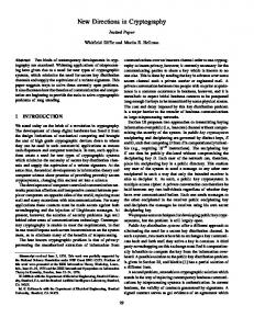
Figure 1. Anomaly Detection Architecture. The sensor measurements yk and the control commands uk are fed to the anomaly detection block. Under normal operating conditions, the actuation on the plant corresponds to the intended action by the controller: vk = uk , and the observations are correctly reported back to the controller: yk = zk .

Actuators

uk

vk 6= uk


zk

yk


uk

Reconfi guration

rk

Sensors

Controller

Detection

Figure 2. When one or more actuation signals are compromised (e.g., the actuator itself is compromised or it receives and accepts a control command from an untrusted entity) the actuation to the plant will be different to the intended action by the controller: vk ≠ uk . This false actuation will in turn affect the measured variables of the plant zk which in turn affect the sensor measurements reported back to the controller: yk = zk .

deceive the controller about the real state of the plant. In the worst case, the control device can be compromised as well, giving the attacker potentially unlimited control on the plant to implement any outcome (see Fig. 4). This last figure also captures the threat model from a malicious control command sent from the control center as seen in Fig. 5: While the implementation might be different–one monitor is placed in the supervisory network and the other monitor on the field communications interface–the logical architecture–what the monitoring application sees–will be the same. In these attack schemes we assume that the control has a trusted detection mechanism, which can recognize unexpected behaviors and potentially take counter measures. The detection block in Figs. 1- 4 is expanded in Fig. 6 to illustrate several alternative algorithms we found in the literature. There are two blocks that are straightforward to implement: (1) The controller block in Fig. 6 is a redundant control algorithm (i.e., in addition to the controller of Fig. 1) that checks if the controller is sending the appropriate uk to the field, and (2) The safety check block is an algorithm that checks if the predicted future state of the system will violate a safety specification (e.g., the pressure in a tank will exceed its safety limit). The different alternative detection algorithms are also summarized in Table I. In this paper, we focus on analyzing the more challenging algorithms: 1) Prediction (Physical Model): given sensor yk and control commands uk , a model of the physical system will predict a future expected measurement yˆk+1 . 2) Anomaly detection (Statistical Test): Given a time series of residuals rk (the difference between the received sensor measurement yk and the predicted/expected measurement yˆk ), the anomaly detection test needs to determine when to raise an alarm. By focusing on these algorithms our detection block can be simplified as shown in Fig. 7.

3


vk

Actuators

uk


zk

yk 6= zk


uk

Reconfi guration

rk

Sensors

Controller

Detection

Figure 3. When one or more sensor signals are compromised (e.g., the sensor itself is compromised or the controller receives and accepts a sensor measurement from an untrusted entity) the sensor measurement used as an input to the control algorithm will be different from the real state of the measured variables yk ≠ zk .

vk

Actuators


zk

Sensors

uk 6= K(yk )

yk

(without reconfiguration)

Reconfi guration

rk

uk 6= K(yk )

Controller

Detection

Figure 4. When the controller is compromised, it will generate a control signal that does not satisfy the logic of the correct control algorithm: uk ≠ K(yk ).

B. Taxonomy We now present our new taxonomy for related work, based on four aspects: (1) model for physical system, (2) trust model, (3) detection mechanism proposed, and (4) evaluation metrics. 1) Physical System Model: LDS or AR: The model of how a physical system behaves can be developed from physical equations (Newton’s laws, fluid dynamics, or electromagnetic laws) or it can be learned from observations through a technique called system identification [6], [58]. In system identification one often has to use either Auto-Regressive Moving Average with eXogenous inputs (ARMAX) or linear state-space models. Two popular models used by the papers we survey are AutoRegressive (AR) models (e.g., used by Hadziosmanovic et al. [30]) and Linear Dynamical State-Space (LDS) models (e.g., used by PyCRA [84]). AR models are a subset of ARMAX models but without modeling external inputs or the average error

Control Center

y

Supervisory Control Network

y

Figure 5. Attacks on Central Control or Supervisory Control Network translate on the logical model shown in Fig. 4.

4


Figure 6. The detection block from Fig. 1, with a set of different detection algorithms. In the top, the controller block is a redundant control (i.e., in addition to the controller of Fig. 1) that checks if the control commands are appropriate. The middle row (prediction, residual generation, and anomaly detection blocks) focuses on looking at the sensor values and raising an alarm if they are different to what we expect/predict. The prediction and safety check blocks focus on predicting the future state of the system, and if it violates a safety limit then we raise an alert.

Detection Residual Generation

yk yk uk

1

Physical Model LDS or AR

yˆk

rk = yk

yˆk

rk

Anomaly Detection: Sateless or Stateful

alert

Figure 7. The detection module from Fig. 6 focusing on using anomaly detection based on the physics of the process.

and LDS are a subset of state space models. If we only have output data (sensor measurements yk ), regression models like AR, ARMA, or ARIMA are a popular way to learn the correlation between observations. Using these models we can predict the next outcome. For example, for an Auto-Regressive (AR) model, the prediction would be k

yˆk+1 = ∑ αi yi + α0

(1)

i=k−N

where αi are the coefficients learned through system identification and yi the last N sensor measurements—where the amount of parameters to learn N can be also estimated to prevent over-fitting of the model using tools like Akaike’s Information Criteria (AIC). It is possible to obtain the coefficients αi , by solving an optimization problem that minimizes the residuals (e.g., least squares) [56]. If we have inputs (control commands uk ) and outputs (sensor measurements yk ) available, we can use subspace model identification methods, producing the following model: xk+1 = Axk + Buk + Ek yk = Cxk + Duk + ek

(2)

Table I

D ETECTION A LGORITHM A LTERNATIVES FOUND IN L ITERATURE

Features Cur. In & Prev. Out Prev. Sensor Observ.

uk , yk−1 yk−1 , yk−2 , . . . , yk−N

Prediction Input-Output LDS Output-Only AR

xk+1 = Axk + Buk v + Ek yk = Cxk + Duk + ek k yk+1 = ∑i=k−N αi yi + α0 + Ek

Anomaly Detection ?

Stateless

∣rk ∣ > τ

Stateful

S0 = 0. (Sk + ∣rk ∣ − δ) > τ

+ ?

5

C. State Estimation Control Logic

uk = K x ˆk x ˆk uk yk

Prediction

1 1

State Estimation

x ˆk

yˆk = C x ˆk

Bad Data Detection

||yk

Cx ˆk || > ⌧

}


where A, B, C, and D are matrices modeling the dynamics of the physical system. Most physical systems are strictly causal p n and then therefore usually D = 0. The control commands uk ∈ R affect the next time step of the state of the system xk ∈ R q and sensor measurements yk ∈ R are modeled as a linear combination of these hidden states. ek and Ek are sensor and perturbation noise, and are assumed to be a random process with zero mean. To make a prediction, we i) first need yk and uk to obtain a state estimate x ˆk+1 and ii) use the estimate to predict yˆk+1 = Cx ˆk+1 (if D is not zero we also need uk+1 ). Some communities adopt models that employ the observation equation from (2) without the dynamic state equation. We refer to this special case of LDS as Static Linear State-space (SLS) model. 2) Trust Model: To evaluate attack detection schemes, it is important to explicitly state which components in the control loop (or complete system) need to be trusted in order to correctly detect attacks. We call such explicit assumptions a trust model, and summarize such explicit or implicit assumptions for the related work. The trust model is related to attacker models, that often explicitly specify which components can be compromised (or not). Devices that cannot be compromised are trustworthy, so both model views are certainly related. The attacker model is more focused on the attacker, and the trust model more focused on the system under attack. We discuss trust assumptions in § VI. 3) Detection Mechanism: Stateless or Stateful: Based on the observed sensor or control signals up to time k, we can use models of the physical system (e.g., AR or LDS) to predict the expected observations yˆk+1 (note that yˆk+1 can be a vector representing multiple sensors at time k + 1). The difference rk between the observations predicted by our model yˆk+1 and the sensor measurements received from the field yk+1 is usually called a residual. If the observations we get from the sensors yk are significantly different from the ones we expect (i.e., if the residual is large), we can generate an alert. In a Stateless test, we raise an alarm for every single significant deviation at time k: i.e., if ∣yk − yˆk ∣ = rk ≥ τ , where τ is a threshold. In a Stateful test we compute an additional statistic Sk that keeps track of the historical changes of rk (no matter how small) and generate an alert if Sk ≥ τ , i.e., if there is a persistent deviation across multiple time-steps. There are many tests that can keep track of the historical behavior of the residual rk such as taking an average over a time-window, an exponential weighted moving average (EWMA), or using change detection statistics such as the non-parametric CUmulative SUM (CUSUM) statistic. The theory behind CUSUM assumes we have a probability model for our observations rk (the residuals in our case); this obscures the intuition behind CUSUM, so we focus on the non-parametric CUSUM (CUSUM without probability likelihood models) which is basically a sum of the residuals. In this case, the CUSUM statistic is defined recursively as S0 = 0 and + + Sk+1 = (Sk + ∣rk ∣ − δ) , where (x) represents max(0, x) and δ is selected so that the expected value of ∣rk ∣ − δ < 0 under hypothesis H0 (i.e., δ prevents Sk from increasing consistently under normal operation). An alert is generated whenever the statistic is greater than a previously defined threshold Sk > τ and the test is restarted with Sk+1 = 0. 4) Evaluation Metric: The evaluation metric is used to determine the efficacy of the proposed detection scheme. Ideally, the metric should allow for a fair comparison of different schemes that are targeting the same adversarial model for comparable settings. Common evaluation metrics are the number of false alerts, and the probability of detecting attacks. A parametric curve illustrating the trade-off of these two quantities is the Receiver Operating Characteristic (ROC) curve. A specific combination of these two metrics into a single quantity is the accuracy (correct classification) of the anomaly detector.

Residual

rk

x ˆk Safety Check

x ˆk 2 Allowed States? Figure 8. Whenever the sensor measurements yk do not observe all the variables of interest from the physical process, we can use state estimation to obtain an estimate x ˆk of the real state of the system xk at time k (if we have a model of the system). State estimates can then be used for the control logic, for prediction (and therefore for bad data detection), and for safety checks.

Before we start our survey we also need some preliminaries in what state estimation is. Whenever the sensor measurements ˆk yk do not observe all the variables of interest from the physical process, we can use state estimation to obtain an estimate x of the real state of the system xk at time k (if we have a model of the system).

6


Recall Eq. (2) gives us the relationship between the observed sensor measurements yk and the hidden state xk . The naive −1 approach would assume the noise ek is zero and then solve for xk : xk = C (yk − Duk ); however, for most practical cases this is not possible as the matrix C is not invertible, and we need to account for the variance of the noise. The exact solution for this case goes beyond the scope of this paper, but readers interested in finding out how to estimate the state of a dynamical system are encouraged to read about Luenberger observers [88] and the Kalman filter [98], which are used to dynamically estimate the system’s states without or with noise, respectively. State estimates can then be used for the control logic, for prediction (and therefore for bad data detection), and for safety checks, as in Fig. 8. Outside of the literature for state estimation in the power grid [55], there has been little work in studying the role of state estimation for the security of other cyber-physical systems. Towards the end of this paper we illustrate the use of state estimation for an industrial control system of four water tanks, and we show how state estimation is useful for tracking variables which are not observed by the sensor measurements. This example will show again the importance of considering the input uk as part of the anomaly detection model. IV. S URVEY OF W ORK ON P HYSICS - BASED ATTACK D ETECTION IN C ONTROL S YSTEMS

In this section, we survey previous work and relate it to the general framework we have introduced.

A. Power Systems Attacks on bad data detection. One of the most popular lines of work within the scope of our paper is the study of false-data injection attacks to avoid being detected by bad data detection algorithms for state estimation in the power grid. In the power grid, operators need to estimate the phase angles xk from the measured power flow yk in the transmission grid. These bad data detection algorithms were meant to detect random sensor faults, not strategic attacks, and as Liu et al. [54], [55] showed, it is possible for an attacker to create false sensor signals that will not raise an alarm (experimental validation in software used by the energy sector was later confirmed [92]). Model of the Physical System: It is known that the measured power flow yk = h(xk ) + ek is a nonlinear noisy measurement of the state of the system x and an unknown quantity ek called the measurement error. Liu et al. considered the linear model where yk = Cxk + ek , therefore this model of the physical system is the sensor measurement SLS model described by Eq. (2), where the matrix D is zero and without the dynamic state equation. ˆk , the state Detection: the mechanism they consider is a stateless anomaly detection test, where the residual is rk = yk − Cx T −1 −1 T −1 estimate is defined as x ˆk = (C W C) C W yk and W is the covariance matrix of the measurement noise ek . Note that because rk is a vector, the metric ∣ ⋅ ∣ is a vector distance metric, rather than the absolute value. This test is also illustrated in the middle row of Fig. 8. Trust Model: The sensor data is manipulated, and cannot be trusted. The goal of the attacker is to create false sensor measurements such that ∣rk ∣ < τ . Evaluation Metrics: The paper focuses on how hard it is for the adversary to find attacks such that ∣rk ∣ < τ . There has been a significant amount of follow up research focusing on false data injection for state estimation in the power grid, including the work of Dán and Sandberg [20], who study the problem of identifying the best k sensors to protect in order to minimize the impact of attacks (they assume the attacker cannot compromise these sensors). Kosut et. al. [45] consider attackers trying to minimize the error introduced in the estimate, and defenders with a new detection algorithm that attempts to detect false data injection attacks. Liang et al. [51] consider the nonlinear observation model yk = h(xk ) + ek . Further work includes [11], [28], [42], [76], [81], [91], [96]. Automatic Generation Control. Control centers in the power grid send Area Control Error (ACE) signals to ramp up or ramp down generation based on the state of the grid. Sridhar and Govindarasu [89] consider an ACE signal that cannot be trusted. Model of the Physical System: A historical model of how real-time load forecast affects ACE. Detection: The ACE computed by the control center (ACER ) and the one computed from the forecast (ACEF ) are then compared to compute the residual. They add the residuals for a time window and then raise an alarm if it exceeds a threshold. Trust Model: The load forecast is trusted but the ACE signal is not. Evaluation Metric: False positive and false negative (1-detection) rates. Active monitoring. While most of the papers we consider in this survey use passive monitoring (they do not interfere with normal operation unless there is an alarm and a reconfiguration is triggered), the works of Morrow et al. [70] and Davis et al. [21] consider active monitoring, that is, they use the optional reconfiguration signal we defined in Fig. 1 to change the system periodically, even if there are no indicators of attacks. The intuition behind this approach is to increase the effort of an adversary that wants to remain undetected, because this reconfiguration will change the state of the system and if the adversary does not change its sensor false data injection attack appropriately, then it might be detected by an anomaly detection that will look for the intended change in the sensor values. The idea of active monitoring has also been proposed in other domains [68], [84], [95]. While the idea of perturbing the system to reveal attackers that don’t adapt to these perturbations is intuitively appealing, it also comes with an operational cost: the deviation of a system from an ideal operational state just to test if the sensors have

7


been compromised or not might not sound very appealing to control engineers and asset owners whose livelihood depends on the optimal operation of a system. However, there is another way to look at this idea: if the control signal uk is already highly variable (e.g., in the control of frequency generators in the power grid who need to react to constant changes in the power demand of consumers), then the system might already be intrinsically better suited to detect attacks via passive monitoring. We will explore this idea in § VIII. B. Industrial Control Systems Real-world Modbus-based Detection. Hadziosmanovic et al. [30] give us a good example of how to use Modbus (an industrial protocol) traces from a real-world operational system to detect attacks by monitoring the state variables of the system, including: constants, attribute data, and continuous data. We focus on their analysis of continuous data because this research is a motivation for our own experiments in this paper. Model of the Physical System: To model the behavior of continuous sensor observations yk like the water level in a tank or the water pressure in a pipe, the authors use an AR model as we described in Eq. (1). This corresponds to models of individual signals, and as we will show in our experiments, if we can create models that show the correlation of multiple variables we can obtain better attack detection algorithms. In fact, that was an observation made by the authors, as they found that multiple variables exhibit similar (even identical) behavior. Detection: The scheme raises an alert if (1) the measurement yk reaches outside of specified limits (this is equivalent to the Safety Check box in Fig. 6) or (2) yk produces a deviation in the prediction yˆk of the autoregressive model (noting that rk = yk − yˆk ), this is the stateless statistical test from Fig. 6. Trust Model: It is not clear where in the control architecture the real-world data trace was collected. Because deploying a large-scale collection of a variety of devices in a control network is easier at the supervisory control network, it is likely that the real-world traffic monitors data exchanged between the control centers and the PLCs. In this case the PLC must be trusted, and therefore the adversary must attack the actuators or the sensors. Evaluation Metrics: The paper focuses on understanding how accurately their AR system models the real-world system and identifying the cases where it fails. They mention that they are more interested in understanding the model fidelity rather than in specific true/false alarm rates, and we agree with them because measuring the true positive rate would be an artificial metric. Understanding the model fidelity is implicitly looking at the potential of false alarms because deviations between predictions and observations during normal operations are indicators of false alarms. While this is a good approach for the exploratory data analysis done in the paper, it might be misunderstood by future proposals. After all, the rule never raise an alert will have zero false alarms (but it will never detect any attack). We discuss this further in § V. Attack Localization. State Relation-based Intrusion Detection (SRID) [97] attempts to detect attacks, and then find the root cause of the attack in an industrial control system. SRID is an outlier in our survey, despite a growing literature that follow similar approaches for the topic of using the physics of CPS to detect attacks, SRID proposes system identification, and bad data detection tests that are unique. Model of Physical System: Instead of using a traditional and well-understood system identification approach to learn a model of the boiler simulator they study, they propose a set of heuristics they name feedback correlations and forward correlations; however, we were not able to find a good justification as to why these heuristics are needed, or why they are better than traditional system identification methods. We recommend that for any future work, if the authors propose a new system identification tool (previously untested), they should use a traditional tool to test as a baseline approach. One of the goals of SRID is to identify the location of an attack; but we believe that if we know all the control loops in their boiler simulation, we can create models for each of them and identify the root cause using traditional methods; however, the paper does not mention where other researchers can find the boiler simulator SRID used in the experiments, so we cannot compare our methods to theirs. Detection: SRID does not specify if they use control and sensor measurements for their anomaly detection, but from the description it appears they use only sensor measurements. SRID proposes a new bad data detection based on alternation vectors, which basically tracks the history of measured variables going up or down. If this time series is not an allowable trend (not previously seen) the detection test generates an alert. It is not clear why this heuristic can perform better than the traditional residual generation approach. Trust Model: The sensors cannot be trusted, but the attacker sends arbitrary data that falls within the sensor’s valid range. Therefore, this attacker is not strategic and it behaves exactly as random faults. It is not clear therefore how their evaluation will differ whenever there is a sensor fault (within the valid range) or the attacker they propose. Evaluation Metrics: SRID measures the successful attack detection rate and the false alarm rate. Attack-Detection and Response. Cardenas et al. [14] consider a chemical industrial control system. Model of the Physical System: The authors approximate the nonlinear dynamics of the chemical system with an input/output linear system, as we defined in Eq. (2). Therefore this model captures the correlations among multiple different observations yk (with the matrix C) but also the correlation between input uk and output yk and is therefore a model that can match the fidelity of observations very closely. Detection: The authors use the linear system to predict yˆk given the previous input uk−1 and the previous measurement yk−1 and then test whether or not the prediction is close to the observed measurement rk = yk − yˆk . They raise an alert if the CUSUM statistic (the stateful test of Fig. 6) is higher than a threshold. Trust Model: One or more sensors are compromised, and cannot be trusted. The goal of the adversary is to violate the safety of the system: i.e., an attacker that wants to raise the

8


pressure level in the tank above 3000kPa and at the same time remain undetected by the test. The actuators and the control logic are assumed to be trusted. Evaluation Metrics: The paper proposes a control reconfiguration whenever an attack is detected, in particular a switch to open-loop control, meaning that the control algorithm will ignore sensor measurements and will attempt to estimate the state of the system based only on the expected consequences of its own control commands. As a result, instead of measuring the false alarm rate, the authors measure the impact of a reconfiguration triggered by a false alarm on the safety of the system—in other words, a false alarm must never drive the system to an unsafe state (a pressure inside the tank greater than 3000kPa). To evaluate the security of the detection algorithm, the authors also test to see if an attacker that wants to remain undetected can drive the pressure inside the tank above 3000kPa. Clustering. Another approach to detect attacks in process control systems is to learn unsupervised clustering models containing the pair-wise relationship between variables of a process, and then identify potential attacks as anomalies that do not fit these clusters [43], [47]. These approaches are non-parametric, which have the advantage of creating models of the physical process without a priori knowledge of the physics of the process; however, a non-parametric approach does not have the fidelity to the real physics of the system as an LDS or AR model will have, in particular when modeling the time-evolution of the system or the evolution outside of a steady state. Detecting Safety Violations and Response. Another paper that proposes control reconfiguration is McLaughlin [61]. This paper tackles the problem of how to verify that control signals uk will not drive the system to an unsafe state, and if they do, to modify the control signal and produce a reconfiguration control that will prevent the system from reaching an unsafe state. As such this is one of the few papers that considers a reconfiguration option when an attack (or possible safety violation) is 2 detected. The proposed approach, C , mediates all control signals uk sent by operators and embedded controllers to the physical 2 system. System Model: C considers multiple systems with discrete states and formal specifications, as such this approach is better suited for systems where safety is specified as logical control actions instead of systems with continuous states (where we would need to use system identification to learn their dynamics). Detection: This approach is most similar to the attack on control signals in Fig. 2. However, their focus is not to detect if uk ≠ K(yk ), but to check if uk will violate a safety condition of the control signal or not. As such, their approach is most similar to using the Safety Check block we introduced in Fig. 6. Trust Model: McLaughlin mentions that “the approach can prevent any unsafe device behavior caused by a false data injection 2 attack, but it cannot detect forged sensor data” and later in the paper we find “C mitigates all control channel attacks against devices, and only requires trust in process engineers and physical sensors.” This is a contradiction, and the correct statement to 2 satisfy the security of their model is the latter. As such C assumes trusted sensors and trusted actuation devices (specifically 2 stating trusted actuators is a missing trust assumption in their model). C is related to traditional safety systems for control like safety interlocks, and not necessarily malicious attacks as there does not seem to be a difference between preventing an unsafe 2 accidental action to an unsafe malicious action. Evaluation Metrics: There are three main properties that C attempts to hold: 1) safety (the approach must not introduce new unsafe behaviors, i.e., when operations are denied the ‘automated’ control over the plant should not lead the plant to an unsafe state), 2) security (mediation guarantees should hold under all attacks allowed by the threat model), and 3) performance (control systems must meet real time deadlines while imposing minimal overhead). Detecting malicious control commands. There is other related work in trying to understand consequences of potentially malicious control commands from the control center, and as such they correspond (logically) to the attack on control signals in Fig. 2 [46], [53], [72]. Their goal is to understand safe sequences of commands, and commands that might create problems to the system. For example, Lin et al. [53] considers contingency analyses to predict consequences of control commands and Mitra et al. [66] combine the dynamics of the system with discrete transitions (finite state machines) such as interruptions. Using set theory, they show it is possible to determine the set of safe states, the set of reachable states, and invariant sets; therefore, if there is not an input that can drive the states out of the safety set, the model is safe. Finding these sets requires some relaxations and a good knowledge of the behavior and limitations of the system. 2

Critical State Analysis. Carcano et al. [13] propose a safety monitoring system similar to C but without mediating control commands (and using the control command uk to predict the next state yˆk to see if it violates a safety condition) or proposing any reconfiguration when a safety issue is detected. The proposed concept is to monitor the state of a system and raise alerts whenever it is in a critical state (or approaching a critical state). Model of the Physical System: the approach measures the c c distance of sensor measurements yk to a critical state y : d(yk , y ). They do not learn the dynamics of the physical system and this can have serious consequences as for example the power grid can change the distance to a critical state almost immediately whereas chemical processes such as growing bacteria in anaerobic reactors can take days to drive a system state to an unsafe region. Detection: They raise an alert whenever the system is in a critical state and also log the packets that led the system to that state for forensic purposes. They only monitor yk not uk , which as we will show, is a suboptimal approach. Trust Model: Because the authors monitor Modbus commands, it is likely that their sniffer is installed at the Supervisory Control Network of Fig. 9, and as we will show, this assumes a trusted PLC. They also assume trusted sensors. The simulated attacks consist of legitimate control commands that drive the system to unsafe states; as such, these attacks are easy to detect. Evaluation Metrics: they monitor the number of false alarms and the true positive rate. The detection algorithm can have missed positives

9


(when an attack happened and was not detected) because of packet drops but it is not clear what a false alarm is in their case (it appears to be a critical state caused by legitimate control actions). C. Control Theory There is a significant body of work in attack detection from the control theory community [8], [9], [34], [48], [64]. While the treatment of the topic is highly mathematical (a recent special issue of the IEEE Control Systems Magazine provides an accessible introduction to the topic [35]), we attempt to extract the intuition behind key approaches to see if they can be useful for the computer security community. Most control papers we reviewed look at models of the physical system satisfying Eq. (2) because that model has proven to be very powerful for most practical purposes. In addition, most of the control theory papers we reviewed assumed a stateless detection. We think this bias towards the stateless test by the control theory community stems from the fact that the stateless test allows researchers to prove theorems and derive clean mathematical results. In contrast, providing such thorough theoretical analysis for stateful tests (e.g., CUSUM) can become intractable for realistic systems. We believe that this focus on strong analytical results prevents the use of stateful tests that effectively perform better in many practical cases. In § VIII, we compare stateful and stateless tests, and show that the CUSUM stateful tests clearly outperform stateless statistics in many practical cases. Zero-dynamics attacks. These attacks are interesting because they show that even without compromising sensors, attackers can mislead control systems into thinking they are at a different state. The attacks require the attacker to compromise the actuators, that the anomaly detection system monitors the legitimate control signal uk and the legitimate sensor signal yk , and a plant vulnerable to these attacks. One of the fundamental properties control engineers ask about Eq. (2) is whether or not the system is Observable [88]. If it is observable, then we know that we can obtain a good state estimate x ˆk given the history of previous control inputs uk and sensor measurements yk . Most practical systems are observable or are designed to be observable. Now, if we assume an observable system, then we can hypothesize that the only way to fool a system into thinking it is at a false state, is by compromising the sensors and sending false sensor readings. Zero-dynamics attacks are an example that this hypothesis is false [73], [93], [94]. Zero-dynamics attacks require attackers that compromise actuation signals as shown in Fig. 2: that is, the anomaly detector observes a valid uk and a valid yk , but it does not observe the compromised vk . Not all systems are vulnerable to these attacks, but certain systems like the quadruple tank process [39] can be (depending on the specific parameters). Though zero-dynamics attacks are interesting from a theoretical point of view, most practical systems will not be vulnerable to these attacks (although it is always good to check these conditions). First, if the sensors monitor all variables of interest, we won’t need state estimation (although this might not be possible in a large-scale control system with thousands of states); second, even if the system is vulnerable to zero-dynamics attacks, the attacker has to follow a specific control action from which it cannot deviate (so the attacker will have problems achieving a particular goal—e.g., move the system to a particular state), and finally, if the system is minimum phase, the attacker might not be able to destabilize the system. In addition, there are several recommendations on how to design a control system to prevent zero-dynamic attacks [94]. Combined use of cyber- and physical attacks. Control theory papers have also considered the interplay between physical attacks and cyber-attacks. In a set of papers by Amin et al. [3], [4] the attacker launches physical attacks to the system (physically stealing water from water distribution systems) while at the same time it launches a cyber-attack (compromised sensors send false data masking the effects of the physical attack). We did not consider physical attacks originally, but we then realized that the actuation attacks of Fig. 2 account for physical attack, as it is equivalent to the attacker inserting its own actuators, and therefore the real actuation signal vk will be different from the intended control command uk . To detect these attacks, they propose the use of unknown input observers; however, the bottom line is that if the attackers control enough actuation and sensor measurements, there is nothing the detector can do as the compromised sensors can always send false data to make the detector believe the system is in the state the control wanted it to go. These covert attacks have been characterized for linear [86] and nonlinear systems [87]. Active Monitoring. The idea of reconfiguring the control system by sending unpredictable control commands and then verifying that the sensor responds as expected is referred to here as active monitoring (see § IV-A). The work of Mo et al. [67]–[69] considers embedding a watermark in the control signal. This is useful for systems that remain constant for long periods of time (if they are in a steady state) and by randomly perturbing the system, an analyst can see if the sensor values respond appropriately, although an attacker that knows the dynamics of the system and the control commands can craft an appropriate false sensor response that will not be detected by the security analyst. Energy-based attack detection. Finally, another detection mechanism using control theoretic components was proposed by Eyisi and Koutsoukos [23]. The main idea is that the energy properties of a physical system can be used to detect errors or attacks. Unlike observer-based detection (used by the majority of control papers), their work uses concepts of energy or

10


passivity, which is a property of systems which consume but not produce net energy. In other words, the system is passive if it dissipates more energy than it generates. To use this idea for detecting attacks, the monitor function estimates the supplied energy (by control commands) and compares it to the energy dissipated and the energy stored in the system (which depend on the dynamics of the system). While the idea is novel and unique, it is not clear why this approach might be better than traditional residual-based approaches, in particular given that any attack impersonating a passive device would be undetected, and in addition, the designer needs more information. To construct an energy model, a designer needs access to inputs and outputs, the model of the system in state space (as in Eq. (2)), and functions that describe the energy dissipation of a system in function of the stored energy (energy function) and the power supply (supply function). D. Miscellaneous Domains There is a growing interest in using the physics of other control systems to detect attacks in a variety of domains. Active Monitoring for Sensors. Active monitoring has also been used to verify the freshness and authenticity of a variety of sensors [84] and video cameras [95]. PyCRA [84] uses an LDS model to predict the response of sensors and to compute the 2 residual rk , which is then passed to a stateful χ anomaly detection statistic. The attacker in PyCRA has a physical actuator to respond to the active challenge. The evaluation of the proposal focuses on computing the trade-off between false alarms and probability of detection (i.e., ROC curves). Another active monitoring approach suggests visual challenges [95] in order to detect attacks against video cameras. In particular a trusted verifier sends a visual challenge such as a passphrase or Quick Response (QR) code to a display that is part of the visual field of the camera, and if the visual challenge is detected in the video relayed by the camera, the footage is deemed trustworthy. The paper considers an adversary model that knows all the details of the system and tries to forge video footage after capturing the visual challenge. The authors use the CUSUM statistic to keep track of decoding errors. Automated Vehicles. Kerns et al. [41] consider how Global Positioning System (GPS) spoofing attacks can take control over unmanned aircrafts. They use an LDS as a model of the physical system, and then use a stateless residual (also referred to as innovations) test to detect attacks. They show two attacks, one where the attacker is detected, and another one where the attacker manages to keep all the residuals below the threshold while still changing the position of the aircraft. Sajjad et al. [79] consider the control of cars in automated platoons. They use LDS to model the physical system and then use a stateful test with a fixed window of time to process the residuals. To evaluate their system they show that when attacks are detected, the cars in the platoon can take evasive maneuvers to avoid collisions. Physics-based forensics. Conotter et al. [18] propose to look at the geometry and physics of free-falling projectiles to check if the motions of a moving object in videos are realistic or fake. The proposed algorithm to detect implausible trajectories of objects follows: First, describe a simplified 3D physical model of the expected trajectory and a simplified 2D imaging model. Then, determine if the image of the trajectory of a projectile motion is consistent with the physical model. A contribution of the paper is to show how a 3D model can be directly created from the 2D video footage. Once a 3D model is created, it can be used to check against the physical model to detect any deviations. The attacker is someone who uses sophisticated video editing tools to manipulate a video of for example, a person throwing a basketball to create a perfect, spectacular shot. In this case, the forger has access to the 2D video footage and can manipulate, re-process it. The paper does not focus on how the forgery is done, but assumes that a video can be either fake or real, and the goal of the proposed approach is to determine the authenticity of each video. However, note that only naive attackers were considered here. If the forger is aware of such detection mechanism, it will try to manipulate the 2D image to conform to the real 3D model. The evaluation metric computes the mean error between the pair of representations of the projectile motion using Euclidean distance; so it is a stateful test. The reason for using this test (and not change detection statistics) stems from the fact that forgery detection does not need to be done in real-time, but it is mostly done after the fact. Electricity theft. There is also work on the problem of electricity theft detection by monitoring real traces from electricity consumption from deployed smart meters [59]. To model the electricity consumption the authors use ARMA models, which are output-only models similar to those in Eq. (1). Since their detection is not done online (similar to the video forensics case), the detection test is not stateless but stateful (an average of the residuals), where the detector can collect a lot of data and is not in a rush to make a quick decision. The attacker has compromised one sensor (the smart meter at their home) and sends false electricity consumption. The evaluation metric is the largest amount of electricity that the attacker can steal without being detected. Medical devices. Detection of attacks to medical devices is also a growing interest [31], [32]. Hei et al. [31] study overdose attacks/accidents for insulin pumps and employ a supervised learning approach to learn normal patient infusion patterns with dosage amount, rate, and time of infusion. The model of their physical system is done through a Support Vector Regression (SVR). Again, similar to all the papers reviewed in this miscellaneous section focusing on off-line anomaly detection, the detection test is an average of the residuals. More specifically, they use the Mean Squared Error measuring the difference between the predicted and the real value before raising an alert.

11

[11] Bobba et al. [81] Sandberg et al. [91] Teixeira et al. [8] Bai, Gupta [67] Mo et al. [68] Mo, Sinopoli [9] Bai et al. [64] Miao et al. [34] Hou et al. [23] Eyisi et al. [69] Mo et al. [73] Pasqualetti et al. [94] Teixeira et al. [48] Kwon et al. [93] Teixeira et al. [22] Do et al. [3], [4] Amin et al. [86] Smith [41] Kerns et al. [51] Liang et al. [28] Giani et al. [20] Dan, Sandberg [45] Kosut et al. [42] Kim, Poor [21] Davis et al. [89] Sridhar, Govindarasu [46] Koutsandria et al. [59] Mashima et al. [54], [55] Liu et al. [72] Parvania et al. [53] Lin et al. [84] Shoukry et al. [30] Hadziosmanovic et al. [14] Cardenas et al. [97] Wang et al. [61] McLaughlin [80] Sajjad et al. [95] Valente, Cardenas [47] Krotofil et al. [96] Vukovic, Dan [70] Morrow et al. [19] Cui et al. [13] Carcano et al. [31] Hei et al. [43] Kiss et al.


Table II

S UMMARY OF TAXONOMY OF RELATED WORK ON PHYSICS - BASED ATTACK DETECTION IN CONTROL SYSTEMS .

Venue

Control

Smart/Power Grid

Security

Misc.

Detection stateless ● ● ● - - - ● ● ● ) ( ● ● ● ● ● - ● ( ) ● - ● ● ● ● ● - ● - ● ) ( ● - ● - ( ) ) ( - - ● ● ● ● ● - ● stateful - - - ( ) ⊛ ⊛ - - - - - - - - - ● - - - ⊛ - - - - - ⊛ - ● - - - ⊛ - ● - - ● ● ● - - ● - ⊛ Model AR - - SLS ● ● ( ) LDS - - other - - -

● -

● -

● -

● -

● -

● -

● -

● -

● -

● -

● -

● -

● -

● -

● -

● -

● -

● -

● -

● -

● -

( ) -

●

●

● -

● -

( )

- - - ● ) ( -

● -

● -

●

●

● -

●

●

) ( -

( ) -

● -

●

( )

●

● -

● ● ●

● -

● -

● -

● ● -

● -

● ●

● ● -

● ● -

● ● -

● ● -

● ●

● -

-

● -

● ● -

● -

● -

● ● ●

● -

-

● ●

● ● -

● ●

● ● -

-

● -

● ●

● -

-

● ●

-

● -

● -

● -

● ● -

-

● ● -

● ●

● -

●

∗

Metrics impact statistic TPR FPR

-

● -

● -

Not Trusted ‡ † sensors ● ● ● ● ● ● - ● ● ● ● ● ● ● ● ● ● ● ● ● ● ● ● ● ● - - ● ● - - ● ● ● ( ) - - ● ● - ● ● actuators - - - - ● ● ● - - - ● ● ● ● ● ● - ● - - - - - - - - - - - ● - - ( ) - - - - - - - - controllers - - - - - - - - - - - - - - - - - - - - - - - - - ● - - - - ● - - - - ● ● - - ● - Validation simulation real data testbed

† ( ) - ● - ● ) - (

- ● ● ● ● ● ● ● ● ● ● ● ● ● - ● - ● ● ● - ● ● ● ● ● ) ( - ● - ● - - ● ● - ● - ● ● ● ● - - ● - - - - - - - - - - - - - - - - ● - - - - - - - ) ( ● - ● - - - - ● - - - - ● - - - - - ● - - - - - - - - - - - - - - ● - - - ● - - - - - - - - - - ( ) - ● ● - - ● - - - - - - ● -

Monitoring ◇ ◇ ◇ ◇ ◇ ◇ ◇ ◇ ◇ ◇ ◆ ◇ ◇ ◇ ◇ ◇ ◇ ◇ ◇ ◇ ◇ ◇ ◇ ◇ ◆ ◇ ◇ ◇ ◇ ◇ ◇ ◆ ◇ ◇ ◇ ◇ ◇ ◆ ◇ ◇ ◆ ◇ ◇ ◇ ◇ Legend: ●: feature considered by authors, ( ): feature not explicitly stated or exhibits ambiguity, ⊛: a windowed stateful detection method is used, ◇: ∗ passive monitoring, ◆: active monitoring, †: attacks are made on the communication layer, ‡: also considers physical attacks, Evaluation options have been abbreviated in the table: Attack Impact, Statistic Visualization, True Positive Rate, False Positive Rate.

V. D ISCUSSION AND S UGGESTIONS We apply our taxonomy to previous work in Table II. We arrange papers by conference venue (we assigned workshops to the venue that the main conference is associated with). We also assigned conferences associated with Cyber-Physical Systems Week (CPSWeek) to control conferences because of the overlap of attendees to both venues. We make the following observations: (1) the vast majority of prior work uses stateless tests; (2) most control and power grid venues use LDS (or their static counterpart SLS) to model the physical system, while computer security venues tend to use a variety of models; several of them are non-standard and difficult to replicate by other researchers; (3) there is no consistent metric used to evaluate proposed attack-detection algorithms; (4) most papers focus on describing attacks to specific devices (i.e., devices that are not trusted) but they do not provide a fine-grain trust model that can be used to described what can be detected and what cannot be detected when the adversary is in control of different devices; and (5) no previous work has validated their work with all three options: simulations, testbeds, and real-world data. A. General shortcomings 1) No Consistent Evaluation. There is no common evaluation metric used across multiple papers. Some papers [13], [97] measure the accuracy of their anomaly detector by looking at the trade-off between the false alarm rate and the true positive rate (metrics that are commonly used in machine-learning, fault-detection, and some intrusion detection papers), while others [30] argue that measuring the true positive rate is misleading in a field that has not enough attack samples, so they focus only on measuring the fidelity of their models (i.e., minimizing the false alarms). In addition, most papers focusing

12

3) Lack of Trust Models. Most papers do not describe their trust models with enough precision. Information exchanged between field devices (sensor to controller and controller to actuator in Fig. 1) is communicated through a different channel from information that is exchanged between controllers or between controller and the supervisory control center. Papers that monitor network packets in the supervisory control network [30] implicitly assume that the controller (PLC) they monitor is trusted, otherwise the PLC could fabricate false packets that the monitor expects to see, while at the same time sending malicious data to actuators (what Stuxnet did). Thus, we need to monitor the communication between field devices in order to identify compromised PLCs in addition to monitoring supervisory control channels to identify compromised sensors or actuators. 4) Experiments. We have not seen a detailed discussion on the different considerations, advantages, and disadvantages of using real data from operational systems, testbeds, or simulations. Each of these experimental scenarios are different and provide unique insights as well as unique limitations for physics-based detection algorithms. Suggested Improvements. To address the third limitation we propose a set of guiding principles for discussing trust models for attack detection in control systems in § VI. To address the first two points, we propose a new evaluation metric (and the associated adversary model) in § VII-A that can be used to compare the multiple proposals from previous work. Finally, to address the fourth limitation, we show the differences between different experimental setups, including using a testbed with a real physical process under control in § VIII-A, real-world data from a large-scale operational water plant in § VIII-B, and simulations in § VIII-C. We show the advantages and disadvantages of each experimental setup, and the insights each of these experiments can provide. VI. T RUST A SSUMPTIONS

Supervisory Control Network

Understanding the general architecture between actuators, sensors, controllers, and control centers is of fundamental impor tance to analyze the implementation of a monitoring device and most importantly, the trust assumptions about each of these devices, as any of these devices (actuators, sensors, PLCs, or even the control center) can be compromised.

SCADA HMI

HMI

PLC

Sensor

42.42

Valve

Ultra Filtration

PLC

PLC

PLC2

PLC1 inFlow

Historian

HMI

Switch Pre-treatment

Raw Water PLC

Field Comms. Network


on false data injection for state estimation in the power grid and most papers in control theory tend to focus on developing new undetected attacks, and ignore completely the number of false alarms. 2) No Comparison among Different Models and Different Tests. There is no systematic publication record that builds upon previous work. While previous work has used different statistical tests (stateless vs. stateful) and models of the physical system to predict its expected behavior (AR vs. LDS), so far they have not been compared against each other, or if a given combination of physical models with the appropriate anomaly detection test is the best fit.

Level Sensor Sensor

42.42

Pump

PLC

PLC

PLC3

HCl pump pH Sensor Sensor

Level Sensor Sensor

42.42

Pump

42.42

Figure 9. Communication between actuators or sensors to PLCs is achieved by field communication protocols. Control between PLCs or between PLC and a central control server is achieved with supervisory industrial protocols. This network is part of a testbed we use for our experiments.

Control systems have in general a layered hierarchy [99], with the highest levels consisting of the Supervisory Control Network (SCN) and the lowest levels focusing on the Field Communications Network (FCN) with the physical system, as shown in Fig. 9. A survey of communications in industrial control systems can be found in Gaj et al. [25]. If we were to deploy our anomaly detection system in the SCN (which typically has network switches with mirror ports making it the easy choice), then a compromised PLC can send manipulated data to the FCN, while pretending to report that everything is normal back to the SCN. In the Stuxnet attack, the attacker compromised a PLC (Siemens 315) and sent a a a a manipulated control signal u (which was different from the original u, i.e., u ≠ u) to a field device. Upon reception of u , the frequency converters periodically increased and decreased the rotor speeds well above and below their intended operation levels. While the status of the frequency converters y was then relayed back to the PLC in the field communications layer, the

13


compromised PLC reported a false value ya ≠ y to the control center (through the SCN) claiming that devices were operating normally. By deploying our network monitor at the SCN, we are not able to detect compromised PLCs (unless we are able to correlate information from other trusted PLCs), or unless we receive (trusted) sensor data directly. A number of papers we analyzed did not mention where the monitoring devices will be placed, which makes it difficult to analyze the author’s trust model. For example, analyzing the DNP3 communications standard [52], [53] implicitly assumes that the monitoring device is placed in the SCN, where DNP3 is most commonly used, and this security monitor will thus miss attacks that send some values to the SCN, and others to the FCN (such as Stuxnet). Therefore, such papers implicitly assume that the PLC is reporting truthfully the measurements it receives, and the control commands it sends to actuators. This weak attacker model limits the usefulness of the intrusion detection tool. To mitigate such restrictions, we argue that anomaly detection monitors should (also) be used at the FCN to detect compromised PLCs, actuators, and sensors. Assuming the monitor is placed in the FCN, the selection of trusted components determines the kind of attacks that can be detected (see Table III). Our analysis shows that as long as you trust two components in the loop, it is possible to detect an attack on the remaining component. If we trust the sensors but do not trust either the actuators or the PLCs, we can still detect attacks, unless they are zero-dynamic attacks [73], [93], [94] (although not all physical systems are vulnerable to these attacks). Finally, if we only trust the actuator (or only the PLC), the attacks could be completely undetected. We note that while there are still some attacks that cannot be detected, we can still detect more attacks than at the SCN. Table III

D ETECTABILITY OF ATTACK D EPENDING ON T RUST IN C OMPONENTS

Component Trust

Detection

PLC

Sensor

Actuator

possible

/ / / /

/ / / /

/ / / /

-

Comment

Bad actuation and bad sensing False sensing justifies bad controls Attack effects observable Attack effects observable Attack effects observable Bad command detection No attack possible

/ / / /

/ = trusted/detection possible, - = untrusted/detection not possible, = cannot detect zero-dynamics attacks

A. Minimizing Trust Assumptions by Developing a Security Monitor in the Field Layer of Industrial Control Systems The Secure Water Treatment (SWaT) testbed we use for our experiments is a water treatment plant consisting of six main stages to purify raw water. The testbed has a total of 12 PLCs (six main PLCs and six in backup configuration to take over if the main PLC fails). The general description of each stage is as follows: Raw water storage is the part of the process where raw water is stored and it acts as the main water buffer supplying water to the water treatment system. It consists of one tank, an on/off valve that controls the inlet water, and a pump that transfers the water to the ultra filtration (UF) tank. In Pre-treatment the Conductivity, pH, and Oxidation-Reduction Potential (ORP) are measured to determine the activation of chemical dosing to maintain the quality of the water within some desirable limits. Ultra Filtration is used to remove the bulk of the feed water solids and colloidal material by using fine filtration membranes that only allow the flow of small molecules. After the small residuals are removed by the UF system, the remaining chlorines are destroyed in the Dechlorinization stage, using ultraviolet chlorine destruction unit and by dosing a solution of sodium bisulphite. The Reverse Osmosis (RO) system is designed to reduce inorganic impurities by pumping the filtrated and dechlorinated water with a high pressure (see Fig. 10). Finally, the RO final product stage stores the RO product (clean water). Each stage is controlled by two PLCs (primary and backup); the primary and backup PLC for the raw water stage can be seen in Fig. 11. The PLC receives the sensor information (water level and water flow for stage 1) and computes the corresponding control actions. The field devices, i.e., actuators/sensors, send and receive 4-20 mA signals that must be converted back and forth to their corresponding physical value. The network of the testbed (illustrated in Fig. 9) uses the Common Industrial Protocol (CIP) [12] as the main data payload for device communications at the SCN, while a device-and-vendor dependent I/O implicit message is used at the FCN. The payloads are encapsulated following the Common Packet Format of the EtherNet/IP specification [71] and transported through any of the two available physical layers: either wired over IEEE 802.3 Ethernet, or wireless using IEEE 802.11. The availability of a semantically rich network protocol like CIP at the SCN layer facilitates deep-packet inspection because parsing and extracting semantically meaningful values is fairly straightforward; however, performing deep-packet inspection at

14

Figure 11. Testbed’s Raw Water stage with two redundant PLCs (which can be seen on the top part of the cabinet), EtherNet/IP ring, pump, and water tank.

the Field layer means working with low-level data where values are exchanged without standard units of measurement, and where the protocol is not publicly available. This difference is one of the biggest challenges in deploying security monitors in the field layer and one we tackle next. I/O implicit messages are device and vendor dependent (Allen-Bradley in this deployment), and because the specification is not publicly available, we used Wireshark [1] together with the Testbed’s Control Panel and Electrical Drawings manual to develop the exact structure of the EtherNet/IP-encapsulated I/O implicit messages. 1-bit channels

Pump Auto

Pump Run

Pump Fault

Inlet Valve Faulty Open

Inlet Valve Faulty Close

6

7

. . . . .

32

Spare

5

Spare

4

Spare

3

Spare

2

Spare

1

Spare

0

PLC1 Wireless Enable


Figure 10. Illustration of the SWaT testbed.

Figure 12. Digital Input Module with 32 input signals (1-bit signals) for the Raw Water Storage stage.

We identify three different vendor and device-dependent I/O implicit messages corresponding to each of the three types of signals the field devices send and receive (see Table IV): analog input, digital input, and digital output signals. Figure 12 shows the I/O implicit message for the digital input signals. It is a stream of 32 bits, corresponding to each of the digital inputs signals. The spare channels are those not in use by the current deployment. The digital outputs are grouped in a 16-bit stream (1 bit per signal), while the analog inputs are grouped in a 24-byte stream with 16 bits per signal.

15


Table IV

I/O IMPLICIT MESSAGES .

I/O Message Digital Input Digital Output Analog Input

Signal size (bits)

# signals

Avg. Freq. (ms)

1 1 16

32 16 12

50

60

80

The I/O implicit messages representing the analog signals are sent by the field devices to the PLC with an average frequency of 80 milliseconds. They transport the numeric representation of the 4-20 mA signals measured by the analog sensors. In order to scale back and forth between the 4-20 mA signal to the real measurement, we use the Equation (3). The constant values depend on the deployment and the physical property being measured. Fig. 13 shows an example for the scaling of the water flow. EU M ax − EU M in Out = (In − RawM in) ∗ + EU M in (3) RawM ax − RawM in

10.0

EUMax

FLOW RawMax

0.0

EUMin

RawMin

2.49

m3 /h

=(

7790 −RawM in) ∗

31208.0 -15.0

EU M ax−EU M in RawM ax−RawM in

+ EU M in

Figure 13. Scaling from 4-20 mA signals to water flow.

We developed a command-line interpreter (CLI) application which includes a library of attacks and a network monitoring module implementing stateful and stateless detection mechanisms. The attack modules are capable of launching diverse spoofing and bad-data-injection attacks against the sensor and actuator signals of the testbed. The attack modules can be loaded, configured, and run independently of each other, allowing to attack sensors/actuators separately. The attack modules also can be orchestrated in teams in order to force more complex behaviors over the physical process, while maintaining a normal operational profile on the Human Machine Interface (HMI). The CLI application consists of 632 lines of Python [103] 2.7 code and its only external dependencies are Scapy and NetFilterQueue. Making use of Scapy [104], we developed a new protocol parser for the Allen-Bradley proprietary I/O implicit messages used for signal communication between the field devices and the PLCs, and for the EtherNet/IP Common Packet Format wrapper that encapsulates it. Scapy was also used to sniff, in real-time, the sensor readings and actuation commands from the EtherNet/IP-encapsulated messages and to inject them with fake data. Our software calculates the data integrity checksums used by the Transport Layer protocol in use; the FCN makes use of User Datagram Protocol (UDP) for the transport of EtherNet/IP I/O implicit messages among field devices. In order to avoid duplication of packets and/or race conditions between original and injected packets, we employed the NetFilterQueue [101] Python bindings for libnetfilter queue to redirect all the EtherNet/IP I/O messages between PLC and the field devices to a handling queue defined on the PREROUTING table of the Linux firewall iptables. The queued packets can be modified using Scapy and the previously mentioned message parser, and finally released to reach their original destination e.g., PLC or field devices. Likewise, this technique allowed us to avoid disruptions on the sequence of EtherNet/IP counters, and injection of undesirable perturbations in the EtherNet/IP connections established between field devices. We now illustrate how our tool can be used to launch and detect attacks in the testbed. Attacking the pH level. In this process, the water’s pH level is controlled by dosing the water with Hydrochloric Acid (HCl). Fig. 14 illustrates the normal operation of the plant: if the pH sensor reports a level above 7.05, the PLC sends a signal to turn On the HCl pump, and if the sensor reports a level below 6.95, it sends a signal to turn it Off. The wide oscillations of the pH levels occur because there is a delay between the control actions of the HCl pump, and the water pH responding to it. We deploy our monitoring module between the PLC and the field devices (pH sensor, and HCl pump). To detect attacks on the PLC, the pump, or the sensor, we need to create a model of the physical system. While the system is nonlinear, we can model it with an LDS model with a time delay. The model is described by pHk+1 = pHk + uk−Tdelay , where we estimate (by observing the process behavior) uk−Tdelay = −0.1 after a delay of 35 time steps after the pump is turned On, and 0.1

16

Water pH measure HCl Pump

On

Pump State

Water pH

8 7.5

Off

7 6.5 6

1

2

3

4

5

6

7

8

9

10

Time(min)

Figure 14. Normal operation keeps the water pH in safe levels.

after a delay of 20 time steps after it is turned Off. The predicted behavior of the system is then compared to the information gathered at the EtherNet/IP field layer of our monitor: mainly, the value reported by the pump, the sensor, and the commands sent by the PLCs. The predicted and observed behavior is compared, and a residual is computed. We then apply a stateless, and a stateful test, if either of these statistics goes above a defined threshold, we raise an alarm. We note that high or low pH levels can be dangerous. In particular, if the attacker can drive the pH below 5, the acidity of the water will damage the membranes of the Ultra Filtration and Reverse Osmosis stages, the pipes, and even sensor probes. For the implementation of the attack, we launch a wired Man-In-The-Middle attack in the EtherNet/IP ring between the sensors and the PLC, and deploy our attack modules. In particular, our modules intercept sensor values coming from the HCL pump and the pH sensor, and intercept actuator commands going to the HCl pump, to inject false sensor readings and commands sent to the PLC and HCl pump. respectively. 10

14

Attack

8

8

On Off

6 Real Water pH Compromised HCl Pump

6 1

2

3

4

5

6

7

8

9

10

Time(min)

5

3

Alarm

2 1 1

2

3

4

5

6

7

1

2

3

4

8

9

10

5

6

7

8

9

10

7

8

9

10

Time(min)

1.5

Stateful Stateless

4

0

4

11

Detection Metric

4

HCl Pump

10

Water pH

Water pH

Attack

Real Water pH Compromised pH

12

Detection Metric


8.5

Stateful Stateless

Alarm

1

0.5

0

11

Time(min)

1

2

3

4

5

6

Time(min)

Figure 15. On the left an attack to the pH sensor. On the right an attack to the HCl dosing pump.

Recall that for safety reasons, the system was designed with two redundant PLCs controlling each part of the process, as illustrated in Figs. 9 and 11; however this fault tolerant configuration does not prevent or detect our attacks. In particular we launched an attack at the sensor, faking a high pH level so that the pump will be kept running and driving the acidity of the water to unsafe levels, as illustrated in Fig. 15 (left). Both stateless and stateful tests detect this attack. We also launched an attack on the pump (actuator). Here the pump ignores Off control commands from the PLC, and sends back messages stating that it is indeed Off, while in reality it is On. As illustrated in Fig. 15 (right), only the stateful test detects this attack. We also launched several random attacks that were easily detected by the stateful statistic, and if we were to plot the ROC curve of these attacks, we would get 100% detection rate. The question is: is this a good way to evaluate the classification

17

Water level (m)

1

1

Attack

0.5

0

0.5

Real water level Sensor measure

100

200

300


Attack

0

400

200

400

600

800

1000 1200 1400

Time (sec)

Time (sec) Stateless detection


accuracy of physics-based attack detection algorithms? Before considering evaluation metrics, let us discuss another part of

the process.

Attacking the water level. The goal of the attacker is to deviate the water level in a tank as much as possible until the tank

overflows.

0.015 0.4

Alarm

0.01

0.3 0.2

0.005

0.1 0

100

200

300

0

400

200

400

600

800

1000 1200 1400

Time (sec)

Time (sec)

Figure 16. (Left) A sensor attack (in orange) starts at time 200s. A false sensor value of 0.1m forces the PLC to turn on the pump to fill the tank with water. The real height of water in the tank starts increasing (blue) and will continue until it overflows the tank. (right) A more intelligent attack that remains undetected by changing the sensor measurement slowly. Its impact is not critical due to the control actions.

To detect these spoofed sensor values, we use an LDS model of the water level. In particular, we use a mass balance in out equation that relates the change in the water level h with respect to the inlet Q and outlet Q volume of water, given by in out dh Area dt = Q − Q , where Area is the cross-sectional area of the base of the tank. Note that in this process the control in out actions for the valve and pump are On/Off. Hence, Q or Q remain constant if they are open and zero otherwise. Using a discretization of 1 s, we obtain an estimated model of the form in

hk+1 = hk +

out

Qk − Qk . Area in

out

Note that while this equation might look like an AR model, it is in fact an LDS model because the input Qk − Qk changes over time, depending on the control actions of the PLC (open/close inlet or start/stop pump). In particular it is an LDS model in out T 1 1 with xk = hk , uk = [Qk , Qk ] , B = [ Area , − Area ], A = 1, and C = 1. We start by using a stateless anomaly detection mechanism to identify attacks. Fig. 16 (left) shows a sensor attack (in orange) starting at time 200s. While the real height of the water in the tank is 0.5m, a false sensor value of 0.1m forces the PLC to turn on the pump to fill the tank with water. The real height of water in the tank starts increasing (blue) and will continue until it overflows the tank. This abrupt change observed by our attack-detection tool, from 0.5m to 0.1m in the height of the tank in an instant does not match the physical equations of the system, and therefore the residual value (lower left plot) will increase way above the dotted line that represents the threshold to raise an alert. As we can see, it is very easy to create attacks that can be detected, and this poses a challenge for designing good evaluation metrics and good attacks. If we use the detection rate (true positive rate) as a metric for these attacks, we would always get 100% detection rate. On the other hand, for any physical system a sophisticated attacker can spoof deviations that follow relatively close to the “physics” of the system while still driving the system to a different state. Fig. 16 (right) shows an attack starting at time 400s

18

Water level (m)

Attack

1

Attack

0.5

0.5 Real water level Sensor measure


0

0 500

1000

1500

2000

200

Time (sec)

400

600

800

1000

Time (sec)

0.04

Detection metric


1

0.04

0.03

Stateless Stateful

Alarm

0.02

0.02

0.01

0.01

0 500

1000

1500

Stateless Stateful

0.03

2000

Time (sec)

0 200

400

600

800

1000

Time (sec)

Figure 17. (Left) Undetected attack that seeks to overflow the tank. Note that using stateless detection it is not possible to detect and the water is spilled. Stateful detection accumulates the residuals fast enough to detect the attack. (right) The attack is designed in order to make it stealthy for both detection mechanisms. However, the impact (deviation from the HIGH value) is very small.

that slowly starts to change the false sensor value (orange) forcing the real height of the water in the tank to grow; however the anomaly detection statistic (bottom right) does not reach the threshold necessary to raise an alarm. We can also compare the performance of a CUSUM stateful vs. a stateless test for these types of undetected attacks. Fig. 17 (left) shows how an attack that tries to fake a sensor signal growing slower from its real value can bypass a stateless anomaly detection statistic and overflow the tank; however, it will be detected by the CUSUM statistic. Fig. 17 (right) shows that if the attacker wants to avoid being detected by the CUSUM statistic, then the amount of deviation it can inject to the system is so small, that it cannot force an overflow of the tank (i.e., it cannot drive the real water height to 1.1m). In short, the selection of the appropriate anomaly detection statistic can limit the ability of an attacker to damage the system, but we need a systematic way to quantify the effectiveness of these defenses. VII. T OWARDS B ETTER E VALUATION M ETRICS One of the differences between detecting attacks in control systems when compared to detecting attacks in general IT systems is that researchers do not have readily available data from attacks in the wild. Even if we test our algorithms on the few known examples (like Stuxnet), they are domain specific and it is not clear they will give insights into the evaluation other than to show that we can detect Stuxnet (which can be easily detected ex post). For that reason, researchers need to generate novel attacks in their papers, and the question we would like to address in this section is how to create attacks that are general enough to be applicable across multiple industrial control domains but that will also allow us to define an evaluation metric that is fair (and that is not biased to detect the specific attacks from the researchers). To motivate the need of a new metric, we now discuss the challenges and limitations of previously used metrics. Measuring the True Positive Rate is Misleading. To obtain the true positive rate of a detection algorithm we need to generate an attack that will be detected. It is not clear if there can be a principled way of justifying the generation of an attack that will be detected as this implies our attacker is not adaptive and will not attempt to evade our detection algorithms. Publications using the true positive rate [13], [97] generate their attacks as random signals (e.g., a sensor reporting random values instead of reporting the true state of the physical system). This type of non-strategic random failure is precisely what the fault-detection community has been working on for over 40 years [100]; with those attacks we are not advancing the state of the art on

19


attack-detection, but rather reinforcing the fact that fault-detection works when sensor or control signals fail in a non-malicious way. Model Fidelity is an Incomplete Metric. One of the first papers to articulate why measuring in a meaningful way the true positive rate for control systems is hard is the work of Hadziosmanovic et. al [30]. Having summarized the reasons why measuring the true positive rate can be misleading, they focus instead on understanding how accurately their AR system models the real-world system and identifying the cases where it fails. They are more interested in understanding the model fidelity than in specific true/false alarm rates. However, understanding the model fidelity is implicitly looking at the potential of false alarms because deviations between predictions and observations during normal operations are indicators of false alarms. While this is a good approach for the exploratory data analysis done in the paper, it might be misunderstood or applied incorrectly by future researchers. The anomaly detection rule of “never raise an alert” will have zero false alarms—i.e., perfect fidelity—but it never detects any attack. Ignoring False Alarms Does not Provide a Complete Evaluation. As we discussed before, the line of research started by false data injection attacks for state estimation in the power grid [54], [55] focuses on developing new ways to find attacks or to find new undetectable attacks; however, they tend to ignore the evaluation of the system under normal conditions (the false alarm rate). A similar emphasis on attack detection and on identifying undetectable attacks but ignoring false alarms can be seen in the control theory community [73]; at the end of the day, you can detect all attacks by generating an alert at every single time-step k, but this will give raise to an unmanageable number of false alarms. Lessons From The Last Three Attacks in § VI. If we had evaluated our anomaly detection algorithm against using a traditional intrusion detection metric like Receiver Operating Characteristic (ROC) curves, and our attack examples consisted of the last three attacks presented in the previous section (a stealthy attacker), we would have had a 0% detection rate; that is, our ROC curve would be a flat line along the x-axis with a 0% value in the y-axis (Fig. 20 (left)). This problem is not unique to ROC curves, most popular metrics for evaluating the classification accuracy of intrusion detection systems can be shown to be a multi-criteria optimization problem between the false alarm rate, and the true positive rate [15], and all of them depend on the ability of a system to detect some attacks. To obtain the true positive rate of a detection algorithm, we need to generate an attack that will be detected, and it is not clear if there is a principled way of justifying that to evaluate a system we need to generate attacks that will be detected, as this implies that the adversary is not adaptive and will not attempt to evade our detection algorithms. In the previous section we showed that for any anomaly threshold τ , a “smart” attacker can always launch an attack that keeps the anomaly detection statistic below this threshold, and therefore this “smart” attacker can always launch attacks that will not be detected. (i.e., the attacker can create a variety of attacks that will have a 0% detection rate). Fig. 18 illustrates this problem. In this figure, an anomaly detection statistic S keeps score of the “anomalous” state in the system: if S increases beyond the threshold τ , it will raise an alarm. Random failures are expected to increase the anomaly score, but a sophisticated attacker that knows about this anomaly detection test will be able to remain undetected.

S

Random Failure

⌧ Attack

t Figure 18. Difference between a fault and an attack: a sophisticated attacker will remain undetected by maintaining the anomaly detection statistic S below the threshold τ to avoid raising alarms.

The question that we need to answer here is then, how much can the attacker affect the system while remaining undetected? In addition to a metric that quantifies how much can the attacker affect the system without being detected, we need to consider a metric that shows the trade-offs involved. Most of the work in control theory and power system conferences ignore false alarm rates in their analyses [54], [55], [73]; however, at the end of the day, you can detect all attacks by generating an

20

A. New Evaluation Metric It is clear that we need to find a consistent way to evaluate and compare different anomaly detection proposals, but so far there is little research trying to address this gap. To start the research discussion on proposing new evaluation metrics that take into account the usability and security factors for physics-based attack detection algorithms, we now propose a new metric: the trade-off between the impact of the worst attack the adversary can launch while remaining undetected (y-axis) and the average time between false alarms (x-axis). Our proposed trade-off metric is illustrated in Fig. 19, and its comparison to the performance of ROC curves (and other metrics that use the true positive rates as part of their calculations) against the adversary model we consider is illustrated in Fig. 20.

Less Impact = More Secure

Tradeoff Curve of Anomaly Detector 1 Security Metric: Impact of undetected attacks


alert at every single time-step k, but this will give raise to an unmanageable number of false alarms, so we need to illustrate the inherent trade-off between security and false alarms (usability). In conclusion, the traditional trade-off between false alarms and detection rate is not a good fit for our problem; however, focusing solely on model fidelity will not give us any indication of what an attacker can do. Ignoring false alarms prevents assessment of the practicality and usability of the system. Design options for metrics. Looking again at our literature review, the majority of previous work uses a model of the physical system (LDS or AR) to generate an expected value yˆk . This prediction is then compared to the sensor measurements yk to generate a residual rk = ∣yˆk − yk ∣. We test if rk > τ , where τ is a threshold we can adjust to lower false alarms while still hoping to achieve good detection. A stateless test generates an alarm if rk > τ , where τ is a threshold we can adjust to lower false alarms while still hoping to achieve good detection. A stateful test instead will compute an additional statistic Sk that keeps track of the historical changes of rk and will generate an alert if Sk ≥ τ (another appropriately chosen threshold). We can clearly see that increasing the threshold will reduce the number of false alarms; however what do we give up by reducing the number of false alarms? Traditionally the trade-off for reducing the number of false alarms is a reduced true positive rate, but as we discussed before this is not a good metric for our case. Notice that, if the threshold is too low, an attacker has to produce attacks where yk will be similar from the expected behavior of our models, but if it is too high, the attacker has more leeway to deviate yk and damage to the system without raising alarms. We argue that the metric that we need is one that shows the trade-off between the number of false alarms, and the ability to minimize the negative consequences of undetected attacks. Summary. A classification accuracy metric of an anomaly detection algorithm A needs to capture two things: (1) the ability of A to detect attacks (we call this a security metric), and (2) the ability of A to label correctly normal events so that it does not raise too many false alarms (we call this a usability metric). The security metric and the usability metric represent a trade-off that needs to be balanced (lower false alarm rates typically means lower ability to detect attacks), and therefore we need to include both (the security metric and the usability metric) in a trade-off plot.

Tradeoff Curve of Anomaly Detector 2

Detector 2 is better than Detector 1: For the same level of false alarms, undetected attackers can cause less damage to the system Longer time between false alarms = More Usable Usability Metric: Time between false alarms

Figure 19. Illustration of our proposed tradeoff metric. The y-axis is a measure of the worst the attacker can do while remaining undetected, and the x-axis represents the expected time between false alarms E[Tf a ]. Anomaly detection algorithms are then evaluated for different points in this space.

Y-axis (Security). We consider a strong adversary model where the attacker knows all details about our anomaly detection test, and thus can remain undetected, even if we use active monitoring (although in § VIII-C we show that if the attacker compromises the actuators but not the sensors, remaining undetected will be harder due to uncertainties in electricity consump tion). Given an anomaly detection threshold τ we want to evaluate how much “damage” the attacker can do without raising an alarm.

21

PF A

Impact of undetected attacks

PD


ROC curve for stealthy attacks

Our metric for stealthy attacks

E[TF A ]

Figure 20. Comparison of ROC curves with our proposed metric: ROC curves are not useful to measure the effectiveness of stealthy attacks.

The adversary wants to drive the system to the worst possible condition it can without being detected. While we encourage future research to specify what “worst” means in the domain they study, in this paper we want to give a general definition that can be widely used in different CPS domains, and by different researchers, no matter if they are using data obtained from real-world operational systems or if they are using a testbed or a simulation of a process. To meet these criteria, we propose the following definition of “worst:” the maximum deviation of a signal from its true value that the attacker can obtain (without raising an alarm, and given a fixed-period of time, otherwise given infinite time, the attacker might be able to grow this deviation without bound). The true state of the system is yk , yk+1 , . . . , yN , and the attack starts at time k, resulting in a new observed time series a a a a yk , yk+1 , . . . , yN . The goal of the attacker is to maximize the distance ∣∣yN − yN ∣∣. We experimented with multiple ways to achieve this objective in § VIII-B, and we found that a greedy attacker performed better than our alternatives (although in general the optimal way to achieve maximum deviation will depend on the specific process under control). Recall that in a general yk can be a vector of n sensor measurements, and that the attack yk is a new vector where some (or all) of the sensor measurements are compromised. a∗ a∗ a a An optimal greedy-attack (y ) at time k satisfies the equation: yk+1 = arg maxyk+1 ∣yk+1 − yk+1 ∣ subject to not raising a∗ an alert (instead of max it can be min). The greedy attack for a stateless test is: yk+1 = yˆk+1 ± τ. The greedy optimization a∗ a problem for an attacker facing a stateful CUSUM test becomes yk+1 = max{yk+1 ∶ Sk+1 ≤ τ }. Because Sk+1 = (Sk + rk − δ) a∗ the optimal attack is given when Sk = τ , which results in yk+1 = yˆk+1 ± (τ + δ − Sk ). For all attack times greater than the a∗ initial time of attack k > κ, Sk = τ and yk+1 = yˆk+1 ± δ. Generating undetectable actuator attacks is more difficult than sensor attacks because in several practical cases it is impossible to predict the outcome yk+1 with 100% accuracy, given the actuation attack signal vk in Fig. 1. For our experiments when the control signal is compromised in § VIII-C, we use the linear state space model from Eq. (2) to do a reverse prediction a∗ from the intended yk+1 to obtain the control signal vk that will generate that next sensor observation. X-axis (Usability). While the y-axis of our proposed metric is completely different to ROC curves, the x-axis is similar, but instead of using the false alarm rate, we use instead the expected time between false alarms E[Tf a ]. This value has a couple of advantages over the false alarm rate: (1) it addresses the deceptive nature of low false alarm rates due to the base-rate fallacy [7], and (2) it addresses the problem that some anomaly detection statistics make a decision (“alarm” or “normal behavior”) at non-constant time-intervals. Most of the literature that reports false alarms uses the false alarm rate metric. This value obscures the practical interpretation of false alarms: for example a 0.1% false alarm rate depends on the number of times an anomaly decision was made, and the time-duration of the experiment: and these are variables that can be selected: for example a stateful anomaly detection algorithm that monitors the difference between expected yˆk and observed yk behavior has three options with every new observation k: (1) it can declare the behavior as normal, (2) it can generate an alert, (3) it can decide that the current evidence is inconclusive, and it can decide to take one more measurement yk+1 . Because the amount of time T that we have to observe the process and then make a decision is not fixed, but rather is a variable that can be selected, using the false alarm rate is misleading and therefore we use ideas from sequential detection theory [40]. In particular, we use the average time between false alarms TF A , or more precisely, the expected time between false alarms E[TF A ]. We argue that telling security analysts that e.g., they should expect a false alarm every hour is a more direct and intuitive metric rather than giving them a probability of false alarm number over a decision period that will be variable if we use stateful anomaly detection tests. This way of measuring alarms also deals with the base rate fallacy, which is the problem where low false alarm rates such as 0.1% do not have any meaning unless we understand the likelihood of attacks in the dataset (the base rate of attacks). If the likelihood of attack is low, then low false alarm rates can be deceptive [7].

22


In all the experiments, the usability metric for each evaluated detection mechanism is obtained by counting the number of false alarms nF A for an experiment with a duration TE under normal operation (without attack). Hence, for each threshold τ we calculate the estimated time for a false alarm by E[Tf a ] ≈ TE /nF A. Computing the average time between false alarms in the CUSUM test is more complicated than with the stateless test. In the CUSUM case, we need to compute the evolution of the statistic Sk for every threshold we test in the simulations, because once Sk hits the threshold we have to reset it to zero. In § VIII, we use this new metric to compare AR and LDS as models of the physical system, and stateless and stateful tests as anomaly detection statistics. VIII. E XPERIMENTAL E VALUATIONS We evaluate anomaly detection systems using our new metric in a range of test environments, with individual strengths and weaknesses (see Table V). As shown in the table, real-world data is useful to consider operational large-scale scenarios, and therefore it is the best way to measure test the usability metric E[Tf a ]. Unfortunately, real-world data does not give researchers the flexibility to launch attacks and measure the impact on all parts of the system. Such interactive testing requires the use of a dedicated physical testbed. Another advantage of using a testbed is that we can capture communications from field devices (something that is difficult to obtain from real-world systems) which allows us to relax the trust model as described in § VI. Nevertheless, a physical testbed limits the range of experimental attacks that could potentially be performed. Its physical components and devices may suffer damage by attacks that violate the safety requirements and conditions for which they were designed for. Moreover, attacks could also drive the testbed to states that endanger the operator’s and environment’s safety. Therefore, while a testbed provides more experimental interaction than real data, it introduces safety constraints for launching attacks. Simulations, on the other hand, do not have these constraints and a wide variety of attacks can be launched. So our simulations will focus on attacks to actuators and will demonstrate settings that cannot be achieved while operating a real-world system because of safety constraints. Finally, while simulations allow us to test a wide variety of attacks, the problem is that the false alarms measured with a simulation are not going to be as representative as those obtained from real data or from a testbed. Table V

A DVANTAGES AND DISADVANTAGES OF DIFFERENT EVALUATION SETUPS .

Method Real Data Testbed Simulation

Test E[Tf a ]

Test Attacks

Fieldbus

Experiment Ease

• ) ( )

) ) ( •

) ( • )

) ( ) •

• = well suited, ( ) = partially suitable, ) = least suitable

A. Physical Testbed (EtherNet/IP packets) In this section, we focus on testbeds that control a real physical process, as opposed to testbeds that use a Hardware-In-theLoop (HIL) simulation of the physical process. A HIL testbed is similar to the experiments we describe in § VIII-C. We assume an attacker who has complete knowledge of the physical behavior of the system and can manipulate EtherNet/IP field communications. We now apply our metric to the experiments we started in previous sections. The goal of the attacker is to deviate the water level in a tank as much as possible until the tank overflows. In particular, the attacker increases the water level sensor signal at a lower rate than the real level of water (Fig. 21) with the goal of overflowing the tank. A successful attack occurs if the PLC receives from the sensor a High water-level message (the point when the PLC sends a command to close the inlet), and at that point, the deviation (Δ) between the real level of water and the “fake” level (which just reached the High warning) is Δ ≥ Overflow − High. Fig. 21 shows three water level attacks with different increment rates, starting from the Low level setting and stopping at the High level setting, and their induced maximum Δ over the real level. Only attacks a1 and a2 achieve a successful overflow (only a2 achieves a water spill), while a3 deviates the water level without overflow. In our experiment, High corresponds to a water level of 0.8 m and Low to 0.5 m. Overflow occurs at 1.1 m. The testbed has a drainage system to allow attacks that overflow the tank. We now test stateless and stateful mechanisms and obtain the security metric that quantifies the impact Δ of undetected attacks for several thresholds τ . We selected the parameter b = 0.002 for the stateful (CUSUM) algorithm, such that the detection metric Sk remains close to zero when there is no attack. The usability metric is calculated for TE = 8 h, which is the time of the experiment without attacks. Fig. 22 illustrates the maximum impact caused by 20 different undetected attacks, each of them averaging 40 minutes. Even though the attacks remained undetected, the impact using stateless detection is such that a large amount of water can be spilled. Only for very small thresholds is it possible to avoid overflow, but it causes a large number of false alarms. On the other

23

(m)

0.3

Maximum


Figure 21. Impact of different increment rates on overflow attack. The attacker has to select the rate of increase with the lowest slope while remaining undetected.

0.25

Stateless Stateful

0.2 0.15

0.3

0.1

0.2 0.1

0.05 0

0

0

0

0.1

50

0.2

100

E[Tfa] (min)

150

Figure 22. Comparison of stateful and stateless detection. At 0.3m the tank overflows, so stateless tests are not good for this use case.

hand, stateful detection limits the impact of the adversary. Note that to start spilling water (i.e., Δ > 0.3 m) a large threshold is required. Clearly, selecting a threshold such that E[Tf a ] = 170 min can avoid the spilling of water with a considerable tolerable number of false alarms. In addition to attacking sensor values, we would like to analyze undetected actuation attacks. To launch attacks on the actuators (pumps) of this testbed, we would need to turn them On and Off in rapid succession in order try to maintain the residuals of the system low enough to avoid being detected. We cannot do this on real equipment because the pumps would get damaged. Therefore we will analyze undetected actuator attacks with simulations (where equipment cannot be damaged) in § VIII-C. B. Experiments with Data Traces from Real Systems Looking at data from real-world systems has the advantage of providing researchers with examples of operational domains where their technologies should be deployed and enable researchers to test scalability and robustness of their proposals as well as the fidelity of the physics-based models (how many false alarms they generate). The disadvantage is that we cannot perform interactive attacks and test their impact in a real operational system. Instead, we have to insert attacks into the traffic traces we collected. We were allowed to place a network sniffer on a real-world operational large-scale water facility in the U.S. We collected more than 200GB of network packet captures of a system using the Modbus/TCP [75] industrial protocol. Our goal is to extract

24


the sensor and control commands from this trace and evaluate and compare alternatives presented in the survey. Because we collected this data from the supervisory control network, we need to acknowledge (as discussed in § VI) the fact that we need to trust information from controllers (e.g., PLCs); however, we will illustrate that we can detect an attacker that compromises one PLC by correlating their reported data with data from other PLCs. The network included more than 100 controllers, some of them with more than a thousand registers. In particular, 1) 95% of transmissions are Modbus packets and the remaining 5% is distributed among SNMP, SMB, DHCP, LDAP, NTP protocols; 2) the trace captured 108 Modbus devices, of which one acts as central master, one as external network gateway, and 106 are slave PLCs (Fig. 23); 3) of the commands sent from the master to the PLCs, 74% are Read/Write Multiple Registers (0x17) commands, 20% are Read Coils (0x01) commands, and 6% are Read Discrete Inputs (0x02) commands; and 4) 78% of PLCs count with 200 to 600 registers, 15% between 600 to 1000, and 7% with more than 1000.

Figure 23. Modbus network analyzed. Each node represents an IP address, and darker colors denote more network traffic.

We replay the traffic traces (in pcap format) by capture time and use Bro [74] to track the memory map of holding (read/write) registers from PLCs. We then use Pandas [102], a Python Data Analysis Library, to parse the log generated by Bro and to extract per PLC the time series corresponding to each of the registers. Each time series corresponds to a signal (yk ) in our experiments. We classify the signals as 91.5% constant, 5.3% discrete, and 3.2% continuous based on the data characterization approach proposed in [30], that models continuous time series with AR models (as in Eq. (1)).We follow that approach by modeling the continuous time-series in our dataset with AR models. The order of the AR model is selected using the Best Fit criteria from the Matlab system identification toolbox [57], which uses unexplained output variance, i.e., the portion of the output not explained by the AR model for various orders [60]. Using the AR model, our first experiment centers on deciding which statistical detection test is better, the stateless test used by Hadziosmanovic et al. or the stateful CUSUM change detection test. Fig. 24 shows the comparison of stateless vs. stateful tests with our proposed metrics (where the duration of an undetected attack is 10 minutes). As expected, once the CUSUM statistic reaches the threshold Sk = τ , the attack no longer has enough room to continue deviating the signal without being detected, and therefore, larger thresholds τ do not make a difference once the attacker reaches the threshold, whereas for the stateless test, the attacker has the ability to change the measurement by τ units at every time step. In addition to the greedy attack used for our metric, we also tested multiple different heuristic attacks (Fig. 25 shows how multiple heuristic attacks against CUSUM do not create a deviation from the real signal higher than greedy attacks); however, because all of the attacks we attempted were not “worse” for the system than the greedy attack we defined in the previous section, we settled for using only greedy attacks in all our remaining simulations. Having shown that a CUSUM (stateful) test performs better than the stateless test used by Hadziosmanovic et al., we now show how to improve their model of the physical system; namely the AR model. In particular, we notice that Hadziosmanovic et al. use an AR model per signal; and this misses the opportunity of creating models of how multiple signals are correlated. This might be important for the cases where one PLC is compromised and reports false data for its sensor values, but another PLC monitoring a part of the system that is correlated to the compromised PLC can provide an indicator of compromise.

25

Maximum

500 400 300 200 100 0

200

400

600

E[T fa ] (sec)

800

1000

Figure 24. Stateful performs better than stateless detection: The attacker can send larger undetected false measurements for the same expected time to false alarms. 62 60 58 56 54

Values


Stateless Stateful

600

52 50

ya ya ya S8

48 46 44 42 580

δ γ τ

590

600

610

δ

620

630

640

650

660

670

680

Time (sec)

Figure 25. Greedy attacks (in blue) cause the highest deviation from the “real” signal (in green). The yellow curve shows an attack that does not attempt to use all the deviation budget in the first step (as the greedy attack) but that tries a higher persistent deviation for multiple steps. The red curve shows a deviation with a smaller bias but more persistent attacks.

Spatial and Temporal Correlation. In an ideal situation the water utility operators could help us identify all control loops and spatial correlations of all variables (the water pump that controls the level of water in a tank etc.); however, this process becomes difficult to perform in a large-scale system with thousands of control and sensor signals exchanged every second; therefore we now attempt to find correlations empirically from our data. Fig. 26 shows a series of continuous signals that we extracted from 210 registers. At the beginning we thought that finding correlations among this spaghetti of signals was going to be impossible, but we ended up finding several correlated variables. We correlate signals by computing the correlation coefficients of different signals s1 , s2 , ⋯, sN . The correlation coefficient is a normalized variant of the mathematical covariance function: cov(si ,sj )

corr(si , sj ) = √

cov(si ,si )cov(sj ,sj )

where cov(si , sj ) denotes the covariance between si and sj and correlation ranges between −1 ≤ corr(si , sj ) ≤ 1. We then calculate the p-value of the test to measure the significance of the correlation between signals. The p-value is the probability of having a correlation as large (or as negative) as the observed value when the true correlation is zero (i.e., testing the null hypothesis of no correlation, so lower values of p indicate higher evidence of correlation). We were able to find 8,620 correlations to be highly significant with p = 0. Because corr(si , sj ) = corr(sj , si ) there are 4,310 unique significant correlated pairs. We narrow down our attention to corr(si , sj ) > .96. Fig. 27 illustrates three of the correlated signals we found. Signals s16 and s19 are highly correlated with corr(s16 , s19 ) = .9924 while s8 and s19 are correlated but with a lower correlation coefficient of corr(s8 , s19 ) = .9657. For our study we selected to use signal s8 and its most correlated signal s17 which are among the top most correlated signal pairs we found with corr(S8 , S17 ) = .9996. Our experiments show that an AR model trained with correlated signals (see Fig. 28) is more effective in limiting the maximum deviation the attacker can achieve (assuming the attacker only compromises one of the signals). For that reason, we

26

800

Measurements

700 600 500 400 300 200 100 0 4.2

4.4

4.6

4.8

5

5.2

Time (sec)

4

x 10

Figure 26. Tangled signals of multiple variables in the PLC shows the complexity of extracting meaningful information. Constant and discrete signals are omitted; only continuous signals are shown.

Correlated Signals 140

s8 s16 s19

120 100

Measurements


Continuous Signals at a PLC 900

80 60 40 0

1

2

3

112

4

5

Time (sec)

6

7

8

9 ×10 4

s16 s19

110 108 106 104 102 100

5.2

5.4

5.6

5.8

6

6.2

Time (sec)

6.4

6.6

6.8 ×10 4

Figure 27. Three example signals with significant correlations. Signal S16 is more correlated with S19 than it is with S8 .

encourage future work to use correlated AR models rather than the previously proposed AR models of single signals. While working with data obtained from real-world operational SCADA systems is important, it is also challenging because unless you have total cooperation from the asset owners in identifying all control loops, manipulated variables (inputs to the physical system), and sensor measurements (outputs of the physical system), you cannot use models that capture the inputoutput behavior of a physical system (like an LDS model). On the other hand, when we use a simulation of a physical process and its associated control algorithms, we know the inputs and outputs of the system (so we can use LDS models for the physical system); and perhaps more importantly, we can study how attacking one variable—a sensor (output) or a control/actuation signal (input)—can affect other variables in the system. C. Experiments with Simulations of the Physical World The advantage of having simulations is that researchers have full control of the experiment, and know precisely the sensor and control values of the system. They can also easily reprogram controllers and change parameters to consider a wider set of requirements (e.g., in this section we explore differences between different control algorithms for systems with undetected attacks). The disadvantage of using simulations for physics-based detection is that we have to cheat: the simulation is in itself a detailed model of the physics of the system, and what researchers have to do is to create simpler models of the system (e.g., LDS or AR) for their anomaly detection approach. The silver-lining is that creating high-fidelity models of physical systems is usually expensive and only used in special conditions. In this section we show, (i) how LDS input-output models outperform AR output-only models, (ii) the differences between attacking sensors and attacking actuators, and (iii) how the control algorithm plays a critical role in minimizing the impact of undetected attacks. In particular in our case, we tested two controllers: a Proportional (P) and a Proportional Integral (PI) control, and found that the PI control can correct attacks to actuators and stabilize the system, whereas P control will let

27

Stateful

Maximum

400 200 0

Independent Correlated

160

600

Maximum


Stateless

800

0

200

400

600

E[T fa ] (sec)

800

1000

140 120 100 0

200

400

600

E[T fa ] (sec)

800

1000

Figure 28. Using the defined metrics, we show how our new correlated AR models perform better (with stateless or stateful tests) than the AR models of independent signals of previous work.

actuation attacks increase without bound. These last results are easy to obtain in simulations because researchers can change parameters and run simulations to obtain faster results on a wide variety of parameters and conditions. We use simulations of frequency control in the power grid. Our goal is to maintain the frequency of the power grid as close as possible to 60Hz, subject to perturbations—i.e., changes in the Mega Watt (MW) demand by consumers—and attacks. We focus on local frequency control instead of focusing on frequency control by Automatic Generation Control (AGC) signals as this is the attack vector an attacker can use to launch attacks similar to the Aurora attack [105]. As we mentioned in the related work section, a large body of literature exists considering false sensor data for state estimation. However, state estimation is performed only at Energy Management Systems, and at a time-scale of an order of magnitude higher than what is required for primary real-time frequency control. This is why state estimation has higher impact on voltage control and control loops with higher degree of delay tolerance. This is also why the vast majority of work on state estimation focuses on the static case, and does not consider a dynamic state estimator (like a Kalman filter). Power networks are non-linear and time-varying complex systems with a large amount of variables and uncertainties; however, due to their large size, they can be decoupled into several different processes, such as frequency control and voltage control. Frequency control is dependent on the real power balance between the generated power and the demand. A change in frequency reflects changes in loads and an inadequate control may provoke extreme frequency deviations outside the working range of the plant. Generated power is controlled by the mechanical action of a steam turbine, hydro-turbine, diesel generators, or any renewable resource with DC/AC converters. The load-generator dynamic of each individual generator depends on the mismatch between the mechanical power ΔPm (t) and the load ΔPL (t), which can be expressed as dΔf (t) + DΔf (t), dt where Δf is the frequency deviation (e.g., in U.S. power networks the frequency should be 60Hz), and M and D are known parameters of the generators (inertia and damping respectively). The interaction between n control areas in the power grid is described by non-linear dynamics: ΔPm (t) − ΔPL = M

n

ΔPm,i (t) − ΔPL,i + ∑ Pij sin(δi − δj ) = Mi j=1

dΔfi (t) + Di Δfi (t), dt

for each i = 1 . . . , n, where δi the power angle, and Pij the power exchanged between node i and j. We assume three control areas for our simulations. Having measures of inputs and outputs with a sampling period of 0.1 seconds during 100 seconds is possible to obtain the coefficients a1 , and b1 by solving an optimization problem that minimizes the difference between the real measure and the estimated (e.g., least squares) [56]. Let yˆk be the estimated output at instant k. Then, we can write the estimation in terms of the real data as follows yˆ(1) = a1 y(0) + b1 u(0) yˆ(2) = a1 y(1) + b1 u(1) ⋮ yˆ(100) = a1 y(99) + b1 u(99)

28

Frquency (Hz)

63.6

Attack using AR model Real frequency

62.4 61.2 60 58.8

0

10

20

30

40

10

20

30

40

50

60

70

80

90

100

50

60

70

80

90

100

10 -3

6 4

U (MW)


Sensor attack using AR model and stateful detection

64.8

2 0 -2 -4 -6

0

Time (sec)

Figure 29. Using an AR model of the physical system and the CUSUM (stateful) test, an attacker that wants to remain undetected can drive the system to an unsafe state. Top: real frequency of the system (red) and false frequency attack (black). The greedy sensor attack is launched at 50 seconds. Bottom: control commands sent by the controller to the generator.

which can be described using a matrix-vector notation of the form Yˆ = ΦΘ where ⎡ yˆ(1) ⎤ ⎢ ⎥ ⎢ ⎥ ⎢ ⎥ ˆ ⎥ ⋮ Y =⎢ ,Θ = [ ⎢ ⎥ ⎢ ⎥ ⎢ ⎥ ⎢ ⎥ y ˆ (100) ⎣ ⎦ ⎡ y(0) u(0) ⎢ ⎢ ⎢ ⋮ ⋮ Φ=⎢ ⎢ ⎢ ⎢ ⎢ ⎣ y(99) u(99)

a1 ] b1 ⎤ ⎥ ⎥ ⎥ ⎥ ⎥ ⎥ ⎥ ⎥ ⎦

The sum of squares residuals can be written in matrix notation as 100

2

∑ (yi − yî ) = (Y − ΦΘ) (Y − ΦΘ) ⊤

i=1

whose solution is Θ = (Φ Φ)ΦY (readers are referred to [56] for more insights in AR solutions). With the parameters a1 and b1 it is possible to predict the next output based on the current control signal and sensor measure. Figs. 29 and 30 show how the frequency of the power system changes under sensor attacks. Fig. 29 illustrates how an attacker that wants to remain undetected can drive the system to an unsafe space if the detection system uses only an AR (output-only) model; however, we can see that if the attacker wants to remain undetected against LDS models, it cannot affect the system. We assume a sensor measurement is yk = Δf + E, where E is an additive Gaussian noise and the primary and secondary controllers correspond to a proportional and integral control respectively. The objective is to maintain Δf = 0 when changes in the load occur. Sensor Attacks. We first assume that the control signals are trusted, and only sensor signals are compromised. In the simulation we assume random load changes. Then the attack is launched after 50 seconds and we compute the maximum frequency deviation for different τ. For both physical models (AR and LDS) and for both anomaly detection tests (stateless and stateful–CUSUM), we first identify the thresholds τ that give different time of false alarms in normal conditions (no attacks). Then, we design optimal a sensor attacks yk as described in § VII-A for each τ . Fig. 31 shows two things: (1) the stateful (CUSUM) test performs better than stateless tests when using AR (Fig. 31 left) or LDS (Fig. 31 right) models, and (2) LDS models perform an order of magnitude better than AR models when we compare the figure on the right to the figure on the left. One of the advantages of using simulations is that we can also check the side-effects and potential safety problems caused by undetected attacks. In our case, any deviation higher than 0.5Hz can be problematic to the grid, and therefore the only combination that maintains the system operating in a safe state is an LDS model of the physical system combined with a stateful (CUSUM) test, as shown in Fig. 31 right. ⊤

29

Frequency (Hz)

63.6 62.4

Attack using LDS model

60.6

Real frequency

60.3 60 59.7

61.2

50

60 58.8

0 10

6

10

20

30

40

10

20

30

40

55

60

50

60

70

80

90

100

50

60

70

80

90

100

-3

U (MW)

4 2 0 -2 -4 -6

0

Time (sec)

Figure 30. Using an LDS (input-output) model of the physical system and the CUSUM (stateful) test, an attacker that wants to remain undetected cannot significantly affect the system. Top: real frequency of the system (red) and false frequency attack (black). The greedy sensor attack is launched at 50 seconds. Bottom: control commands sent by the controller to the generator. 20

AR model

0.7

18

Maximum ∆f (Hz)

Maximum ∆f (Hz)


Sensor attack using LDS model and stateful detection

64.8

16 14 12 Stateless test Stateful test

10 80

2

4

E[Tfa] (min)

LDS model

0.6 0.5

0.4

0.4

0.2

0.3

0 0

0.1 00

6

0.05

0.2

2

Stateless test Stateful test 4 6

E[Tfa] (min)

Figure 31. These figures show two things: (1) the stateful (CUSUM) test performs better than stateless tests when using AR (left) or LDS (right) models, and (2) LDS models perform an order of magnitude better than AR models (right vs left). Only for really small values of τ < δ (0.04 minutes on average between false alarms), will the stateless test performs better than the stateful test. a

Fig. 29 and 30 illustrates the real frequency of the system yk and the false frequency reported to the controller yk . The attack is launched after 50 seconds. With an AR (output-only) model of the physical system (and CUSUM test), the attacker can drive the system to an unsafe state without being detected (Fig. 29); however, when we use an LDS (input-output) model, the attacker needs to make sure the trusted control signal has the appropriate corresponding effect on the sensor, and therefore the impact of the attack is limited (Fig. 30). Actuator Attacks. Now, we assume that the attacker takes control of the actuator (but not the sensor) and therefore can control the generator. When we consider attacks in a control signal, we need to be careful of specifying whether or not the anomaly detection system can observe the false control signal. In this section, we assume the worst case when our anomaly detection algorithm cannot see the false signal (i.e., when in Fig. 1 vk is controlled by the attacker but the detection algorithm only observes the valid uk control signal) and can only see the side effects from the sensors. Attacking a sensor is easier for the adversary because she knows the exact false sensor value yˆ that will allow her to remain undetected while causing maximum damage. By attacking the actuator the attacker needs to find the input uk that deviates the frequency enough, but still remains undetected. This is harder because even if the attacker has a model of the system, the output signal is not under complete control of the attacker: the consumers can also affect the frequency of the system (by increasing or decreasing electricity consumption), and therefore they can cause an alarm to be generated if the attacker is not conservative. We assume the worst possible case of an omniscient adversary that knows how much consumption will happen at the next time-step (this is a conservative approach to evaluate the security of our system, in practice we expect the anomaly detection system to perform better because no attacker can predict the future). Using the same load frequency control model described before, we launch an actuator attack after 50 seconds using stateless tests for both AR and LDS models. Our experiments again show that LDS models outperform AR models. More importantly, however, is that because the simulation allows us to change parameters in the controller, we can observe changes of performance

30

Actuator attack I/O with P control 0.15

Frequency (Hz)

66

U , Ua (MW)

64.8 63.6 Real freq. Estimated freq.

62.4 61.2 60 30

40

50

60

70

Real control Compromised control

0.1 0.05 0

-0.05 30

80

40

50

Time (sec)

60

70

80

Time (sec)

Figure 32. Left: The real (and trusted) frequency signal is increased to a level higher than the one expected (red) by our model of physical system given the control commands (and way above the desired set point of operation of 60Hz). Right: based on the frequency sensor measurement (left blue) the controller (e.g., a PLC) tries to reduce the power sent to generators (blue) but the attacker intercepts that signal and replaces it with a malicious signal (red) increasing the mechanical power sent to generators instead. If the defender uses a P control algorithm, the attacker is able to maintain a large deviation of the frequency from its desired 60Hz set point. Actuator attack with I/O estimation and PI control Real control Compromised control

Real freq. Estimated freq.

3

U,U (MW)

0 -3

a

Frequency (Hz)

0.2

3 0

0.1 0 -0.1

-3 30

40

50

60

70

-0.2 30

80

40

50

Time (sec)

60

70

80

Time (sec)

Figure 33. Same setup as in Fig. 32, but this time the defender uses a PI control algorithm: this results in the controller being able to drive the system back to the desired 60Hz operation point.

If the system operator has a P control of the form uk = Kyk , the attacker can affect the system significantly (Fig. 32). However, if the system operator uses a PI control, the effects of the attacker are limited: The actuator attack will tend to deviate the frequency signal, but this deviation will cause the controller to generate a cumulative compensation (due to the integral term) and because the LDS model knows the effect of this cumulative compensation, it is going to expect the corresponding change in the sensor measurement. As a consequence, to maintain the distance between the estimated and the real frequency below the threshold, the attack would have to decrease its action. At the end, the only way to maintain the undetected attack a is when the attack is non-existent uk = 0, as shown in Fig. 33. 4.5

Attack with P control

Attack with PI control

4.5

Max. deviation with 4 sensor attack Final deviation with sensor attack Max. deviation with actuator attack 3.5 Final deviation with actuator attack

4

Frequency (Hz)


under different control algorithms.

3.5 3

3

2.5

2.5

2

2

1.5

1.5

0.4

1

0.2

0.04

1 0.5 0

0

0.02 0

0.5

5 2

4

E[Tfa] (min)

0

6

0

0

5 2

4

E[T ] (min)

6

fa

Figure 34. Attack effect for different times of false alarms using the LDS model and the CUSUM detection. The attack over actuators with a PI control (right) creates a larger frequency error but for a short time. However, the sensor attacks are able to maintain the error for the duration of the attack. For P control (left) the maximum deviation caused by the attacker is the same as the final deviation.

This example illustrates the need to consider in our metric the worst possible deviation achieved during the duration of the

31


attack, not the final deviation achieved. In all our previous examples the worst possible deviation was achieved at the end of the attack, but for actuation attacks (and PI control), we can see that the controller is compensating the attack in order to correct the observed frequency deviation, and thus the final deviation will be zero (technically speaking the asymptotic deviation is zero, while the transient deviation can be high). Fig. 34 illustrates the difference between measuring the maximum final deviation of the state of the system achieved by the attacker, and the maximum temporary deviation of the state of the system achieved by the attacker. As we can see, the control algorithm plays a fundamental role in how effective an actuation attack can be. An attacker that can manipulate the actuators at will can cause a larger frequency error but for a short time when we use PI control; however, if we use P control, the attacker can launch more powerful attacks causing long-term effects. On the other hand, attacks on sensors have the same long-term negative effects independent of the type of control we use (P or PI). Depending on the type of system, short-term effects may be more harmful than long-term errors. In our power plant example, a sudden frequency deviation larger than 0.5 Hz can cause irreparable damage on the generators and equipment in transmission lines (and will trigger protection mechanisms disconnecting parts of the grid). Small long-term deviations may cause cascading effects that can propagate and damage the whole grid. While it seems that the best option to protect against actuator attacks is to deploy PI controls in all generators, several PI controllers operating in parallel in the grid can lead to other stability problems. Therefore often only the central Automatic Generation Control (AGC) implements a PI controller although distributed PI control schemes have been proposed recently; see [5], for example. We argue that actuation attacks are more dangerous to control systems, because they cause a transient response (not the long-term effect); however, we note that we assumed the actuation attack was launched by an omniscient attacker that knows all the parameters of the system, including the specific load the system is going to be subjected. For many practical applications, it will be impossible for the attacker to predict exactly the consequence of its actuation attack due to model uncertainties and random perturbations. As such, the attacker has a non-negligible risk of being detected when launching actuation attacks when compared to the 100% certainty the attacker has of not being detected when launching sensor attacks. In practice, we expect that an attacker that would like to remain undetected using actuation attacks will behave conservatively to accommodate for the uncertainties of the model, and thus we expect that the maximum transient deviation from actuation attacks will be much lower. D. Multiple Input and Multiple Output Systems We can easily extend our analysis to nonlinear models that use multiple sensors (multiple output) and multiple control signals (multiple inputs). Let us consider the nonlinear multi-agent system x˙ i = fi (x, t) + gi (x, t)ui (xi , Yi , t) yi = hi (x, ui , t); n

p

(4)

m

where xi ∈ R , yi ∈ R , ui ∈ R the state, output vector, and input vector respectively. Let Yi = {yj ∣j ∈ Ni } be the set of vector measures received from the neighbors of agent i. Let us assume that for system (4) there exists an estimated version and it is described by ˆ, t) + gî (x ˆ, t)u î (xi , Yi , t) xˆ˙i = fî (x ˆ yî = hi (x ˆ, u î , t). When there is no attack, ui = u î =

nom ui ,

where

nom ui

(5)

is the nominal control action.

a) Undetected Attacks over Sensors: The objective of the adversary is to find a

yi ∶ ri ≤ τi for all t > t1 under stateless detection. a • yi ∶ Si (t) ≤ τi for all t > t1 under stateful detection. Theorem 1: If an adversary tampers the sensors measurements at time t1 such that a

i) yi = yî ± τ for stateless detection, then ri = τi for all t > t1 ; a ii) yi = yî ± (τ + δi − Si (t)) for stateful detection, then Si (t) will converge to τi exponentially and ri = ∣yi − yî ∣ will tend to αi . Hence, the attack will remain undetected. •

32

a

⎛ ⎞ a a ˆ i (x ∂h ˆ, ui ) ˙ ⎟ ⎜ ∂hi (x, ui ) ⎟. ⎜ x ˙ − x ˆ r˙i = sgn(yi − yî ) ⎜ i i⎟ ⎜ ⎟ xi ⎜ ⎟ x ˆ x x ⎝ ⎠ v ˆ v

(6)

a

If the adversary generates an attack ui at time t1 such that

a

i) ui ∶ r˙i = −ri + τi for stateless detection, or , a ii) ui ∶ r˙i = ς(−ri + δi ) + τi − Si and if ς ≥ 2 for stateful detection, then the attack remains undetected for all t > t1 . To illustrate these analytical results we use the nonlinear dynamics of the power grid with Distributed Energy Resources (DERs), where voltage and frequency control cannot be de-coupled and need to be considered as a joint control problem. We model the inverter-based Distributed Energy Resrouces (DERs) as AC voltage sources. Using droop controllers, it is possible to relate changes in active and reactive power with frequency and voltage, respectively. The droop control can be described by the mismatch between the set-points and the generated power, as described in [85] for frequency and in [82] for voltage. θ˙i = ωi Di ωi = Pref,i − Pg,i = Pref,i − PL,i − Pi + βi ui r E˙ i = mQ (Ei − Ei ) − KQi (Qg,i − Qref,i ) (7) where 1/Di > 0, KQi > 0 are the frequency and voltage droop gain respectively, E represents the voltage, w the frequency, and P and Q real and reactive power respectively. In our case, mQ ∼ 0 such that in the equilibrium Qg,i = Qref,i , and the reactive power demand is satisfied. 0.035

Maximum Freq. Deviation (Hz)


b) Undetected Attacks on Input Signals: Let I be the set of indexes corresponding to the nodes that the adversary a a can modify. An attacker may get access to a set of control signals U = {ui ∣i ∈ I } by attacking directly the controller a a nom (ui = u î = ui , or by modifying the controller information that the actuator receives (ui = ui and u î = ui ). For both cases, a it is possible to find ui such that the detection mechanisms is outsmarted, i.e., Di ≤ τi , as follows. Theorem 2: Let us consider the non-linear system described in (4) and its estimated (5). An attacker gets access to a subset a a of control signals ui for all i ∈ I . For the stateless detection ri = ∣yi − yî ∣, its derivative is described by

Stateless Stateful

0.03 0.025 0.025

0.02

0.02 0.015

0.015

0.01 0.005

0.01 0.005

0

20 40 60 80 100

1000

2000

3000

4000

5000

E[TFA ] (sec) Figure 35. E[Tf a ]vsΔωmax for different τω,i using Stateless and Stateful detection for δi = 0.004. Note that for very small τi , i.e., E[Tf a ] < 80s, using stateless detection causes smaller deviation.

One particular fact on this kind of system is that it is not possible to keep different nodes to several frequencies, due to the physical interconnection of the DERs with the main grid. Besides, as demonstrated in [85], the distributed generators will tend to synchronize. We use a system of 14 nodes running for 5000 seconds under normal conditions, where a normal noise is added to the measures and changes in the loads are included to count the number of false alarms for some given τω,i and τE,i and we obtained the estimated time for false alarms. When there is an attack, we have measured the maximum deviation as the final deviation and obtained the results in Figs. 35 and 36.

33

Maximum Volt. deviation (p.u.)


0.01 Stateless Stateful

0.008

#10 -3 4

0.006 2

0.004 0 10

20

30

40

0.002

0 0

1000

2000

3000

4000

5000

E[T FA] (sec) Figure 36. E[Tf a ]vsΔEmax for different τE,i using Stateless and Stateful detection for δi = 0.0006. Note that for very small τi , i.e., E[Tf a ] < 5s, using stateless detection causes smaller deviation.

IX. C ONCLUSIONS In this work, we introduced theoretical and practical contributions to the growing literature of physics-based attack detection in control systems. In particular, we provide a comprehensive taxonomy of related work, and discuss general shortcomings we identified. We hope that by presenting multiple research papers in a unified way, we can motivate further discussion in this space, and help other researchers develop the theoretical foundations, the language, and the tools to propose new attack models, or new metrics to address any limitations that our work may have. We also proposed a new metric to be able to compare previous work. We argued that using true positive rates assumes that attacks will be detected, but a sophisticated attacker can spoof deviations that follow relatively close to the “physics” of the system (launch undetected attacks) while still driving the system to a different state. It is the ability to drive the system to a different state without being detected that we are measuring in the Y-axis of our metric. This is fundamentally different to any metric that uses true positives. Had we used Receiver Operating Characteristic (ROC) curves for our attacks, we would have obtained a flat line along the x-axis because we have 0% detection rate. We believe this metric is a fundamental change to the way intrusion detection systems can be evaluated in the control systems space. We also used the metric to perform tests in three scenarios: Modbus packets captured from an operational water plant, a physical water treatment testbed, and a power system simulation. We showed that (1) while the stateful CUSUM statistic is rarely used in papers, it is better than the more popular stateless tests, (2) finding spatio-temporal correlations of Modbus signals has not been proposed before, and we showed that these models are better than models of single signals proposed in the literature, (3) while input/output models like LDS are popular in control theory, they are not frequently used in papers published in security conferences, and we should start using them because they perform better than the alternatives, (4) we also believe that we are the first to show the differences between attacking sensors vs. attacking actuators, and in the latter case, we show that that PI control algorithms perform better than P control algorithms when they are attacked by an attacker that wants to remain undetected. Future work. There are many challenges for future research. All our experiments and simulations considered an attacker that wants to remain undetected, but in practice an attacker might sacrifice detection for achieving a desired malicious objective. An additional area of future research is how to respond to alerts. ACKNOWLEDGMENTS The work at UT Dallas was supported by NIST under award 70NANB14H236 from the U.S. Department of Commerce. The work at SUTD was supported by the NRF Singapore, grant NRF2014NCR-NCR001-40). H. Sandberg was supported in part by the Swedish Research Council (grant 2013-5523) and the Swedish Civil Contingencies Agency through the CERCES project. We thank the iTrust center at SUTD for enabling the experiments on SWaT. D ISCLAIMER Certain commercial equipment, instruments, or materials are identified in this paper in order to specify the experimental procedure adequately. Such identification is not intended to imply recommendation or endorsement by the National Institute

34


of Standards and Technology, nor is it intended to imply that the materials or equipment identified are necessarily the best available for the purpose. R EFERENCES [1] (2016, February) Wireshark Network Protocol Analyzer. https://www.wireshark.org/. [2] M. Q. Ali and E. Al-Shaer, “Configuration-based IDS for advanced metering infrastructure,” in Proceedings of the ACM SIGSAC Conference on Computer & Communications Security, 2013, pp. 451–462. [3] S. Amin, X. Litrico, S. S. Sastry, and A. M. Bayen, “Cyber security of water SCADA systems—part ii: attack detection using enhanced hydrodynamic models,” Control Systems Technology, IEEE Transactions on, vol. 21, no. 5, pp. 1679–1693, 2013. [4] S. Amin, X. Litrico, S. Sastry, and A. M. Bayen, “Cyber security of water SCADA systems—part i: analysis and experimentation of stealthy deception attacks,” Control Systems Technology, IEEE Transactions on, vol. 21, no. 5, pp. 1963–1970, 2013. [5] M. Andreasson, D. V. Dimarogonas, H. Sandberg, and K. H. Johansson, “Distributed pi-control with applications to power systems frequency control,” in American Control Conference (ACC), 2014. IEEE, 2014, pp. 3183–3188. ˚ om and P. Eykhoff, “System identification—a survey,” Automatica, vol. 7, no. 2, pp. 123–162, 1971. [6] K. J. Astr¨ [7] S. Axelsson, “The base-rate fallacy and the difficulty of intrusion detection,” ACM Transactions on Information and System Security (TISSEC), vol. 3, no. 3, pp. 186–205, 2000. [8] C.-z. Bai and V. Gupta, “On Kalman Filtering in the Presence of a Compromised Sensor : Fundamental Performance Bounds,” in American Control Conference, 2014, pp. 3029–3034. [9] C.-z. Bai, F. Pasqualetti, and V. Gupta, “Security in Stochastic Control Systems : Fundamental Limitations and Performance Bounds,” in American Control Conference, 2015. [10] R. Berthier and W. H. Sanders, “Specification-based intrusion detection for advanced metering infrastructures,” in Dependable Computing (PRDC), 2011 IEEE 17th Pacific Rim International Symposium on. IEEE, 2011, pp. 184–193. [11] R. B. Bobba, K. M. Rogers, Q. Wang, H. Khurana, K. Nahrstedt, and T. J. Overbye, “Detecting false data injection attacks on DC state estimation,” in Preprints of the First Workshop on Secure Control Systems, CPSWEEK, vol. 2010, 2010. [12] P. Brooks, “EtherNet/IP: Industrial Protocol White Paper,” Rockwell Automation, Tech. Rep., 2001. [13] A. Carcano, A. Coletta, M. Guglielmi, M. Masera, I. N. Fovino, and A. Trombetta, “A multidimensional critical state analysis for detecting intrusions in SCADA systems,” Industrial Informatics, IEEE Transactions on, vol. 7, no. 2, pp. 179–186, 2011. [14] A. A. Cardenas, S. Amin, Z.-S. Lin, Y.-L. Huang, C.-Y. Huang, and S. Sastry, “Attacks against process control systems: risk assessment, detection, and response,” in Proceedings of the 6th ACM symposium on information, computer and communications security, 2011, pp. 355–366. [15] A. A. Cárdenas, J. S. Baras, and K. Seamon, “A framework for the evaluation of intrusion detection systems,” in Security and Privacy, 2006 IEEE Symposium on. IEEE, 2006, pp. 15–pp. [16] S. Checkoway, D. McCoy, B. Kantor, D. Anderson, H. Shacham, S. Savage, K. Koscher, A. Czeskis, F. Roesner, T. Kohno et al., “Comprehensive experimental analyses of automotive attack surfaces.” in USENIX Security Symposium, 2011. [17] S. Cheung, B. Dutertre, M. Fong, U. Lindqvist, K. Skinner, and A. Valdes, “Using model-based intrusion detection for SCADA networks,” in Proceedings of the SCADA Security Scientific Symposium, vol. 46, 2007, pp. 1–12. [18] V. Conotter, J. F. O’Brien, and H. Farid, “Exposing digital forgeries in ballistic motion,” Information Forensics and Security, IEEE Transactions on, vol. 7, no. 1, pp. 283–296, 2012. [19] S. Cui, Z. Han, S. Kar, T. T. Kim, H. V. Poor, and A. Tajer, “Coordinated data-injection attack and detection in the smart grid: A detailed look at enriching detection solutions,” Signal Processing Magazine, IEEE, vol. 29, no. 5, pp. 106–115, 2012. [20] G. Dán and H. Sandberg, “Stealth attacks and protection schemes for state estimators in power systems,” in First IEEE Smart Grid Commnunications Conference (SmartGridComm), October 2010. [21] K. R. Davis, K. L. Morrow, R. Bobba, and E. Heine, “Power flow cyber attacks and perturbation-based defense,” in Smart Grid Communications (SmartGridComm), 2012 IEEE Third International Conference on. IEEE, 2012, pp. 342–347. [22] V. L. Do, L. Fillatre, and I. Nikiforov, “A statistical method for detecting cyber/physical attacks on SCADA systems,” in Control Applications (CCA), 2014 IEEE Conference on. IEEE, 2014, pp. 364–369. [23] E. Eyisi and X. Koutsoukos, “Energy-based attack detection in networked control systems,” in Proceedings of the 3rd International Conference on High Confidence Networked Systems, ser. HiCoNS ’14. New York, NY, USA: ACM, 2014, pp. 115–124. [24] N. Falliere, L. O. Murchu, and E. Chien, “W32. stuxnet dossier,” White paper, Symantec Corp., Security Response, 2011. [25] P. Gaj, J. Jasperneite, and M. Felser, “Computer communication within industrial distributed environment—a survey,” Industrial Informatics, IEEE Transactions on, vol. 9, no. 1, pp. 182–189, 2013. [26] R. M. Gerdes, C. Winstead, and K. Heaslip, “CPS: an efficiency-motivated attack against autonomous vehicular transportation,” in Proceedings of the 29th Annual Computer Security Applications Conference. ACM, 2013, pp. 99–108. [27] J. J. Gertler, “Survey of model-based failure detection and isolation in complex plants,” Control Systems Magazine, IEEE, vol. 8, no. 6, pp. 3–11, 1988. [28] A. Giani, E. Bitar, M. Garcia, M. McQueen, P. Khargonekar, and K. Poolla, “Smart grid data integrity attacks: characterizations and countermeasures π,” in Smart Grid Communications (SmartGridComm), 2011 IEEE International Conference on. IEEE, 2011, pp. 232–237. [29] D. Hadˇziosmanović, L. Simionato, D. Bolzoni, E. Zambon, and S. Etalle, “N-gram against the machine: On the feasibility of the n-gram network analysis for binary protocols,” in Research in Attacks, Intrusions, and Defenses. Springer, 2012, pp. 354–373. [30] D. Hadˇziosmanovi´

c, R. Sommer, E. Zambon, and P. H. Hartel, “Through the eye of the PLC: semantic security monitoring for industrial processes,” in Proceedings of the 30th Annual Computer Security Applications Conference. ACM, 2014, pp. 126–135.

[31] X. Hei, X. Du, S. Lin, and I. Lee, “PIPAC: patient infusion pattern based access control scheme for wireless insulin pump system,” in INFOCOM, 2013 Proceedings IEEE. IEEE, 2013, pp. 3030–3038. [32] N. Henry, N. Paul, and N. McFarlane, “Using bowel sounds to create a forensically-aware insulin pump system,” in Presented as part of the 2013 USENIX Workshop on Health Information Technologies, 2013. [33] B. Hoh, M. Gruteser, R. Herring, J. Ban, D. Work, J.-C. Herrera, A. M. Bayen, M. Annavaram, and Q. Jacobson, “Virtual trip lines for distributed privacy-preserving traffic monitoring,” in Proceedings of the 6th international conference on Mobile systems, applications, and services. ACM, 2008, pp. 15–28. [34] F. Hou, Z. Pang, Y. Zhou, and D. Sun, “False data injection attacks for a class of output tracking control systems,” in Chinese Control and Decision Conference, 2015, pp. 3319–3323. [35] J. How, “Cyberphysical security in networked control systems [about this issue],” Control Systems, IEEE, vol. 35, no. 1, pp. 8–12, Feb 2015. [36] I. Hwang, S. Kim, Y. Kim, and C. E. Seah, “A survey of fault detection, isolation, and reconfiguration methods,” IEEE Transactions on Control Systems Technology, vol. 18, no. 3, pp. 636–653, 2010. [37] R. M. Ishtiaq Roufa, H. Mustafaa, S. O. Travis Taylora, W. Xua, M. Gruteserb, W. Trappeb, and I. Seskarb, “Security and privacy vulnerabilities of in-car wireless networks: A tire pressure monitoring system case study,” in 19th USENIX Security Symposium, Washington DC, 2010, pp. 11–13.

35


[38] M. Jawurek, F. Kerschbaum, and G. Danezis, “Privacy technologies for smart grids - a survey of options,” Tech. Rep. MSR-TR-2012-119, November 2012. [Online]. Available: http://research.microsoft.com/apps/pubs/default.aspx?id=178055 [39] K. Johansson, “The quadruple-tank process: a multivariable laboratory process with an adjustable zero,” Control Systems Technology, IEEE Transactions on, vol. 8, no. 3, pp. 456–465, May 2000. [40] T. Kailath and H. V. Poor, “Detection of stochastic processes,” IEEE Trans. on Information Theory, vol. 44, no. 6, pp. 2230–2231, 1998. [41] A. J. Kerns, D. P. Shepard, J. A. Bhatti, and T. E. Humphreys, “Unmanned aircraft capture and control via gps spoofing,” Journal of Field Robotics, vol. 31, no. 4, pp. 617–636, 2014. [42] T. T. Kim and H. V. Poor, “Strategic protection against data injection attacks on power grids,” Smart Grid, IEEE Transactions on, vol. 2, no. 2, pp. 326–333, 2011. [43] I. Kiss, B. Genge, and P. Haller, “A clustering-based approach to detect cyber attacks in process control systems,” in Industrial Informatics (INDIN), 2015 IEEE 13th International Conference on. IEEE, 2015, pp. 142–148. [44] K. Koscher, A. Czeskis, F. Roesner, S. Patel, T. Kohno, S. Checkoway, D. McCoy, B. Kantor, D. Anderson, H. Shacham et al., “Experimental security analysis of a modern automobile,” in Security and Privacy (SP), 2010 IEEE Symposium on. IEEE, 2010, pp. 447–462. [45] O. Kosut, L. Jia, R. Thomas, and L. Tong, “Malicious data attacks on smart grid state estimation: Attack strategies and countermeasures,” in First IEEE Smart Grid Commnunications Conference (SmartGridComm), October 2010. [46] G. Koutsandria, V. Muthukumar, M. Parvania, S. Peisert, C. McParland, and A. Scaglione, “A hybrid network IDS for protective digital relays in the power transmission grid,” in Smart Grid Communications (SmartGridComm), IEEE International Conference on, 2014. [47] M. Krotofil, J. Larsen, and D. Gollmann, “The process matters: Ensuring data veracity in cyber-physical systems,” in Proceedings of the 10th ACM Symposium on Information, Computer and Communications Security. ACM, 2015, pp. 133–144. [48] C. Kwon, W. Liu, and I. Hwang, “Security analysis for Cyber-Physical Systems against stealthy deception attacks,” in American Control Conference, 2013, pp. 3344–3349. [49] R. Langner, “Stuxnet: Dissecting a cyberwarfare weapon,” Security & Privacy, IEEE, vol. 9, no. 3, pp. 49–51, 2011. [50] M. LeMay and C. A. Gunter, “Cumulative attestation kernels for embedded systems,” Smart Grid, IEEE Transactions on, vol. 3, no. 2, pp. 744–760, 2012. [51] J. Liang, O. Kosut, and L. Sankar, “Cyber attacks on ac state estimation: Unobservability and physical consequences,” in PES General Meeting — Conference Exposition, 2014 IEEE, July 2014, pp. 1–5. [52] H. Lin, A. Slagell, C. Di Martino, Z. Kalbarczyk, and R. K. Iyer, “Adapting bro into SCADA: building a specification-based intrusion detection system for the DNP3 protocol,” in Proceedings of the Eighth Annual Cyber Security and Information Intelligence Research Workshop. ACM, 2013, p. 5. [53] H. Lin, A. Slagell, Z. Kalbarczyk, P. W. Sauer, and R. K. Iyer, “Semantic security analysis of SCADA networks to detect malicious control commands in power grids,” in Proceedings of the first ACM workshop on Smart energy grid security. ACM, 2013, pp. 29–34. [54] Y. Liu, P. Ning, and M. K. Reiter, “False data injection attacks against state estimation in electric power grids,” in Proceedings of the 16th ACM conference on Computer and communications security. ACM, 2009, pp. 21–32. [55] ——, “False data injection attacks against state estimation in electric power grids,” ACM Transactions on Information and System Security (TISSEC), vol. 14, no. 1, p. 13, 2011. [56] L. Ljung, The Control Handbook. CRC Press, 1996, ch. System Identification, pp. 1033–1054. [57] ——, System Identification Toolbox for Use with MATLAB. The MathWorks, Inc., 2007. [58] L. Ljung, Ed., System Identification (2Nd Ed.): Theory for the User. Upper Saddle River, NJ, USA: Prentice Hall PTR, 1999. [59] D. Mashima and A. A. Cárdenas, “Evaluating electricity theft detectors in smart grid networks,” in Research in Attacks, Intrusions, and Defenses. Springer, 2012, pp. 210–229. [60] I. MathWorks, “Identifying input-output polynomial models,” October 2014. [Online]. Available: www.mathworks.com/help/ident/ug/identifying-input output-polynomial-models.html [61] S. McLaughlin, “CPS: Stateful policy enforcement for control system device usage,” in Proceedings of the 29th Annual Computer Security Applications Conference, ser. ACSAC ’13. New York, NY, USA: ACM, 2013, pp. 109–118. [62] S. McLaughlin and P. McDaniel, “Sabot: specification-based payload generation for programmable logic controllers,” in Proceedings of the 2012 ACM conference on Computer and communications security. ACM, 2012, pp. 439–449. [63] S. McLaughlin, S. Zonouz, D. Pohly, and P. McDaniel, “A trusted safety verifier for process controller code,” in Proc. ISOC Network and Distributed Systems Security Symposium (NDSS), 2014. [64] F. Miao, Q. Zhu, M. Pajic, and G. J. Pappas, “Coding Sensor Outputs for Injection Attacks Detection,” in 53rd IEEE Conference on Decision and Control, 2014, pp. 5776–5781. [65] R. Mitchell and I.-R. Chen, “A survey of intrusion detection techniques for cyber-physical systems,” ACM Comput. Surv., vol. 46, no. 4, pp. 55:1–55:29, Mar. 2014. [66] S. Mitra, T. Wongpiromsarn, and R. M. Murray, “Verifying cyber-physical interactions in safety-critical systems,” Security & Privacy, IEEE, vol. 11, no. 4, pp. 28–37, 2013. [67] Y. L. Mo, R. Chabukswar, and B. Sinopoli, “Detecting Integrity Attacks on SCADA Systems,” IEEE Transactions on Control Systems Technology, vol. 22, no. 4, pp. 1396–1407, 2014. [68] Y. Mo and B. Sinopoli, “Secure control against replay attacks,” in Communication, Control, and Computing, 2009. Allerton 2009. 47th Annual Allerton Conference on. IEEE, 2009, pp. 911–918. [69] Y. Mo, S. Weerakkody, and B. Sinopoli, “Physical authentication of control systems: designing watermarked control inputs to detect counterfeit sensor outputs,” Control Systems, IEEE, vol. 35, no. 1, pp. 93–109, 2015. [70] K. L. Morrow, E. Heine, K. M. Rogers, R. B. Bobba, and T. J. Overbye, “Topology perturbation for detecting malicious data injection,” in System Science (HICSS), 2012 45th Hawaii International Conference on. IEEE, 2012, pp. 2104–2113. [71] ODVA, The CIP Networks Library Volume 2: EtherNet/IP Adaptation of CIP, Std. PUB00 002, Rev. 1.4, 2007. [72] M. Parvania, G. Koutsandria, V. Muthukumary, S. Peisert, C. McParland, and A. Scaglione, “Hybrid control network intrusion detection systems for automated power distribution systems,” in Dependable Systems and Networks (DSN), 2014 44th Annual IEEE/IFIP International Conference on, June 2014, pp. 774–779. [73] F. Pasqualetti, F. Dorfler, and F. Bullo, “Attack detection and identification in cyber-physical systems,” Automatic Control, IEEE Transactions on, vol. 58, no. 11, pp. 2715–2729, Nov 2013. [74] V. Paxson, “Bro: a system for detecting network intruders in real-time,” Computer networks, vol. 31, no. 23, pp. 2435–2463, 1999. [75] “Modbus application protocol specification,” 2012, version 1.1v3. [76] M. A. Rahman, E. Al-Shaer, M. Rahman et al., “A formal model for verifying stealthy attacks on state estimation in power grids,” in Smart Grid Communications (SmartGridComm), 2013 IEEE International Conference on. IEEE, 2013, pp. 414–419. [77] I. Rouf, H. Mustafa, M. Xu, W. Xu, R. Miller, and M. Gruteser, “Neighborhood watch: security and privacy analysis of automatic meter reading systems,” in Proceedings of the 2012 ACM conference on Computer and communications security. ACM, 2012, pp. 462–473.

36


[78] M. Rushanan, A. D. Rubin, D. F. Kune, and C. M. Swanson, “Sok: Security and privacy in implantable medical devices and body area networks,” in Security and Privacy (SP), 2014 IEEE Symposium on. IEEE, 2014. [79] I. Sajjad, D. D. Dunn, R. Sharma, and R. Gerdes, “Attack mitigation in adversarial platooning using detection-based sliding mode control,” in Proceedings of the First ACM Workshop on Cyber-Physical Systems-Security and/or PrivaCy, ser. CPS-SPC ’15. New York, NY, USA: ACM, 2015, pp. 43–53. [80] ——, “Attack mitigation in adversarial platooning using detection-based sliding mode control,” in Proceedings of the First ACM Workshop on Cyber-Physical Systems-Security and/or PrivaCy, ser. CPS-SPC ’15. New York, NY, USA: ACM, 2015, pp. 43–53. [Online]. Available: http://doi.acm.org/10.1145/2808705.2808713 [81] H. Sandberg, A. Teixeira, and K. H. Johansson, “On security indices for state estimators in power networks,” in Preprints of the First Workshop on Secure Control Systems, CPSWEEK 2010, Stockholm, Sweden, 2010. [82] J. Schiffer, R. Ortega, A. Astolfi, J. Raisch, and T. Sezi, “Conditions for stability of droop-controlled inverter-based microgrids,” Automatica, vol. 50, no. 10, pp. 2457 – 2469, 2014. [83] R. Shokri, G. Theodorakopoulos, J.-Y. Le Boudec, and J.-P. Hubaux, “Quantifying location privacy,” in Security and Privacy (SP), 2011 IEEE Symposium on. IEEE, 2011, pp. 247–262. [84] Y. Shoukry, P. Martin, Y. Yona, S. Diggavi, and M. Srivastava, “PyCRA: Physical Challenge-Response Authentication For Active Sensors Under Spoofing Attacks,” in Proceedings of the 22Nd ACM SIGSAC Conference on Computer and Communications Security, ser. CCS’15. New York, NY, USA: ACM, 2015, pp. 1004–1015. [85] J. W. Simpson-Porco, F. Dörfler, and F. Bullo, “Synchronization and power sharing for droop-controlled inverters in islanded microgrids,” Automatica, vol. 49, no. 9, pp. 2603–2611, 2013. [86] R. Smith, “A decoupled feedback structure for covertly appropriating networked control systems,” in 18th IFAC World Congress, vol. 18, no. 1, 2011, pp. 90–95. [87] ——, “Covert misappropriation of networked control systems: Presenting a feedback structure,” Control Systems, IEEE, vol. 35, no. 1, pp. 82–92, Feb 2015. [88] E. D. Sontag, Mathematical control theory: deterministic finite dimensional systems. Springer, 1998, vol. 6. [89] S. Sridhar and M. Govindarasu, “Model-based attack detection and mitigation for automatic generation control,” Smart Grid, IEEE Transactions on, vol. 5, no. 2, pp. 580–591, 2014. [90] R. Tan, V. Badrinath Krishna, D. K. Yau, and Z. Kalbarczyk, “Impact of integrity attacks on real-time pricing in smart grids,” in Proceedings of the 2013 ACM SIGSAC conference on Computer & communications security. ACM, 2013, pp. 439–450. [91] A. Teixeira, S. Amin, H. Sandberg, K. H. Johansson, and S. S. Sastry, “Cyber security analysis of state estimators in electric power systems,” in Decision and Control (CDC), 2010 49th IEEE Conference on. IEEE, 2010, pp. 5991–5998. [92] A. Teixeira, G. Dán, H. Sandberg, and K. H. Johansson, “A Cyber Security Study of a SCADA Energy Management System: Stealthy Deception Attacks on the State Estimator,” in World Congress, vol. 18, no. 1, 2011, pp. 11 271–11 277. [93] A. Teixeira, D. Pérez, H. Sandberg, and K. H. Johansson, “Attack models and scenarios for networked control systems,” in Proceedings of the 1st international conference on High Confidence Networked Systems. ACM, 2012, pp. 55–64. [94] A. Teixeira, I. Shames, H. Sandberg, and K. H. Johansson, “Revealing stealthy attacks in control systems,” in Communication, Control, and Computing (Allerton), 2012 50th Annual Allerton Conference on. IEEE, 2012, pp. 1806–1813. [95] J. Valente and A. A. Cardenas, “Using visual challenges to verify the integrity of security cameras,” in Proceedings of the 31st Annual Computer Security Applications Conference (ACSAC’15). ACM, 2015. [96] O. Vuković and G. D´

an, “On the security of distributed power system state estimation under targeted attacks,” in Proceedings of the 28th Annual ACM Symposium on Applied Computing. ACM, 2013, pp. 666–672.

[97] Y. Wang, Z. Xu, J. Zhang, L. Xu, H. Wang, and G. Gu, “SRID: State Relation Based Intrusion Detection for False Data Injection Attacks in SCADA,” in Computer Security-ESORICS 2014. Springer, 2014, pp. 401–418. [98] G. Welch and G. Bishop, “An introduction to the kalman filter,” 1995. [99] T. J. Williams, “The purdue enterprise reference architecture,” Computers in industry, vol. 24, no. 2, pp. 141–158, 1994. [100] A. S. Willsky, “A survey of design methods for failure detection in dynamic systems,” Automatica, vol. 12, no. 6, pp. 601–611, 1976. [101] (2015, November) Python bindings for libnetfilter queue. [Online]. Available: https://github.com/fqrouter/python-netfilterqueue [102] (2015, November) Pandas: Python Data Analysis Library. [Online]. Available: http://pandas.pydata.org [103] (2015, November) Python Language. Version 2.7.10. [Online]. Available: https://docs.python.org/2/ [104] (2015, November) Scapy Packet Manupulation Program. Version 2.3.1. [Online]. Available: http://www.secdev.org/projects/scapy/doc/ [105] M. Zeller, “Myth or reality—does the aurora vulnerability pose a risk to my generator?” in Protective Relay Engineers, 2011 64th Annual Conference for. IEEE, 2011, pp. 130–136.

37

Survey and New Directions for Physics-Based Attack Detection in ...

Survey and New Directions for Physics-Based Attack Detection in ...

Suggest Documents

A Survey of Insider Attack Detection Research

A Survey of Insider Attack Detection Research

New Directions in Attack Tree Research: Catching up with ... - SaToSS

A Survey on HTTP Flooding Attack Detection and Mitigating ...

IRJET- Survey on Phishing Attack Detection and Mitigation

A Survey of SQL Injection Attack Detection and Prevention - Scientific ...

Distributed Intrusion Detection and Attack Containment for ...

New Directions in Cryptography

New Directions in Touch

Jamming Attack Detection and Countermeasures In ... - CiteSeerX

Grid Resource Negotiation: Survey and New Directions - Core

New directions in measurement for software

New directions in information for patients - NCBI

Survey of Low Rate DoS Attack Detection ... - Semantic Scholar

A Survey of Cyber Attack Detection Systems - International Journal of ...

Attack Detection

DDoS Attack Detection System

New directions in fracture characterization

Biotechnology - new directions in medicine

New Directions In Cellular Automata

eGovernment in Sweden: New Directions

New directions in anticoagulant and antiplatelet treatment.

New Directions in Quantum Chromodynamics

New Directions in Conservation Medicine