Survey of Diagnostic Techniques for Dynamic Components

Survey of Diagnostic Techniques for Dynamic Components by Kwok F. Tom

ARL-TR-5082

Approved for public release; distribution unlimited.

January 2010

NOTICES Disclaimers The findings in this report are not to be construed as an official Department of the Army position unless so designated by other authorized documents. Citation of manufacturer’s or trade names does not constitute an official endorsement or approval of the use thereof. Destroy this report when it is no longer needed. Do not return it to the originator.

Army Research Laboratory Adelphi, MD 20783-1197

ARL-TR-5082

January 2010

Survey of Diagnostic Techniques for Dynamic Components Kwok F. Tom Sensors and Electron Devices Directorate, ARL

Approved for public release; distribution unlimited.

Form Approved OMB No. 0704-0188

REPORT DOCUMENTATION PAGE

Public reporting burden for this collection of information is estimated to average 1 hour per response, including the time for reviewing instructions, searching existing data sources, gathering and maintaining the data needed, and completing and reviewing the collection information. Send comments regarding this burden estimate or any other aspect of this collection of information, including suggestions for reducing the burden, to Department of Defense, Washington Headquarters Services, Directorate for Information Operations and Reports (0704-0188), 1215 Jefferson Davis Highway, Suite 1204, Arlington, VA 22202-4302. Respondents should be aware that notwithstanding any other provision of law, no person shall be subject to any penalty for failing to comply with a collection of information if it does not display a currently valid OMB control number.

PLEASE DO NOT RETURN YOUR FORM TO THE ABOVE ADDRESS. 1. REPORT DATE (DD-MM-YYYY)

2. REPORT TYPE

3. DATES COVERED (From - To)

January 2010

Final

October 2008 to September 2009

4. TITLE AND SUBTITLE

5a. CONTRACT NUMBER

Survey of Diagnostic Techniques for Dynamic Components 5b. GRANT NUMBER

5c. PROGRAM ELEMENT NUMBER

6. AUTHOR(S)

5d. PROJECT NUMBER

Kwok F. Tom 5e. TASK NUMBER

5f. WORK UNIT NUMBER

7. PERFORMING ORGANIZATION NAME(S) AND ADDRESS(ES)

8. PERFORMING ORGANIZATION REPORT NUMBER

U.S. Army Research Laboratory ATTN: RDRL-SER-E 2800 Powder Mill Road Adelphi, MD 20783-1197

ARL-TR-5082

9. SPONSORING/MONITORING AGENCY NAME(S) AND ADDRESS(ES)

10. SPONSOR/MONITOR'S ACRONYM(S)

11. SPONSOR/MONITOR'S REPORT NUMBER(S)

12. DISTRIBUTION/AVAILABILITY STATEMENT

Approved for public release; distribution unlimited. 13. SUPPLEMENTARY NOTES

14. ABSTRACT

This survey summarizes some of the diagnostic techniques that have been developed for dynamic components such as bearings and gears. There has been a tremendous amount of research related to the detection of faults in these dynamic components over the past few decades. Typically, accelerometers are the main type of sensor used to obtain vibrational signatures of the component under evaluation. Application of signal processing techniques have been studied and evaluated as it relates to the improvement of the detection process for faults that are generated in dynamic components.

15. SUBJECT TERMS

Diagnostic, statistical, time domain, frequency domain, time-frequency 17. LIMITATION OF ABSTRACT

16. SECURITY CLASSIFICATION OF: a. REPORT

Unclassified

b. ABSTRACT

Unclassified

c. THIS PAGE

UU

18. NUMBER OF PAGES

34

19a. NAME OF RESPONSIBLE PERSON

Kwok F. Tom 19b. TELEPHONE NUMBER (Include area code)

(301) 394-2612

Unclassified

Standard Form 298 (Rev. 8/98) Prescribed by ANSI Std. Z39.18

ii

Contents

List of Figures

v 

List of Tables

v 

1.  Introduction

1 

2.  Bearings

1 

2.1  Bearing Faults..................................................................................................................1  2.2  Bearing Defect Frequency Equations ..............................................................................3  2.3  Signal Processing Techniques .........................................................................................5  2.3.1  Statistical Analysis ..............................................................................................5  2.3.2  Time Domain Analysis ........................................................................................6  2.3.3  Frequency Domain Analysis ...............................................................................7  2.3.4  Time-Frequency Analysis ...................................................................................8  3.  Gears

13 

3.1  Diagnostic or Signal Enhancement Techniques ............................................................14  3.2  Time Synchronous Average (TSA) ...............................................................................14  3.3  FM0 ...............................................................................................................................15  3.4  FM4 ...............................................................................................................................16  3.5  NA4 ...............................................................................................................................17  3.6  M6 .................................................................................................................................17  3.7  NB4 ...............................................................................................................................18  3.8  FM4* .............................................................................................................................18  3.9  NA4* .............................................................................................................................18  3.10  NB4* .............................................................................................................................18  3.11  NP4 ................................................................................................................................18  4.  Summary of the Results Obtained by Researchers in the Application of the Diagnostic Indicators 19  5.  Automation of Fault Detection

20 

iii

6.  Summary

21 

7.  References

22 

Distribution List

25

iv

List of Figures Figure 1. Bearing parameters ..........................................................................................................4 

List of Tables Table 1. Summary of fault mechanism occurrence. .......................................................................3  Table 2. Difficult in detecting bearing faults. .................................................................................3  Table 3. Bearing detect frequency equations. .................................................................................4  Table 4. Summary of helicopter accidents ....................................................................................14 

v

INTENTIONALLY LEFT BLANK.

vi

1. Introduction This report summarizes signal processing techniques used for diagnostic indicators and fault detection for certain dynamic components. Specifically, the components under consideration are bearings and gears. There is a significant amount of literature on the research performed over the last several decades in the development of diagnostic techniques for these components. The diagnostic techniques can be categorized into four fields: statistical, time domain, frequency domain, and time-frequency domain. Accelerometers are the primary sensors used in monitoring these components. Vibrational data, as a function of time, is obtained by sampling the output from these sensors. Of course, continuous sampling/monitoring of the sensor output would be best. However, this is not usually practical due to data storage limitations; consequently, part of the up-front analysis must be to determine the minimum/optimal time block size which must be recorded. Sampling rate is also critical, where a rate of ten times the expected highest frequency component is considered optimal and where the lower bound is at least two times the expected highest frequency component. Due to multiple overlapping sources of vibration, the raw signal tends to “look like” random noise, and determining the components’ health based on the raw time measurements is generally not possible. Simple statistical techniques are used to aid in the interpretation of the vibrational measurements. Transformation of the time measurements into the frequency domain, along with a combination of statistical techniques, makes the assessment easier. When a fault is generated in a component, the vibrational information that is related to the fault is typically both nonlinear and non-stationary. In most cases, techniques that incorporate Time-Frequency analysis are more appropriate. In order to improve the probability of fault detection while minimizing the false alarm rate in a health assessment, these diagnostic indicators will need to be fused together. There are many techniques that are being explored to automate the decision process and to reduce the burden of human interpretation of processed data.

2. Bearings 2.1

Bearing Faults

There are many mechanisms associated with bearing faults. The various types of faults and the ranking of the occurrence of some fault types have been reported. Detection of these faults is not equal, but the difficulty becomes more challenging as the complexity of the bearing’s application and environment increases.

1

A summary of analysis from the literature in terms of deterioration of the bearings resulted in the identification of the following modes of failure (1–3): •

Fatigue - the degradation of the material due to normal usage over time. Minute cracks develop in the bearing surface and eventually progress to the surface where the material will separate. Also known as pitting, spalling or flaking.

•

Wear - normal degradation caused by dirt and foreign particles causing abrasion of the contact surfaces over time resulting in alterations in the raceway and ball bearings.

•

Plastic deformation - alterations in the contact surfaces as a result of excessive loading while stationary or during with small movements.

•

Corrosion - the degradation as a result of water or other contaminants in the lubrication of the bearing. Oxidation rust products are formed on the surfaces and interfere with the lubrication and rolling operation of the bearing. The subsequent abrasion results in wear, flaking and spalling.

•

Brinelling - formation of regularly spaced indentations distributed over the raceway corresponding to the Hertzian contact area. Possible causes are static overloading or vibration and shock loads when in a stationary position. This can lead to spalling.

•

Lubrication - the lack of sufficient lubricant that leads to skidding, slip, increased friction, heat generation and sticking. This can also anneal the bearing elements reducing their hardness and fatigue life.

•

Faulty installation - includes excessive preloading in either radial or axial directions, misalignment, tight fits, loose fits or damage in installation process.

•

Excessive loads – self explanatory.

•

Overheating – self explanatory.

•

Seizing – self explanatory.

In terms of the frequency of occurrence related to these fault mechanisms, table 1 provides an indication of bearing failures from the manufacturing process, shipment and storage, and installation and operation (2).

2

Table 1. Summary of fault mechanism occurrence. Cause Wear Abrasion Fatigue Corrosion Overload Deformation Break Crack Hot run

Frequency of occurrence % 51 25 18 8 49 14 12 12 11

Table 2 outlines the relative degree of difficulty in detecting the faults associated with bearings in various applications (1). Table 2. Difficult in detecting bearing faults.

2.2

Machine Type

Class of Machine

Fans, Electric Motors, Generators Compressors, Pumps Industrial Gearboxes Turbines including Gas Turbine Engines Helicopter Transmissions Specialized Rotating Machinery with Extreme Noise Environments

Easiest

Degree of Difficulty for Bearing Fault Detection 1

Slightly Complicated Complicated Difficult

2 4 5

More Difficult Most Difficult

7 10

Bearing Defect Frequency Equations

The spectral characteristics of bearing faults have been derived and defined in table 3. There are five basic motions that can be used to describe the dynamics of a bearing movement and each motion generates a unique frequency response. The definition of these fault frequencies are as follows: •

Shaft rotational frequency (fs) – the rotational frequency of the rotor or shaft is fundamental to the movements of bearings. In a steady state operating condition, the bearing outer raceway can be assumed to be stationary, while the inner raceway is rotating at the speed of the shaft.

•

Fundamental Cage frequency (fc) – the rotational frequency of the cage of the bearing.

•

Ball Pass Outer Raceway frequency (fBPO) – defined as the rate at which the balls pass a point on the track of the outer raceway.

•

Ball Pass Inner Raceway frequency (fBPI) – defined as the rate at which the balls pass a point on the track of the inner raceway.

3

•

Ball Spin frequency (fB) – the rate of the rotation of a ball about its own axis.

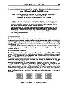
The equations to calculate these frequencies are based on characteristics of the bearing as outlined in table 3. Figure 1 defines each of the parameters (1, 4–6). Table 3. Bearing detect frequency equations. Fault type Fundamental Cage Ball Pass Outer Ball Pass Inner Ball Spin

Defect frequency f  d  f c  s 1  cos   2  D  f  d  f BPO  s N b 1  cos   2 D   fs  d  f BPI  N b 1  cos   2  D  2  fs  d    d  2   1    cos   2  D    D   where f s  shaft rotational frequency

fB 

  contact angle D  Pitch diameter d  ball bearing diameter N b  number of ball bearings

Figure 1. Bearing parameters

4

2.3

Signal Processing Techniques

Signal processing techniques are algorithms that are applied to the signals obtained from the sensor to gain further insight into interpretation of the measured data set. Typically for dynamic components such as bearings and gears, the data measurements are obtained from accelerometers. In general, the sensor output is converted into discrete values as a function of time by the data acquisition system that reads the sensor output. Analysis of the sensor data is very difficult in its raw form. Many signal processing techniques have been developed to process the data into a form that can be more readily interpreted. Signal processing techniques have been developed for a broad range of fields such as communications, imaging, radar and sonar applications. Many of these techniques are applicable to the analysis of the vibrational data from bearings and gears. These techniques are defined in the areas of statistical, time domain, frequency domain and time-frequency domain analysis. 2.3.1 Statistical Analysis Statistical analysis is the mathematical science dealing with the analysis or interpretation of data. Data analysts can use a few straightforward statistical techniques as means of summarizing the collected data from the sensors. These statistical techniques are under the area of descriptive statistics, a methodology to condense the data in quantitative terms. Statistical techniques that are mainly used for alarm purposes in industrial plants are the statistical moments of order two, three and four (8). These are also known as the variance, skewness, and kurtosis. The general equation for the order of moment is as follows:





r 1 N xi  x  N i 1 where r is the order of the moment N is number of data value i is the index of the data value

Mr 

x is the mean value of the data set 2.3.1.1 Mean Mean is the most common measure of a statistical distribution. In this case, mean is the arithmetic average for a set of measurements.

x

1 N

N

x i 1

i

2.3.1.2 Variance Variance is a measure of the dispersion of a waveform about its mean, or is called the second moment of the signal (7).

5

  x  x N

1   N 2

2

i

i 1

2.3.1.3 Skewness Skewness is the statistical moment of the third order normalized by the standard deviation to the third power. This moment indicates the asymmetry of the probability density function or degree of deviation from the symmetry of a distribution (7, 8).



1 N

  x  x N

3

i

i 1

2 1 N  x x  i N   i 1  4 1 N   x x  i N 3 i 1







3/ 2



2.3.1.4 Kurtosis Kurtosis is the fourth statistical moment, normalized by the standard deviation to the fourth power. It is a measure of whether the data is peaked or flat relative to a normal distribution. Most background signal measured by a data acquisition is considered to have a normal distribution in amplitude. The normal distribution has a value of 3 (7, 8).



M4

M2  N



2



N  xi  x i 1



4

2    xi  x   i 1  N





N





  x  x  i 1

4

i

N  2 

1 N 4

2

2

  x  x N

i 1

4

i

2.3.2 Time Domain Analysis

Time domain analysis is usually simpler than frequency domain analysis and less computational. Time domain analysis is based on differentiating good bearings from defective ones by evaluating differences in statistics such as root mean square (RMS), peak value, crest factor and kurtosis. Pattern recognition methods are used to discriminate between good and bad components (2).

6

2.3.2.1 RMS RMS is related to the energy of the signal. The presence of defects are directly detected by the increase in vibration level (7, 8). RMS 

1 N

N

 x  i 1

2

i

2.3.2.2 Maximum Amplitude Value Maximum amplitude value indicates the severity of a bearing defect (7). 2.3.2.3 Peak Level Peak = ½ (max(x(t)) – min (x(t))) 2.3.2.4 Crest Factor Crest factor is a measure of how much impacting is occurring in the time waveform. Impacting in the time waveform may indicate rolling element wear or cavitation (7).

CrestFactor 

PeakLevel RMS

2.3.3 Frequency Domain Analysis

Frequency domain analysis is the scrutiny of data which has been produced by transforming the raw data from the time domain into the frequency domain. In this process, the time series data is transformed to sums of simpler trigonometric functions such as the sine and cosine functions. Through this conversion or transformation, the detection of faults is generally easier, since it improves the signal to noise ratio of the data and the fault signature tends to be more obvious. Signals in general can be divided into two classes: stationary and non-stationary. Signals whose average properties do not change with time and which are independent of the particular sample record used to determine them are said to be stationary. Non-stationary signals are those whose average properties change with time (13). 2.3.3.1 Fourier Analysis Stationary signals are characterized by time-invariant statistical properties, such as the mean value or autocorrelation function. Analysis of stationary signals has largely been based on wellknown spectral techniques such as the Fourier transform, which identifies the constituent frequency components within the signal (12). Traditional data analysis methods such as Fourier analysis are all based on linear and stationary assumptions, i.e., the signal to be processed must be linear and temporally stationary (33). In Fourier analysis, the mathematical process is to transform the time measurements into the frequency domain, where it may be easier to analyze and interpret the sensor measurements.

7

2.3.3.2 Fast Fourier Transform The Fast Fourier Transform (FFT) is an efficient algorithm for calculating the discrete Fourier transform. A discrete Fourier transform converts a series of time discrete measurements into its components in the frequency domain. There are many forms for implementation of the FFT algorithms. The FFT provides the same result as the discrete Fourier transform, but with the main difference being the speed of the overall calculation. For large size of data measurements, this can reduce the computational time by several orders of magnitude. N 1

X k   xn e

 i 2 k

n N

n 0

k  0, , N  1 2.3.3.3 Cepstrum Analysis Cepstrum analysis is a tool for the detection of periodicity in a frequency spectrum. A number of faults tend to cause modulation of the vibration pattern resulting from tooth meshing, and this modulation gives rise to sidebands in the frequency spectrum. Only experience would tell at what point the modulation is serious (10). The principal use of the cepstrum for bearing fault detection is in detecting periodicities associated with bearing frequency harmonics and associated sideband patterns. The cepstrum is the signal processing technique that takes the inverse FFT of the logarithm of the squared magnitude of the Fourier transform of the measured signal.



C p ( )  FFT 1 log  S xx  f  



2.3.4 Time-Frequency Analysis

Time-frequency analysis is an attempt to overcome some of the shortcomings of Fourier analysis. Time-Frequency analysis is a series of signal processing techniques for analyzing signals which are transient in nature or non-stationary. The statistical properties of a nonstationary signal change over time. The time-averaging properties of a non-stationary signal change over time, thus making the time-averaging approach adopted in the Fourier transform ineffective. Time-frequency analysis techniques are methods for analyzing nonlinear and nonstationary data (31). Time frequency techniques decompose one-dimensional time-series signals into a twodimensional plane by exposing the time-dependent variations of characteristic frequencies within the signal, thus presenting a valid and effective tool for non-stationary signal analysis (12). There are many techniques that have been developed to perform time-frequency analysis. Unfortunately, these techniques generate artifacts in cross-term products and the user must be aware of how application of the particular technique will contaminate the results. All the methods are designed to modify the global representation of the Fourier analysis, but they all are

8

limited in one way or the other. Necessary conditions for the basis to represent a nonlinear and non-stationary time series (31): a. complete – guarantees the degree of precision of the expansion b. orthogonal – guarantees positivity of energy and avoids leakage c. local – crucial for non-stationarity, for in such data there is no time scale d. adaptive – adapting to the local variations of the data can the decomposition fully account for the underlying physics The following is a list of time-frequency analysis that will be described: a. Short Time Fourier Transform (STFT) b. Wavelet c. Cohen d. Wigner-Ville e. Choi-Williams f. Zhao-Atlas-Marks g. Hilbert-Huang 2.3.4.1 STFT The STFT is basically the windowing or dividing of the raw data into frames and applying the Fourier transform. This division can be overlapping or non-overlapping of the data. It is an attempt to analyze the non-stationary characteristics of the signal. The resulting twodimensional signal is typically visually displayed as a spectrogram which represents the magnitude squared of the STFT or power variation in the signal over time.

STFT  , f    x(t ) g (t   )e  j 2 fft dt 2.3.4.2 Wavelet Transform The Wavelet transform is a technique similar to the STFT. This technique decomposes the data with various functions that are scaled in amplitude and time. Wavelet Transform is a windowing technique with variable sized regions. The terms “dilations and translations” are the processes applied to the basis function or mother wavelet as it is scaled in width and location as applied to the data set. As with the STFT, it provides the advantage of temporal resolution in addition to the frequency information. Wavelet analysis allows use of long time intervals, where more precise low frequency information is needed and shorter regions where high frequency information is needed (28).

9

1  t   x(t ) *   dt  s  s 

WT ( s, )  2.3.4.3 Cohen

This is a general class of processing that performs analysis in the time and frequency domains. It is an attempt to overcome some of the problems associated with the STFT. It uses bilinear transformation to transform measurement data into the frequency domain while accounting for the non-stationary aspect in the measured data set. The Wigner-Ville, Choi-Williams and ZhaoAtlas-Marks are special implementations of the Cohen technique. Cx  t , f  

 

  A  ,    ,  e

 i 2  t  f  

x

d dt

 

where Ax  ,  is the ambiguity function Ax  ,  





  *

 x  t  2 x



   i 2 t dt t  e  2

  ,  is the kernel function

2.3.4.4 Wigner-Ville Wigner-Ville distribution is a very important quadratic-form time-frequency distribution with optimized resolution in both time and frequency domains. Wigner-Ville is computed by correlating the function with itself, the correlation being a product of the function at a past time with the function at a future time (32). The Wigner-Ville is the Cohen technique with the kernel function defined as unity.   ,   1 Wx  t , f  







 x  t  2  x



*

    i 2 f  d t  e  2

*

where x is the conjugate of x

2.3.4.5 Choi-Willams The Choi-Williams distribution uses the exponential as the kernel function in the Cohen distribution to suppress the cross-term products in the transformation.   ,   e   ,  CWx  t , f    

2

  e 2

2   t  2

2

    x  t   x*  t   e  i 2 f  d d  2  2

10

2.3.4.6 Zhao-Atlas-Marks (Cone-shaped kernel) The Zhao-Atlas-Marks distribution uses a time-lag kernel as the kernel function in the Cohen distribution for suppression of the cross-term product.   t ,  

sin  



ZAM  t , f    

e 2

2

sin  



2     e 2 x  t   x*  t   e  i 2 f  d d  2  2

2.3.4.7 Hilbert-Huang Transform The Hilbert-Huang Transform is another time-frequency analysis technique that combines two processing techniques: Empirical Mode Decomposition (EMD) and the Hilbert transform. The EMD is an algorithm where the signal is decomposed into a set of functions called Intrinsic Mode Functions (IMF) which is almost monocomponent. The IMF represent the simple oscillatory mode versus the harmonic output of the Fourier transform. EMD is empirical, intuitive, direct and adaptive, with a posteriori defined basis derived from the data (33). The Hilbert-Huang Transform is defined as follows (30): 2.3.4.7.1 Empirical Mode Decomposition An IMF is defined as a function that satisfies the following requirements: •

1. In the whole data set, the number of extrema and the number of zero-crossings must either be equal or differ at most by one.

•

2. At any point, the mean value of the envelope defined by the local maxima and the envelope defined by the local minima is zero.

Therefore, an IMF represents a simple oscillatory mode as a counterpart to the simple harmonic function, but it is much more general. Instead of constant amplitude and frequency in a simple harmonic component, an IMF can have variable amplitude and frequency along the time axis. The procedure of extracting an IMF is called sifting. The sifting process: •

1. Identify all the local extrema in the test data.

•

2. Connect all the local maxima by a cubic spline line as the upper envelope.

•

3. Repeat the procedure for the local minima to produce the lower envelope.

The upper and lower envelopes should cover all the data between them. Their mean is m1. The difference between the data and m1 is the first component h1: X(t) – m1 = h1 .

11

Ideally the construction of h1 described above should have made it symmetric and have all maxima positive and all minima negative. Also, h1 should satisfy the definition of an IMF. After the first round of sifting, the crest may become a local maximum. New extrema generated in this way actually reveal the proper modes lost in the initial examination. In the subsequent sifting process, h1 can only be treated as a proto-IMF. In the next step, it is treated as the data, then h1 – m11 = h11 . After repeated sifting up to k times, h1 becomes an IMF, that is h1(k – 1) – m1k = h1k . Then, it is designated as the first IMF component from the data: c1 = h1k . 2.3.4.7.2 The Stoppage Criteria of the Sifting Process The stoppage criterion determines the number of sifting steps to produce an IMF. Two different stoppage criteria have been used traditionally: •

1. The first criterion is proposed by Huang. It is similar to the Cauchy convergence test, and we define a sum of the difference, SD, as SDk

 

T t 0

hk 1 (t )  hk (t )

 t 0 hk21 (t ) T

2

.

Then the sifting process is stopped when SD is smaller than a pre-defined value. •

2. A second criterion is based on the number called the S-number, which is defined as the number of consecutive siftings when the numbers of zero-crossings and extrema are equal or at most differing by one. An S-number is pre-selected, and the sifting process will stop only if for S consecutive times the number of zero-crossings and extrema stay the same, and are equal or at most differ by one.

Once a stoppage criterion is selected, the first IMF, c1, can be obtained. Overall, c1 should contain the finest scale or the shortest period component of the signal. We can, then, separate c1 from the rest of the data by X(t) – c1 = r1. Since the residue, r1, still contains longer period variations in the data, it is treated as the new data and subjected to the same sifting process as described above. This procedure can be repeated to all the subsequent rj’s, and the result is rn – 1 – cn = rn . The sifting process stops finally when the residue, rn, becomes a monotonic function from which no more IMF can be extracted. From the above equations, we can induce that

12

n

X (t )   c j  rn j 1

Thus, a decomposition of the data into n-empirical modes is achieved. The components of the EMD are usually physically meaningful because the characteristic scales are defined by the physical data. 2.3.4.7.3 Hilbert Transform Having obtained the intrinsic mode function components, the instantaneous frequency can be computed using the Hilbert Transform. After performing the Hilbert Transform on each IMF component, the original data can be expressed as the real part in the following form : n

X (t )  Real   a j (t )e

i  w j (t )

dt .

j 1

3. Gears Gear vibration monitoring employs the same techniques as bearing vibration analysis. The development of diagnostic indicators or algorithms is further along for gears than compared to bearings. As in bearings, it uses statistical signal and spectral analysis (27). Many of the diagnostic indicators/algorithms use spectral comparison where the baseline power (magnitude squared) spectrum is taken under well defined, normal operating conditions with the machine in known good condition. This ‘baseline’ spectrum is used as a reference for subsequent power spectra taken at regular intervals throughout machine life (26). Vibrational measurements are one of the common sources of data for gear evaluation. This is conducted through the use of accelerometers. Based on various controlled experiments the accelerometer location and orientation appear to be critical in effectively detecting damage early (19). A survey of world-wide airworthiness-related accidents of civil fleet helicopters between 1956 and 1986 was performed. Breakdown of transmission related accidents by component is outlined in the table 4. Gears have a significant impact as the source of major accidents as compared to bearings. Approximately 19% of all transmission related helicopter accidents were caused by gear failures (26).

13

Table 4. Summary of helicopter accidents Component Tail rotor drive shaft Gears Main rotor drive shaft Lubrication system Main gearbox input shaft Bearings Freewheels Cooling fan drive Unknown

3.1

Percentage of accidents 31.9 19.1 14.9 8.5 8.5 4.3 4.3 4.3 4.3

Diagnostic or Signal Enhancement Techniques

Interpretation and correlation of vibrational analysis results are difficult, even for the most experienced personnel. Many diagnostic indicators or condition indicators have been developed over the last few decades. These indicators typically use a combination of statistical and advanced signal processing techniques. Defects or damage will increase the machinery vibration level. Through vibrational measurements, the health of the monitored machine is contained in this vibration signature. Hence, the new or current vibration signatures could be compared with previous signatures to determine whether the component is behaving normally or exhibiting signs of failure. In practice, such comparisons are not effective. Due to the large variations, direct comparison of the signatures is difficult. Instead, a more useful technique involves the extraction of features from the vibrational signature data. Ideally, these features are more stable and better behaved than the raw signature data itself. These features also provide a reduced data set for the application of pattern recognition and tracking techniques. 3.2

Time Synchronous Average (TSA)

TSA is a rather common method for early detection of failure in gears. By synchronizing the vibration signal with the rotation of a particular gear and evaluating the ensemble average over many revolutions with the start of each frame at the same angular position, a signal, called time synchronous average is obtained, which in practice contains only the components which are synchronous with the revolution of the gear. This process reduces the effects of all other sources, including other gears, and noise. TSA is a signal processing technique that is used to extract repetitive signals from additive noise. In this technique, a signal that is synchronous with the shaft rotation provides the registration mark that is used to delineate the beginning data point associated with every shaft rotation. A number of data sets for individual shaft rotations are averaged together to a single representation of the bearing data set. Increasing the number of averages should improve the average by averaging out more of the non-synchronous components and enhancing the synchronous components, but it is more computationally intensive (16).

14

The TSA is used in conjunction with many of the diagnostic indicators as defined in the following text. Terminologies used to describe these algorithms are somewhat vague and do not necessarily have clear definitions. Two of these terms are residual and difference. Residual consist of the TSA signal with the primary meshing, shaft components and their harmonics removed. What is not clear is how many harmonics to remove for the primary mesh and shaft components. Favorable results have been obtained by high pass filtering the data about some frequency and only removing the meshing frequency and all harmonics. The residual is used in NA4 and NA4* diagnostic indicator. Difference is the removal of the regular meshing components from the TSA. The regular meshing components consist of the shaft frequency and its harmonics, the primary meshing frequency and its harmonics, and the first order sidebands. This is similar to Residual with the addition of the sidebands of the primary meshing frequency. The difference is used in FM4 and M6 diagnostic indicator (16). 3.3

FM0

FM0 is an indicator of major faults in a gear mesh. Localized faults tend to increase in Peak-toValley faster than the magnitude of meshing harmonics. It is defined as the ratio of the peak-topeak level of the signal average to the sum of the RMS levels of the meshing frequency and its harmonics (20, 23). The following are some of its characteristics as defined by R. M. Stewart (the developer) (18): 1. It detects changes in the average of a significant kind. 2. It is a global technique and will react to changes occurring anywhere in the frequency span of the average. 3. It will react to a change in only one frequency (a fairly common occurrence with gearbox faults) 4. It is non-dimensional in a way that makes it relatively insensitive to load changes, but not speed. 5. It is also fairly tolerant to accelerometer positioning error . The equation for FM0 is (16, 17, 20, 22, 24, 26):

15

FM 0 

 Peak  to  Peak TSA n

 A f  i 1

i

where

 Peak  to  Peak TSA is the peak-to-peak value of the TSA waveform n

 A  f  is amplitude of the gear mesh fundamental and harmonics in the i 1

i

frequency domain

3.4

FM4

FM4 is an indicator of changes in the vibration pattern resulting from damage to a single tooth. In this routine, the regular meshing components are filtered from the signal average obtained from the TSA operation and two statistical operations, standard deviation and kurtosis performed on the difference signal. The difference signal is constructed by removing the shaft frequency and its first few harmonics, the meshing frequency and its harmonics, and their first order side bands (20, 23). An important problem in gearbox monitoring is how to treat the gearbox, which operates over a wide range of loads and speeds and is not important enough to warrant holding in store a sufficient number of signatures. The concept behind the number is that the average of a perfect gear will contain only shaft order harmonics that produce an even pattern with the average, and that many of the coefficient values in the FFT of the average appear solely in order to the make one tooth different from its neighbors. If one, therefore, takes an average and then subtracts one from the ‘regular’ components, and then reconstructs a ‘regular’ average, and finally subtracts one from the other (hence the name ‘bootstrap reconstruction’), once might end up with some useful information. The main problem is, of course, connected with choice of harmonics which constitute the ‘regular’ set (18). The equation for FM4 is (16, 17, 19, 20, 22, 24, 26, 27): N

FM 4 



N  di  d i 1



4

2   d d  i    i 1  N





2

where d is difference signal d is mean value of difference signal

16

3.5

NA4

NA4 is an indicator used to detect the onset of damage, but it also continues to react to the damage as it increases. This is similar to FM4, but the residual signal is constructed by removing regular meshing components from the original signal while keeping the first order sidebands in the residual signal. A residual signal is created by removing only the meshing frequency components from the vibration signal and dividing the fourth statistical moment by the current run-time-averaged variance, i.e., the averaged variance of all signals from the start of the run up to the present (21, 23). The equation for NA4 is (16, 17, 19, 22, 24, 27): N

NA4 



N  ri  r i 1

 1  M



4

2 N r r    ij j   j 1  i 1 



M



2

where r is residual signal r is mean value of residual signal N is the total number of time points in the time record i is data point number in time record M is the current time record number in run ensemble j is time record index in run ensemble 3.6

M6

M6 is an indicator of fault in the gears. The algorithm is similar to the application of kurtosis to detection of gear faults. In this algorithm, the sixth moment of the difference signal is normalized by the variance raised to the third power (15, 16, 19, 24). N

M6 



N 2  di  d i 1







2   d i  d   i 1  N

6

3

where d i is the difference signal d is the mean value of difference signal i is data point index N is number of data points

17

3.7

NB4

NB4 is similar to the NA4 indicator. NB4 uses the same equation as NA4 except that the residual signal is replaced by the envelope of the signal bandpassed about the mesh frequency. Using the Hilbert transform, a complex time signal is created in which the real part is the bandpass signal, and the imaginary part is the Hilbert transform of the signal. The envelope is the magnitude of this complex time signal, and represents an estimate of the amplitude modulation present in the signal due to the sidebands (21). The equation for NB4 is (16, 17, 19, 22, 24, 27): N

NB 4 



N  Ei  E i 1

 1  M



4

2 N E  E   ij j   j 1  i 1  M





2

where E is the envelope of the band-passed signal E(t) = (A(t)) 2  H [ A(t )]2 A(t ) is the band-passed signal H [ A(t )] is the Hilbert trasnsform of the band-passed signal 3.8

FM4*

FM4* is an improvement on the FM4 algorithm. In this case, the numerator is calculated the same way as in FM4. Then, the denominator is replaced with the run ensemble average as defined in NA4* (24). 3.9

NA4*

NA4* is used to overcome the associated problem of NA4. In gears, as the damage progresses from localized to distributed, the variance of the kurtosis increases. The NA4 algorithm uses the kurtosis. Since the kurtosis is normalized by the variance, this results in the kurtosis decreasing to normal values even with damage. To overcome this problem, in NA4*, the data record is normalized by the squared variance for a good gearbox (24). 3.10 NB4*

NB4* is an improvement on the NB4 algorithm. In this case, the numerator is calculated the same way as in NB4. The denominator is replaced with the run ensemble average as defined in NA4* (24). 3.11 NP4

NP4 is similar to the other condition indicators in the sense that it is normalized by the variance. The difference is that the time domain power signal is derived from the Wigner-Ville distribution 18

and does not require the comparison of the undamaged (baseline) gear vibration signal with the acquired gear vibration signal. An advantage of this technique is that it avoids the need to interpret the Wigner-Ville analysis (25).

1 NP 4  N

 P  ti   P     3    i 1   4

N

where P (t )   W (t , f ) df

4. Summary of the Results Obtained by Researchers in the Application of the Diagnostic Indicators The following results were noted from the diagnostic techniques in the literature: •

RMS, Energy Ratio, Energy Operator, Kurtosis, and NA4 are very sensitive to torque fluctuations and thus may not be effective (19).

•

Generally the RMS value of the vibration signal is a very good descriptor of the overall condition of the gearbox. Its value increases as tooth failure progresses. RMS does not increase with the isolated peaks in the signal; consequently this parameter is not sensitive to incipient tooth failure (22).

•

FM4, NA4, NB4, NA4*, NB4* were found to be more robust for diagnosis of initiation and progress of damage. NA4* is less likely to ignore existing damage (27).

•

FM4, NA4, NB4, and NB4* are good indicators of initial pitting only (27).

•

Most effective (in decreasing order) were M6A*, FM4* and NB4. They are sensitive enough to pick up damage while not being overly sensitive to torque fluctuations (19).

•

NP4 deteriorates as the severity of the damage increases on multiple gear teeth (25).

•

Crest factor indicates damage in an early stage. As damage progresses the RMS value of the vibration signal increases its value and the crest factor decreases (22).

•

Kurtosis computation has an inherent characteristic of being self-limited, which reduces the scope of many kurtosis-based applications. The key to developing an effective application lies in producing an appropriately tailored signal (27).

•

Wigner-Ville has two problems related to processing artifacts such as cross-terms and aliasing (28).

19

•

In terms of the time-frequency analysis, the best resolutions are provided by Zhao-AtlasMarks, Choi-Williams, and Cohen in that order, but require greater computation time compared to the STFT (11).

5. Automation of Fault Detection The traditional methods for fault diagnosis are categorized as pattern classification, knowledgebased inference, and numerical modeling. Pattern classification and knowledge-based inference techniques are used in the industry. In these two methods, a human expert looks for particular patterns in the vibration signature that might indicate the presence of a fault in the bearing. Alternatively, numerical modeling which employs statistical analysis and Artificial Neural Networks are used in automated fault detection systems (14). The majority of diagnostic techniques have some ability to indicate the presence of damage. Each technique has associated strengths and limitations. A technique may be very good at detecting particular faults but weak, or useless, at detecting others. Any one technique is generally insufficient for detecting all various types of damage. Model-based techniques offer a fundamentally different approach to detection. The fundamental idea is that the technique is trained to recognize signals from a healthy system and indicate when the vibration deviates from this nominal condition. Neural networks are the most commonly used for model-based diagnostics. A neural network is defined as a massively parallel distributed processor that has a natural propensity for storing experiential knowledge and making it available for use. It possesses two fundamental properties: (1) the network obtains knowledge through a learning process, and (2) the interneuron connection strengths or weights are used to retain the knowledge. In general, a neural network damage detection system does not process the vibration signal directly. Instead, it takes as input the results of various processing techniques, learning how the techniques behave in the presence of healthy and faulty data (17). Artificial neural networks can approximate almost any non-linear function, which provides the fundamental fact that it is possible to model the non-linear dynamics of gearboxes by an appropriate neural network (35). Self-organizing feature maps (SOFM) are a paradigm of neural networks to map a highdimensional space on to a low-dimensional feature map. This approach preserves with most of the topological relationships of the signal domain so that humans can more readily understand the high-dimensionality data that is typically hard to comprehend. The advantage of SOFM, as opposed to traditional clustering methods, is to visualize the complicated cluster distribution on the low-dimensional feature map without setting the number of clusters in advance (35). This is a nonlinear projection method that efficiently maps different characteristic features into the

20

clusters on the map without any explicit modeling of the system. In this approach SOFM to be effective, feature selection is critical (36).

6. Summary There has been much written on the development of diagnostic techniques for dynamic components based on decades worth of research. Most of the measured data is obtained from accelerometers that provide vibrational information. The diagnostic techniques can be categorized into several domains: statistical, time, frequency and time-frequency domains. Most of the diagnostic techniques are basic signal processing techniques that have been developed for other fields such as communication, radar and image processing. The basic signal processing techniques are common for both the bearing and gear fault detection. Development of the bearing fault equations provides for an easier fault detection process. Since the gear has been identified as the major component that results in accidents, there has been development in terms of specific signal enhancements for improved detection of gear faults. All the research has been conducted only on particular test situations, which do not necessary cover all the degradation mechanisms. To improve the confidence level associated with the detection of a fault, these diagnostic indicators will have to be combined. Artificial Neural Network is a possible solution of these fault detection, since an individual fault detector probably does not have a low false alarm probability, nor a sufficient highly probability of detection by itself.

21

7. References 1. Howard, Ian. A Review of Rolling Element Bearing Vibration Detection, Diagnosis and Prognosis; DSTO-RR-0013; Aeronautical and Maritime Research Laboratory: Airframes and Engines Division. 2. Chuang, Jason C. H.; Sosseh, Raye A. A Survey Report of Acoustic Emission Used in Roller Bearing Fault Detection. School of Aerospace Engineering, Georgia Institute of Technology, February 1, 1998. 3. Bouzaouit, A.; Hadjadi, A. E.; Chaib, R. Statistical Study on the Bearing’s Degradation. Asian Journal of Information Technology 2007, 6, 891–895. 4. McInerny, S. A.; Dai, Y. Basic Vibration Signal Processing for Bearing Fault Detection. IEEE Transactions on Education February 2003, 46 (1), 149–156. 5. Li, Bo; Goddu, Gregory; Chow, Mo-Yuen. Detection of Common Motor Bearing Faults Using Frequency-Domain Vibration Signals and a Neural Network Based Approach. Proceedings of the American Control Conference, June 1998, 2032–2036. 6. Orhan, Sadettin; Akturk, Nizami; Celik, Veli. Vibration Monitoring for Defect Diagnosis of Rolling Element Bearings as a Predictive Maintenance Tool: Comprehensive Case Studies. NDT&E International 39 2006, 293–298. 7. Lee, Hong-Hee; Nguyen, Ngoc-Tu; Kwon, Jeong-Min. Bearing Diagnosis Using TimeDomain Features and Decision Tree. School of Electrical Engineering, University of Ulsam, Korea. 8. de Almeida, Rui Gomes Teixeira; da Silva Vicente, Silmara Alexandra; Padovese, Linilson Rodrigues. New Technique for Evaluation of Global Vibration Levels in Rolling Bearings. Shock and Vibration 9 2002, 225–234. 9. Heng, R.B.W.; Nor, M.J.M. Statistical Analysis of Sound and Vibration Signals for Monitoring Rolling Element Bearing Condition. Applied Acoustics 1998, 53 (1–3), 221–226. 10. Randall, R. B. Cepstrum Analysis and Gearbox Fault Diagnosis. B&K Instruments, Inc., Application Notes. 11. Randall, R. B.; Gao, Y.; Ford, R. A Comparison of Time-Frequency Distributions Applied to Bearing Diagnostics. Proceedings of First Australasian Congress on Applied Mechanics, February 21–23 1996. 12. Gao, R. X.; Yan, R. Non-stationary Signal Processing for Bearing Health Monitoring. Int. J. Manufacturing Research 2006, 1 (1), 18–40. 22

13. Sawalhi, Nader. Diagnostics, Prognostics and Fault Simulation For Rolling Element Bearings. The University of New South Wales, School of Mechanical and Manufacturing Engineering, Australia, Doctor of Philosophy thesis, 2007. 14. Ghafari, Shahab Hasanzadeh. A Fault Diagnosis System for Rotary Machinery Supported by Rolling Element Bearings, University of Waterloo, Mechanical Engineering, Waterloo, Ontario, Canada, Doctor of Philosophy thesis, 2007. 15. Lebold, Mitchell; McClintic, Katherine; Campbell, Robert; Byington, Carl; Maynard, Kenneth. Review of Vibration Analysis Methods For Gearbox Diagnostics and Prognostics. Proceedings of the 54th Meeting of the Society for Machinery Failure Prevention Technology, May 1–4, 2000. 16. Dalpiaz, G.; Rivola, A.; Rubini, R. Effectiveness and Sensitivity of Vibration Processing Techniques for Local Fault Detection in Gears. Mechanical Systems and Signal Processing 2000, 14, 387–412. 17. Samuel, Paul D.; Pines, Darryll J. A Review of Vibration-based Techniques for Helicopter Transmission Diagnostics. Journal of Sound and Vibration 282 2005. 18. Stewart, R. M. Some Useful Data Analysis Techniques for Gearbox Diagnostics. Institute of Sound and Vibration Research. Proc. Of Meeting on Applications of Time Series Analysis, July 1977, 8.1-19. 19. Decker, H.; Lewicki, D. Spiral Bevel Pinion Crack Detection in a Helicopter Gearbox; ARL-TR-2958; NASA Glenn: Cleveland, OH, 2003. 20. Zakrajsek, James J. An Investigation of Gear Mesh Failure Prediction Techniques; AVSCOM 89-C-005; November 1989. 21. Zakrajsek, James J.; Handschush, Robert F.; Decker, Harry J. Application of Fault Detection Techniques to Spiral Bevel Gear Fatigue Data; ARL-TR-345; NASA Glenn, Cleveland, OH, 1994. 22. Vecer, P.; Kreidl, M.; Smid, R. Condition Indicators for Gearbox Condition Monitoring Systems. Acta Polytechnica 2005, 45 (6), 35–43. 23. Choi, Sukhwan; Li, C. James. Estimate Gear Tooth Transverse Crack Size from Vibration by Fusing Selected Gear Condition Indices. Measurement Science and Technology 2006, 17, 2395–2400. 24. Decker, Harry. Crack Detection for Aerospace Quality Spur Gears; ARL-TR-2682; NASA Glenn: Cleveland, OH, 2002. 25. Polyshchuk, V. V.; Choy, F. K.; Braun, M. J. Gear Fault Detection with Time-Frequency Based Parameter NP4. International Journal of Rotating Machinery 2002, 8 (1), 57–70.

23

26. Forrester, B. David. Advanced Vibration Analysis Techniques for Fault Detection and Diagnosis in Geared Transmission Systems. Swinburne University of Technology, Australia, Doctor of Philosophy thesis, 1996. 27. Rao, V. Bhujanga. Kurtosis as a Metric in the Assessment of Gear Damage. The Shock and Vibration Digest 1999, 31 (6), 443–448. 28. Cao, Yingfang. Adaptability and Comparison of the Wavelet-Based with Traditional Equivalent Linearization Method and Potential Application for Damage Detection. North Carolina State University, Mechanical Engineering, Master thesis, 2002. 29. Armstrong, Robert A. Fault Assessment of a Diesel Engine Using Vibration Measurements and Advanced Signal Processing. Naval Postgraduate School, Master thesis, 1996. 30. Huang, Norden E.; Shen, Samuel S. P. Hilbert-Huang Transform and Its Applications. Interdisciplinary Mathematical Sciences 2008, 5, 2–14. 31. Huang, Norden E.; Shen, Zheng; Long, Steven R.; Wu, Manli C.; Shis, Hsing H.; Zheng, Quanan; Yen, Nai-Chyuan; Tung, Chi Chao; Liu, Henry H. The Empirical Mode Decomposition and the Hilbert Spectrum for Nonlinear and Non-stationary Time Series Analysis. Proc. Royal Society London 1998, 454, 903–495. 32. Loutridis, S. J. Instantaneous Energy Density as a Feature for Gear Fault Detection. Mechanical Systems and Signal Processing 20 2006. 33. Raja, J. Emerson; Loo, C. K.; Rao, M.V.C. The Necessity of a Non-linear & Non-stationary Data Processing in Engineering and the New Hilbert Huang Transform (HHT). Pay Attention, Gain Understanding December 2007, 1 (3). 34. Wu, Biqing; Saxena, Abhinav; Khawaja, Taimoor Saleem; Patrick, Romano; Vachtesevanos, George; Sparis, Panagiotis. An Approach to Fault Diagnosis of Helicopter Planetary Gears. Georgia Institute of Technology. 35. Liao, G.; Liu, S.; Shi, T.; Zhang, G. Gearbox Condition Monitoring Using Self-Organizing Feature Maps. Proceedings of the Institution of Mechanical Engineering, Part C, Journal of Mechanical Engineering Science, Vol. 218, November 1, 2004, 119–129. 36. Saxena, Abhinav; Saad, Ashraf. Fault Diagnosis in Rotating Mechanical Systems Using Self-Organizaing MAPS. School of Electrical and Computer Enigeering, Georgia Institute of Technology.

24

NO. OF COPIES ORGANIZATION 1

1 CD

1

1

NO. OF COPIES ORGANIZATION

ADMNSTR DEFNS TECHL INFO CTR ATTN DTIC OCP 8725 JOHN J KINGMAN RD STE 0944 FT BELVOIR VA 22060-6218

1

NASA GLENN ATTN RDRL VTP H DECKER BLDG 23 RM W121 CLEVELAND OH 44135-3191

1

NASA GLENN ATTN RDRL VTP B DYKAS BLDG 05 RM W213B CLEVELAND OH 44135-3191

1

US GOVERNMENT PRINT OFF DEPOSITORY RECEIVING SECTION ATTN MAIL STOP IDAD J TATE 732 NORTH CAPITOL ST NW WASHINGTON DC 20402

1

US ARMY RSRCH LAB ATTN RDRL CIM G TECHL LIB T LANDFRIED BLG 4600 ABERDEEN PROVING GROUND MD 21005-5066

9

US ARMY RSRCH LAB ATTN RDRL CIM L TECHL PUB ATTN RDRL CIM L TECHL LIB ATTN RDRL SER E A BAYBA ATTN RDRL SER E R DEL ROSARIO ATTN RDRL SER E G MITCHELL ATTN RDRL SER E C LY ATTN RDRL SER E K TOM ATTN RDRL SER E D WASHINGTON ATTN IMNE ALC IMS MAIL & RECORDS MGMT ADELPHI MD 20783-1197

OFC OF THE SECY OF DEFNS ATTN ODDRE (R&AT) THE PENTAGON WASHINGTON DC 20301-3080 US ARMY RSRCH DEV AND ENGRG CMND ARMAMENT RSRCH DEV & ENGRG CTR ARMAMENT ENGRG & TECHNLGY CTR ATTN AMSRD AAR AEF T J MATTS BLDG 305 ABERDEEN PROVING GROUND MD 21005-5001 PM TIMS, PROFILER (MMS-P) AN/TMQ-52 ATTN B GRIFFIES BUILDING 563 FT MONMOUTH NJ 07703

1

US ARMY INFO SYS ENGRG CMND ATTN AMSEL IE TD A RIVERA FT HUACHUCA AZ 85613-5300

1

COMMANDER US ARMY RDECOM ATTN AMSRD AMR W C MCCORKLE 5400 FOWLER RD REDSTONE ARSENAL AL 35898-5000

3

US ARMY RDECOM-ARDEC ATTN RDAR WSF A G GARCIA ATTN RDAR WSF A M LOSPINUSO ATTN RDAR WSF A D MARSTON BLDG 91 PICATINNY NJ 07806

2

US ARMY TARDEC ATTN RDTA RS C BECK ATTN RDTA RS K FISHER MS# 204 6501 E 11 MILE RD WARREN MI 48397-5000

TOTAL: 24 (1 ELEC, 1 CD, 22 HCS)

25

INTENTIONALLY LEFT BLANK.

26