2008 IEEE Swarm Intelligence Symposium St. Louis MO USA, September 21-23, 2008
Swarm Intelligence Based Optimization and Control of Decentralized Serial Sensor Networks Kalyan Veeramachaneni, Lisa Osadciw
Department of Electrical Engineering and Computer Science Syracuse University, Syracuse NY-13244 kveerama,
[email protected] Abstract – In this paper threshold design and hierarchy management of serial sensor networks employed for distributed detection is accomplished using a hybrid of ant colony optimization and particle swarm optimization. The particle swarm optimization determines the optimal thresholds, decision rules for the sensors. The ant colony optimization algorithm determines the hierarchy of sensor decision communication, affecting the accuracy. The problem of hierarchy management is known as “who reports to whom?” problem in sensor networks. The new algorithm is tested on a suite of 10 heterogeneous sensors. Probabilistic measures including probability of error and Bayesian risk are adopted to evaluate the performance of the sensor network. The new sensor management methodology is compared to (a) Static hierarchy network, (b) a network with the best sensor at the top of the hierarchy and (c) Incrementally best hierarchy. Results show 40% performance improvements in terms of Bayesian risk value. Keywords: Distributed detection, sensor networks, ant colony optimization, particle swarm optimization
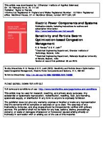
I. INTRODUCTION Multi-sensor networks consist of sensors employed to measure and detect the presence or absence of phenomena. Some phenomena of interest and applications of these networks include intrusion detection systems using biometrics, detection of forest fires, detection of chemical, biological and nuclear agents, detecting faults on an aircraft engine, and detecting cracks in a pipeline [10, 12, 13]. Each sensor has communication capabilities integrated in its design and sends the information that it has processed/measured to the next node in the network. The final node that receives the information does the final situation assessment. An alternative arrangement known as parallel network employs a central fusion processor to which all sensors communicate. The serial and parallel architectures are shown in figure 1. For sensor networks with limited communication channels, the former architecture is more desirable. In a distributed/decentralized detection framework, each sensor applies a threshold to its observation and gives a decision regarding the presence or absence of phenomena. Under binary hypothesis-testing problem sensors make a hard decision (a binary digit 0 or 1 for binary hypothesis) and send their decision to the neighboring node. The final node in the series makes the final decision. This type of
framework minimizes the bandwidth/power usage of a sensor network by transmitting a single bit, representing the decision, to the next node. Due to this thresholding of the measurement, accuracy is compromised for the sake of bandwidth. Accuracy is defined using the two types of errors the network can make in detection of the hypothesis i.e., Type I and II. In Type I error hypothesis H1 is declared while H0 is present. In Type II hypothesis H0 is declared when H1 is present. Loss in accuracy can be minimized by carefully designing these thresholds (decision rules). Sensors are modeled using the likelihood conditional probabilities assumed under both the hypotheses. For serial networks, Tang et al. formulated the “optimal thresholding” problem as deterministic, non-linear multi stage control problem [1] and applied min-H algorithm from optimal control theory. In [4], a person-by-person optimal solution and a Gauss-seidal iterative procedure is presented for solving the problem. Both the approaches have a tendency to get stuck at local optima or a saddle point. Tang et al. suggest running their algorithm multiple times in order to achieve global optima [1]. The use of these approaches is also limited for homogeneous networks, i.e. “known signal in additive white Gaussian noise” and sensors with strictly concave receiver operative characteristic curves. With higher computational power that is available now, the problems in parallel architecture have been revisited by researchers in [10, 11, 14]. Veeramachaneni et al. in [10, 14] use a particle swarm optimization based approach to minimize the risk for a single-threshold parallel network. Saeed et al. use a Genetic algorithm to minimize the Bayesian risk for a multi-threshold parallel network. In this paper, we revisit the problems in serial architectures. We present a particle swarm optimization (PSO) algorithm to solve the threshold problem for serial networks. The aforementioned schemes (in previous paragraph) assume fixed hierarchy, i.e., the sequence of detectors. For a fixed sequence, the threshold for each sensor measurement is designed. The performance of the decentralized detection network is significantly affected by the sequencing of the sensors, i.e., ‘who reports to whom?’ even when the thresholds are optimized for the sequence [1, 2, 3, 4].
978-1-4244-2705-5/08/$25.00 ©2008 IEEE Authorized licensed use limited to: Syracuse University Library. Downloaded on June 23, 2009 at 09:09 from IEEE Xplore. Restrictions apply.
S4
b
4
S1
S2
b1
b2
S3
b3
S4 b
4
b3
b1
S3
b2
S2
S1
u0
S6
S5
b5
u0
F u s io n C e n te r
Figure 1 Decentralized Sensor Network Architectures: Parallel and Serial
A joint optimization and control algorithm using particle swarm optimization and ant based control and optimization, called ABC-PSO, is proposed in this paper. As the number of sensors increases the number of combinations in which the sensors can be sequenced increase exponentially. For example, for 5 sensors there are 120 possible sequences, for 8 sensors there are 40320 and for 10 there are 3628800. Even if it is assumed that optimal thresholds are available for each of the sequence, which is an intractable problem itself [4], the search for the optimal sequencing will be intractable as the number of sensors increase. In this paper an ant colony optimization algorithm is coupled with the PSO algorithm to arrive at an optimal sequence and the optimal thresholds for a given sequence. Ants construct the sequence and the PSO identifies the thresholds and achieves the minimum error for the sequence. This is fed back to ants to help them move in the search space and identify better sequences. Ants use probabilistic rules to search for a sequence. The probabilistic rules are designed to search for the optimal sequence in sensor network. The algorithm is compared with two different strategies. One of the strategies commonly used by the practitioners is using the best sensor at the end [1, 4]. In following subsections, we formulate the problem for a decentralized serial detection network. Section II presents the particle swarm optimizer. Section III describes the ant based optimization approach. The probabilistic transition rule designed for the problem is detailed. The combination of ant colony optimization and PSO as applied to the sensor management problem in serial networks is presented in Section IV. The results for a sensor network test bed are presented in Section V. The results are compared with “Static hierarchy”, “Best Sensor Last” and “Incrementally best hierarchy” design methodologies. Conclusions and future work are presented in Section VI. A. Problem Formulation Consider a binary hypothesis-testing problem. A binary decision ‘1’ is sent indicating the presence of the H1 and ‘0’ indicating the presence of H0. All the detectors are
connected in series and receive direct observations of the common phenomena denoted as xi . Sensor observations are conditioned over both the hypotheses and are assumed independent in this paper, implying n
P ( x1 , x2 ........ xn | H h ) = ∏ P ( xi | H h ) .
(1)
i =1
Each detector makes a decision bi based on its own observation xi and the decision transmitted to it from the previous detector denoted as bi −1 here. Hence each detector has two thresholds λ i = {λ bi −1 = 0 , λ bi −1 =1} that it uses to apply to its measurement and arrive at a decision. λ bi −1 = 0 is used if the incoming decision from the previous sensor is ‘0’, i.e., bi −1 = 0 , otherwise the threshold λ bi −1 =1 is used. The final node receives the decision from its predecessor and forms the global decision, i.e., bn = g n (bn −1 , λ n ) where uo = bn (2) Hence inherently each sensor fuses its own information with the previous sensor. Design of gi involves the design of λ i . The two errors that the sensor network can make are (3) e1 = P ( H 0 ) P ( u o = 1 | H 0 )
= P( H 0 )
[ bn −1 ]
P (bn = 1 | [bn −1 ], H 0 ) P ([bn −1 ] | H 0 )
Expanding equation (3) will result in e1 = P ( H 0 ) e1 = P ( H 0 )
P ( bn = 1 | bn −1 = 1, H 0 ) P ( bn −1 = 1 | H 0 ) + P ( bn = 1 | bn −1 = 0, H 0 ) P (bn −1 = 0 | H 0 ) P ( xn > λ bn −1 =1 | H 0 ) P (bn −1 = 1 | H 0 ) + P ( xn > λ bn −1 = 0 | H 0 ) P (bn −1 = 0 | H 0 )
and e2 = P ( H 1 ) P ( u o = 0 | H 1 )
= P( H1 ) e2 = P ( H 1 ) e2 = P ( H 1 )
. (4)
[ bn −1 ]
(5)
P ( bn = 0 | [bn −1 ], H 1 ) P ([bn −1 ] | H 1 )
P ( bn = 0 | bn −1 = 1, H 1 ) P ( bn −1 = 1 | H 1 ) + P ( bn = 0 | bn −1 = 0, H 1 ) P ( bn −1 = 0 | H 1 ) P ( x n ≤ λ bn −1 =1 | H 1 ) P ( bn −1 = 1 | H 1 ) + P ( x n ≤ λ bn −1 = 0 | H 1 ) P ( bn −1 = 0 | H 1 )
Authorized licensed use limited to: Syracuse University Library. Downloaded on June 23, 2009 at 09:09 from IEEE Xplore. Restrictions apply.
(6)
Notice that (4) and (6) are recursive and P(bn −1 = 0 | H1 ) and P(bn −1 = 1 | H 0 ) can be obtained by replacing ‘n’ by ‘n-1’ in (6) and (4) respectively. This can be done until n=2. Similar expressions can be obtained for P(bn −1 = 1 | H1 ) and P(bn −1 = 0 | H 0 ) and subsequent recursion will give these values for n-2, n-3 …. 2. Due to space limitations the entire derivation is not given in this paper. When n=1 the errors are calculated using P(b1 = 0 | H1 ) = P ( x1 > λ 1 | H 0 ) (7)
P(b1 = 1 | H 0 ) = P( x1 ≤ λ 1 | H 0 ) (8) The objective of the design of the thresholding scheme for the decentralized detection networks is to minimize the two errors as in (9) min e1 λ1 ,λ 2 ,..... λ n
min
λ1 ,λ 2 ,..... λ n
e2 .
(10)
A weighted sum of these two errors known as Bayesian risk as in (11) min E= w1 × e1 + w2 × e2 λ1 ,λ2 ,..... λn
is minimized. The sum of the two weights is equal to 1, i.e., w1 + w2 = 1 . (12) B. “Who reports to whom?” Sequencing of detectors significantly affects the performance of the serial networks [1, 4]. This is known as ‘who reports to whom?” problem. Engineers usually have the best detector make the final decision. The rest of the sensors are arranged in random fashion. Examples have been presented in [3] which show that this ordering is not optimal. Different sequences have different performances. Performance significantly varies even if the underlying thresholds are fully optimized for a particular sequence. Also, for different values of w1 different sequences can be optimal. Formally this problem is stated as follows. Given a set of nodes N, i.e., S={1, 2, 3, ..N-1, N}, and w1, find the optimal sequence d ( S ) = [d1 , d 2 ,.........d n ] such that ‘E’ (11) is minimized. In this paper, we propose using an ant colony based approach to achieve the optimal communication hierarchy. Table 1: Number of Sequences as a function of number of sensors
.
# Sensors
# Sequences
5 6 8 10
120 720 40320 3628800
II. PARTICLE SWARM OPTIMIZATION The particle swarm optimization algorithm, introduced by Kennedy and Eberhart in 1995 [5], is derived from simulation of social behavior of individuals. The individuals, called particles henceforth, are flown through the multi-dimensional search space, with each particle representing a possible solution to the multidimensional problem. The movement of the particles is influenced by two factors: as a result of the first factor, each particle stores in its memory the best position visited by it so far, called pbest and experiences a pull towards this position as it traverses through the search space. As a result of the second factor, the particle interacts with all the neighbors and stores in its memory the best position visited by any particle in the search space and experiences a pull towards this position, called gbest. The first and the second factors are called cognitive and social components respectively. After each iteration the pbest and gbest are updated if a more dominating solution (in terms of performance) is found, by the particle and by the population respectively. This process is continued iteratively until either the desired result is achieved or the computational power is exhausted. Formally, the PSO formulae define each particle in the D-dimensional space as X i = ( xi1 , xi 2 ,...., xiD ) where the subscript i represents the particle number and the second subscript is the dimension. The memory of the previous best position is represented as Pi = ( pi1 , pi 2 ,...., piD ) and a
velocity
along
Vi = ( vi1 , vi 2 ,...., viD ) .
each dimension as After each iteration, the
velocity term is updated and the particle is pulled in the direction of its own best position, Pi and the global best position, Pg, found so far. This is apparent in the velocity update equation, (13). (t ) (t) (t) Vid(t+1) = ω × Vid + U [0,1] ×ψ 1 × ( pid − xid ) + (13) U [0,1] ×ψ 2 × ( p gd ( t ) − xid ( t ) ) where U[0,1] is a sample from a uniform random number generator, t represents a relative time index, ψ 1 is a weight determining the impact of the previous best solution, and ψ 2 is the weight on the global best solution’s impact on particle velocity. The next solution to test is ( t +1) (t ) ( t +1) (14) X id = X id + Vid The above equations are defined in the continuous space. III. ANT BASED CONTROL AND OPTIMIZATION Ant based control and optimization (ABC) is derived from observing the ants in natural ecosystems. The central idea behind ant-based systems is to use the behavior that emerges from actions and communications of several individual agents. The agents follow very
Authorized licensed use limited to: Syracuse University Library. Downloaded on June 23, 2009 at 09:09 from IEEE Xplore. Restrictions apply.
simple rules. The original algorithm was designed for the traveling salesman problem [7]. In this paper, we solve the hierarchy management problem in the sensor network. In ants based optimization, artificial ants move from node to node constructing a solution to the problem. Once an ant reaches the final node the performance of this solution is evaluated and the path taken by the ant is emphasized using a mathematical value proportional to its performance. This is called ‘pheromone’, similar to the ants that use a chemical substance called pheromone to communicate with each other. The quality of the path is given by an underlying performance measurement function. For traveling salesman problem it is the distance traveled due to a path. Mathematical formulation of the ant-based systems has different forms as adopted by different researchers [8]. In this paper we propose the simplest form of an antbased system. Let us consider a set of Nodes {1,2…n}. Let us assume that an ant is at node ‘i’ to start with. Probability that an ant ‘a’ will move to node ‘j’ is given by
P
a
i→ j
=
(τ ij )α n k =1 k ≠i
where
(τ ik )α
,
allowed k = ∅ . (19) The solution thus obtained is then evaluated using the performance function. After completing one tour each ant ‘a’ lays a quantity of pheromone ∆τ ij a (t ) on each edge (i, j) that it has used to form a solution. The ∆τ ij a (t ) depends on the how well the ant has performed and is given by
Q if (i, j ) ∈ S a (t ) a f ( t ) ∆τ ij (t ) = 0 if (i, j ) ∉ S a (t ) a
where, S a (t ) is the tour done by the ant during the iteration ‘t’ and f a (t ) is the performance value evaluated using the performance function. All the ants that have used the edge (i, j) lay pheromone on the edge giving
∆τ ij (t ) = 1. 2. 3.
(15)
τ ij is the pheromone level between the nodes and
‘i’ and ‘j’. A matrix called ‘pheromone’ matrix is maintained throughout the simulation and is updated by the ants. This matrix acts as a medium of communication between ants. The ‘pheromone’ matrix is initialized to a common value across all rows and columns, that is
H ∀i ≠ j τ ij = 0 ∀i = j .
(16)
This initialization gives equal probability for any node to be chosen in the first iteration. To avoid ants traveling to the same nodes again a list called the Tabu list, ‘T’ is maintained for each ant. Once the ant visits a node the Tabu list is updated with that node. The equation (15) is transformed to
P
a
i→ j
=
(τ ij )α allowed k k ≠i
(τ ik )α
.
(17)
The ‘k’ that is allowed is determined based on the Tabu list as in allowed k = Nodes ∉ T . (18) An ant uses (17) to move from its current node to the next node. Note that eq. (17) is probabilistic and hence it is not always necessary that ant will take the node that corresponds to the highest probability. Once the ant has visited all the nodes the ant has completed one tour and the
(20)
4.
n a =1
∆τ ij a (t ) .
(21)
Place the ants randomly on different nodes Initialize the pheromone table using (16) for i