Symbolic Computation of Schedulability Regions Using Parametric ...

2008 Real­Time Systems Symposium

Symbolic Computation of Schedulability Regions using Parametric Timed Automata∗ Alessandro Cimatti† , Luigi Palopoli‡ , Yusi Ramadian‡ † FBK-irst, Trento, Italy. [email protected] ‡ Dept. of Ingegneria and Scienza dell’Informazione, University of Trento, Italy {luigi.palopoli,yusi.ramadian}@disi.unitn.it Abstract In this paper, we address the problem of symbolically computing the region in the parameter’s space that guarantees a feasible schedule, given a set of real-time tasks characterised by a set of parameters and by an activation pattern. We make three main contributions. First, we propose a novel and general method, based on parametric timed automata. Second, we prove that the algorithm terminates for the case of periodic processes with bounded offsets. Third, we provide an implementation based on the use of symbolic model checking techniques for parametric timed automata, and present some case studies.

1

Introduction

In recent years, the continuous cost reduction and the outstanding advances in ICT have propelled a vigorous growth of the electronic components even in low-cost product lines. For instance, in the automotive industry, active safety systems (e.g., the ESP), powertrain controllers and entertainment devices hold as of today the lion share in the product innovation. For this type of systems, the satisfaction of real-time constraints is a compelling requirement. However, the need for reducing costs and for simplifying the system engineering pushes toward an aggressive sharing of computation and communication resources (the paradigm one system/one hardware is dead and buried). Today’s embedded systems have to be “open” to reconfigurations (to fix bugs and insert new functionalities) and easily portable to different hardware platforms (to avoid overcommitments to specific hardware vendors). In this context, the designer is confronted with challenging problems. For instance, when computation resources have to be fully utilized, coarse over-approximations of the computation times are no longer affordable. Since tight estimations of the computation times are inevitably error-prone, the mere information that real-time constraints are respected is insufficient if we do not know the robustness margin of this result. Likewise, when dealing with saturated platforms, the designer ∗ This work was partly supported by COMBEST (FP7 European Project n. 215543) and by COCONUT (FP7 European Project n. 217069).

1052­8725/08 $25.00 © 2008 IEEE DOI 10.1109/RTSS.2008.36

may have to tweak available parameters (such as the activation offsets) to reduce the workload peaks and achieve schedulability. The classical real-time scheduling theory [7, 22] does not encompass this type of problems: first, it only provides a punctual analysis of the system (for a specific choice of the parameters); second, it does not offer flexibility in the choice of the activation patterns (e.g., all tasks are always assume to start in the same “critical” instant). Although brute force approaches may in principle be conceived (e.g. using simulation tools as back ends), these are subject to the combinatorial explosion of the pameter space. In this setting, a fundamental goal is the ability to symbolically represent and analyze the schedulability region [5], i.e. the region of the parameter space that corresponds to feasible designs. In this paper, we propose a methodology for Symbolic Computation of Schedulability Regions for general systems of real-time tasks, scheduled using fixed priorities. Despite this assumption, the method is of wide applicability since almost all Real-Time Operating Systems of industrial interest targeted at embedded applications adopt a fixed priority scheduling mechanism. We make the following contributions. First, we propose a novel approach to the computation of schedulability regions, that extends Symbolic Analysis of Timed Automata (SATA) [15] in the sense that numerical constants are replaced with parameters. To model the problem, we generalize the formalism of timed automata so that the guards and to the invariants of the timed automata are parametric constraints. The schedulability region is iteratively bounded by enumerating all possible traces that could drive the system into an error state and identifying, for each of them, the subsets of the parameter space that are compatible with the trace. Second, we show that the methodology converges in a finite number of steps for the very important case of periodic tasks with bounded activation offsets. Third, we propose an implementation of the approach based on symbolic model checking for parametric timed systems, and we show the application of a prototype tool to some interesting use cases.

80

Authorized licensed use limited to: UNIVERSITA TRENTO. Downloaded on April 28, 2009 at 08:51 from IEEE Xplore. Restrictions apply.

The paper is structured as follows. In Section 2 we introduce parametric timed automata. In Section 3 we define the problem of schedulability, and we describe recent approaches which are based on timed automata. In Section 4 we define the problem of computing the schedulability region, propose our approach, and prove completeness for the subcases of periodic tasks with offsets. In Section 5 we describe the symbolic implementation, and in Section 6 we experimentally evaluate the approach. In Section 7 we review some related work, and in Section 8 we draw some conclusions and outline directions for future research.

2

Parametric timed automata

Let V be a set of symbols, with valuations over the rationals. A term over symbols in V is defined as a1 · v1 + . . . + an · vn , with vi ∈ V and ai ∈ Q. A constraint over V is defined as t ◦ k, where t is a term over V , k ∈ Q, and ◦ ∈ {, ≥, =, &=}. We denote the set of terms and constraints over V as T (V ) and C(V ), respectively. B(V ) is the set of boolean combinations of constraints over V , with the standard connectives ∧ (conjunction), ∨ (disjunction), and ¬ (negation). We denote with U(V ) the set of update statements of the form v := t, with v ∈ V , and t ∈ T (V ). An assignment over a set of variables V is a function from V to Q. We use µV to denote assignments to variables in V . The evaluation of a constraint c on an assignment µV returns the boolean value true when constraint satisfied, and false when violated. In the rest of the paper, we do not distinguish between a formula ϕ ∈ B(V ), the set of satisfying assignments over V , and the corresponding region of the space Q|V | . We write µV |= ϕ to state that µV belongs to the region ϕ. We notice that the conjunction of two formulas amounts to the intersection of the corresponding regions, negation to complementation, and union to disjunction. A parametric timed automaton is a tuple )L, L0 , Σ, X, P, Γ, I, E*, where • L is a finite set of locations • L0 ⊆ L is the set of initial locations • Σ a finite set of labels • X is a finite set of variables • P is a finite set of parameters • Γ ⊆ B(P ) is the parameter space • I : L → 2C(X∪P ) is the invariant map • E ⊆ L×Σ×C(X ∪P )×2U (X) ×L is the set of switches. Intuitively, a switch )l, a, ϕ, λ, l" * represents a transition from location l to location l" , in response to a ∈ Σ, when guard ϕ holds; the value of the variables in X is updated according to the function λ : X × P → X. The set X is the disjoint union of Xc (clocks) and Xs (state variables). The value of clocks can either be reset on each transitions, or it can grow linearly in time in each location. The value

of state variables can be changed only as a result of a reset action when a transition is taken. Examples of parametric timed automata are given in Fig. 1. In the timed automaton in Fig. 1.A, L contains four locations, Wait for offset, Wait for time Q1, Wait for time Q2, and Wait for event, referred to as WFO, WFQ1, WFQ2, and WFE in the rest of the text. The initial location L0 is WFO. The labels are Release1 , Release2 , and Release3 onEvent. There is one clock variable (clock), three parameters (Q1 , Q2 , O1 ). An example of invariant condition is the constraint clock ≤ O1 associated with location WFO; an example of switch is )WFO,Release1 , clock = O1 , clock := 0, WFQ2*, which represents a transition from WFO to WFQ2. The transition can be taken when clock = O1 , and it resets clock to 0. The automaton in Fig. 1.B has a state variable SC2 .r that is reset, for instance, on the transition from Busy2 to Check2 . A state is (l, µP , µX ), with l ∈ L, µP assignment to the parameters such that µP |= Γ, and µX assignment to the variables such that µX ∪ µP |= I(l); it is initial iff l ∈ L0 . Let σ be a switch )l, a, ϕ, λ, l" * ∈ E. Then we say that a σ state s reaches s" through σ, written s − → s" , iff µP = µ"P , µX |= ϕ, and µ"X := λ(µX ) where λ is a reset function to the selected clocks. We say that a state s reaches a state s" through δt iff l = l" , µP = µ"P , and µ"Xc := µXc + t. A run of length k is a sequence of states (l0 , µP , µ0X ), (l1 , µP , µ1X ), . . . , (lk , µP , µkX ) iff the first state is initial, and for i = 0, . . . , k − 1 it holds σ that (li , µP , µiX ) − → (li+1 , µP , µi+1 X ) for some switch δ

t σ, or li = li+1 and (li , µP , µiX ) −→ (li+1 , µP , µi+1 X ). Notice that parameters are assigned a value in the parameter space that is retained throughout the run. If µ is {O1 = 4, Q2 = 20}, then a run for the automaton in Fig. 1.A is

(WFO, µ, {clock = 0})

(WFQ2, µ, {clock = 0}) (WFE, µ, {clock = 0})

δ

4 − − → δ20

−−→

(WFO, µ, {clock = 4})

(WFQ2, µ, {clock = 20})

Release

1 −−−−−→ Release

2 −−−−−→

We rely on a notion of composition [1] between automata having disjoint sets of variables. The locations of the composite automaton are given by the cartesian product of the locations of the two automata; the same applies to the initial locations. Parameters and variables of the composite are the union of the parameters and variables of the components. The switches of the composite are given by the combination of the switches of the components. Consider, as an example, the composition of the two automata in Fig. 1. A possible run associated to the assignment of parameters {O1 = 4, Q1 = 15, Q2 = 10, C1 = 20, C2 = 5, D2 = 12} 81

Authorized licensed use limited to: UNIVERSITA TRENTO. Downloaded on April 28, 2009 at 08:51 from IEEE Xplore. Restrictions apply.

2

Wait_for_ time_Q1

2

clock 6 + O2 )∨ (C1 + C2 > 10∧ O2 = 10∧ 2C1 + C2 > 6 + O2 )) ¬((C1 + C2 > 6 + O2 )∨ (C1 + C2 > 10∧ O2 = 10∧ 2C1 + C2 > 6 + O2 )∨ (C2 > 6)) ¬((C1 + C2 > 6 + O2 )∨ (C1 + C2 > 10∧ O2 = 10∧ 2C1 + C2 > 6 + O2 )∨ (C2 > 6)∨ (C1 + C2 > 10∧ 2C1 + C2 > 6 + O2 )) ¬((C1 + C2 > 6 + O2 )∨ (C1 + C2 > 10∧ O2 = 10∧ 2C1 + C2 > 6 + O2 )∨ (C2 > 6)∨ (C1 + C2 > 10∧ 2C1 + C2 > 6 + O2 )∨ (C1 + C2 > 6∧ O2 = 10))

6

7

C2 > 6

C1 + C2 > 10∧ 2C1 + C2 > 6 + O2

10

C1 + C2 > 6∧ O2 = 10

C2 > 10 + O2 ∧ C1 + O2 > 6

Figure 4. Example run of the algorithm schedulability regions found for each task: R = ∩ni=1 Ri , where n is the number of tasks. Example We now illustrate the algorithm by adapting the example in Section 3.2. In this case, C1 , C2 and O2 are free parameters while we set O1 = 0. The computation of the feasibility region proceeds as shown in 4. For task τ1 , the schedulability region is found in one iteration of the inner loop and is simply given by C1 < 7. The region R2 is the complement of the union of the polyhedra produced in six iterations. In the second column of the table, we show the restricted search space for the reachability problem. The schedulability region R, given by the conjunction of R1 and R2 , is expressed as follows: C1 + C2 < 6 + O2 ∧ C1 + C2 < 10∧ C1 + C2 < 6 ∧ C2 < 10 − O2 ∧ C1 < 7 ∧ C2 < 6

The 3D plot of R is depicted in Fig. 5. As shown above, some of the constraints found are redundant; this problem can be solved using classical methods for the elimination of redundant constraints. A second remark, since we consider a periodic task set, the function PTA.reachable produces a negative result (Error unreachable) in finite time.

4.3

6

Periodic task sets

While the Iterative Bounding approach can be applied to models represented as general task activation patterns, in this section we will present strong convergence results for the special case of periodic task sets. In particular, we will make the following assumptions: 1) the period of the task Ti and the relative deadline Di of the tasks are fixed, 2) for notational convenience we will assume that tasks are ordered by decreasing priority.

Figure 5. The feasibility region of the problem in 3D plot of C1 , C2 and O2 Therefore, the parameter space for each task is defined as Pi = {Ci } and Ps = O1 × O2 . . . × On . For this type of task set, it is possible to state the following result (see [20]): Lemma 1 Consider a periodic task set and let H = lcm {T1 , . . . , Tn } and O = max {O1 , . . . , On }. Then the following two statements are equivalent: I) The task set is unschedulable, II) A deadline miss occurs in the time interval [0, 2H + O]. As a consequence of the above we can write the following: Lemma 2 Consider Problem 2 and assume that S = {τ1 , . . . , τn } is the periodic task set described above and that there is an upper bound O for the maximum offset. Then the number of error traces for the PTA described above that could terminate with an error condition is finite. Proof: Consider the problem of verifying the schedulability of task τi . We can denote a trace by the sequence of labels associated to the transitions. Clearly, error traces are given by: πj

= (Release1 , . . . , Releasei , Check idle)+ Releasei , Check error

where we used the standard notation for regular expressions. Denote by λ(πj , x) the number of occurrences of symbol x inside the trace πj . Based on Lemma 1, we can reduce the analysis to the events that occur in the time horizon [0, 2H + O]. Therefore, it is easy to see that " er! for any ror trace πi , we have: 1) λ(πj , Releaseh ) ≤

2H+O Ti

for

any h ≤ i, 2) λ(πj , Check idle) ≤ λ(πi , Releasei ). The number of strings composed using a finite number of symbols is clearly finite, which leads to the claim. •

As an immediate consequence of the above, we can write the following:

85

Authorized licensed use limited to: UNIVERSITA TRENTO. Downloaded on April 28, 2009 at 08:51 from IEEE Xplore. Restrictions apply.

Lemma 3 Consider Problem 2 and assume that S = {τ1 , . . . , τn } is the periodic task set described above. Assume that we solve the problem by using the algorithm in Fig. 3. If 1) function PTA.get trace() enumerates all witness traces, 2) function PTA get parameter(.) identifies all parameters that validate a given error trace, then the algorithm computes the feasibility region in finite time. This result can be used to ensure that the proposed algorithm is guaranteed to terminate in this important special case. However, the bound computed for the number of possible events in the proof of Lemma 2 is very conservative. A different problem is to have an efficient stopping criterion, that allows us to stop the search when the error state becomes evidently unreachable. This issue is discussed in the next section.

5

Symbolic implementation

In this section we discuss how to algorithmically manipulate PTA’s. In fact, standard techniques for the manipulation of timed automata are typically based on numerical techniques, where suitable degrees of parameterization are not provided. Our approach relies on a symbolic approach to model checking (timed) automata [4]. The state space of the system is represented by means of a vector of current state variables V : an assignment of values to the variables in V represents a state of the system. As standard in symbolic model checking, the discrete part of the automaton is encoded (e.g., transitions, labels, and locations) by means of boolean variables. Continuous (clock and state) variables and parameters are represented by means of real-valued variables. A formula such as Loci → x − y ≤ O1 can be used to represent the fact that in location i (corresponding to the boolean variable Loci being true), the specified condition over x, y and O1 must hold. In order to express the dynamics of the system, another set of variables V " , called the next state variables, is introduced. Intuitively, a transition is represented as an assignment to the V and V " variables. For instance, Transi,j → (x − y ≥ 5) ∧ (x" = 0) ∧ (y " = y) states that for a transition from location i to location j to take place (corresponding to Transi,j being true), (x − y ≥ 5) must hold (as a precondition), the value of x after the transition will be 0, while the value of y will be unchanged. In [4], a procedure for compositional symbolic representation of timed automata is described. It can be generalized to the case of PTA’s by considering that each parameter p has to be constrained by p" = p. In the following, we denote with I(V ) the formula describing the initial configurations, R(V, V " ) the transition relation, and with Ui (X) the fact that the PTA is in an error state, thus showing unschedulability; we also separate V into the discrete variables D, the

continuous clock Xc and Xs state variables, and the parameters P . The PTA.init primitive, given a system of tasks, constructs the I, R, and U formulae. The above formulae are in a fragment of first-order logic, and are interpreted with respect to the background theory of linear constraints over the rationals, with numerical constants and operators having the standard meaning. Our approach is made practical by the availability of symbolic model checking techniques for infinite state systems. In particular, we rely on NuSMT [9], a system for the verification of symbolically described infinite state systems. NuSMT is build on top of the NuSMV model checker [10] (that is able to deal with finite-state systems using BDDbased and SAT-based verification engines), and the MathSAT [6] solver for Satisfiability Modulo Theories (SMT). For the sake of this work, the capabilities of NuSMT are used “off the shelf”. The reachability problem for a symbolically represented system (including PTA’s) is undecidable. Thus, in general, the PTA.reachable primitive can not be implemented exactly. We thus rely on two kinds of incomplete but complementary sets of engines. The first one is an SMTgeneralization of bounded model checking, that is aimed at detecting witness traces of a violation to a given property for a given (bounded) number of steps k. Intuitively, the vector of state variables is replicated k times, thus obtaining V 0 , V 1 , . . . , V k , where an assignment to V i represents the state of the PTA after i transitions. In order to find a trace witnessing unschedulability for process i, the transition relation is “unrolled” to obtain the formula I(V 0 ) ∧ R(V 0 , V 1 ) . . . ∧ R(V k−1 , V k ) ∧ U (V k ) This formula is satisfiable if and only if such a trace exists, and can be fed to MathSAT, that can provide a simulation trace by assigning suitable values to the state variables over time. This is the way the PTA.reachable can return a true value (for a given k), and, based on the model found by MathSAT, how PTA.get_trace constructs the corresponding trace. Obviously, the bounded model checking approach can not prove the absence of violations in the general case, and a dual algorithms to conclude the absence of a violation is needed. To this end, NuSMT implements two engines. The first one generalizes k-induction [27]. The other one is an implementation of a CounterExample Guided Abstraction-Refinement (CEGAR) loop, with predicate abstraction computed as in [9], and refinement provided in weakest precondition and SMT interpolation [11]. Both engines are correct (i.e., if they return true, then the property holds), but not complete (i.e., they may return unknown in cases where the property holds). In the following, we now concentrate on the novel parts, i.e., the PTA.get_parameter primitive,

86

Authorized licensed use limited to: UNIVERSITA TRENTO. Downloaded on April 28, 2009 at 08:51 from IEEE Xplore. Restrictions apply.

that extracts the constraints associated to a trace of length k. Let µ be the assignment to the variables P, D0 , X 0 , D1 , X 1 , . . . , Dk , X k (every parameter retains its value over time). We then simplify the above formula by replacing each discrete variable in D0 , D1 , . . . , Dk with the corresponding truth value assigned by µ. The result is a formula in the P, V 0 , . . . , V k variables, that can be seen as symbolic representation of a set of assignments to these variables, each of which represents a different trace, with the same discrete part. In order to find the infeasibility region for the parameters, it is now sufficient to project away the continuous variables by computing the following quantification:

29 27 25 23

19 17 15 13 11 9 7 5 3 1 1

∃X 0 , . . . , X k .Φ(P, X 0 , . . . , X k ) In the general case, a general quantifier elimination procedure (such as Fourier-Motzskin elimination) can be required. Several optimizations are possible. First, there exists a functional dependency of continuous variable xi and the values of the P, D0 , D1 , δ 0 , . . . , δ i−1 , Di : thus all variables except the δ i can be eliminated by inlining. The resulting Φ can be decomposed into a conjunction of Φi , each depending on P, δ 1 , . . . , δ i , so that the computation of the quantification can be reduced to the more structured Φ0 (P )∧∃δ 1 .(Φ1 (P, δ 1 )∧∃δ 2 .(. . .∧∃δ k .Φk (P, δ 1 , . . . δ k ))) In the specific case of periodic activation, we notice that each discrete path is associated with a unique assignment to the δ i variables, since guards are all in the form of equalities. Thus, the concrete assignment found by MathSAT turns out to be the only possible instantiation for the quantifiers in the above formula, and the constraints over the parameters are simply obtained by value propagation.

6

Use cases

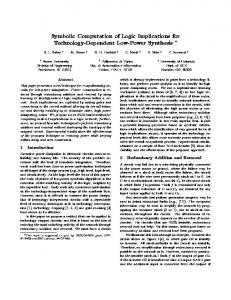
To illustrate the potential applications of the methodology in a design flow for embedded systems, we propose a couple of simple but explanatory use cases. The results shown below have been obtained with a prototype tool, constructed using the NuSMT model checker along the lines described in the previous sections. In both examples we use a periodic task system S1 = {τ1 , τ2 }. Periods are fixed and chosen equal to the relative deadline: T1 = D1 = 20 and T2 = D2 = 30. Use case 1: For this example, we consider a design scenario in which the computation times are not known with a sufficient precision and the system is very close to the border of the schedulability region found with traditional real-time scheduling theory (i.e., assuming null offset). The design problem is how to choose a positive offset O2 so as to maximize the schedulability region (and hence the robustness of the system). To this end we can compute the schedulability

Region with O2 = 0 Or O2= 10 Region with O2 = 5 Region with O2 = 8

21

3

5

7

9

11

13

15

17

19

21

Figure 6. Feasibility regions in the domain of C1 and C2 for different values of O2 region with respect to the following set of free parameters: {C1 , C2 , O2 } fixing O1 = 0. The tool, after some iteration, produces the following symbolic expression for the feasibility region: (C1 < 20) (C1 + C2 < 30) (C1 + C2 < 20 (2C1 + C2 < 40 (C2 < 20 − O2 (C1 + C2 < 20 (C1 + C2 < 20

∨ ∨ ∨ ∨ ∨

2C1 + C2 < 30 + O2 ) 3C1 + C2 < 50) C1 + C2 < 40 − O2 3C1 + 2C2 < 60 2C1 + C2 < 30)

∨ ∨

2C1 + C2 < 30) 4C1 + 2C2 < 60 + O2 )

In Fig. 6, we can see three different sections obtained cutting the three-dimensional schedulability regions with the planes O2 = 0, O2 = 5, and O2 = 8. In accordance with the findings of real-time scheduling theory, O2 = 0 corresponds to the smallest schedulability region. The choice O2 = 8 is the one that ensures the maximum robustness for the choice of C1 , while O2 corresponds to the greatest schedulability region. Use case 2: In the next example, we consider that the worst computation time of the tasks are fixed, C1 = 11 and C2 = 12. This task system is not schedulable with zero offsets as it is possible to see with a standard response time analysis. Therefore, our purpose is to identify the possible values for the offsets O1 and O2 that make the system schedulable. Using the tool, we computed the feasibility region, in the domain O1 × O2 , expressed in the constraints below: (O2 < O1 + 7 ∨ O2 > O1 + 4)∧ (O2 < O1 − 3 ∨ O2 > O1 − 6)∧ (O2 < O1 + 17 ∨ O2 > O1 + 14)∧ (O2 < O1 − 13 ∨ O2 > O1 − 16)∧ ...

The feasibility region for this case is not even connected, as it consists of parallel stripes as shown in Fig. 7. This is a perfectly natural result since by increasing the offsets, we periodically get the same system (except for an initial transient). Therefore, the procedure can converge only because we pose bounds for the search in the parameter space (0 ≤ O1 ≤ 17, 0 ≤ O2 ≤ 20). 87

Authorized licensed use limited to: UNIVERSITA TRENTO. Downloaded on April 28, 2009 at 08:51 from IEEE Xplore. Restrictions apply.

∧ ∧ ∧ ∧ ∧ ∧

19 17 15 13 11 9 7 5 3 1 1

3

5

7

9

11

13

15

17

Figure 7. Regions of feasibility in the domain of O1 and O2. Using those constraints we can simply pick the values for O1 , O2 and O3 inside the feasibility region to make S2 schedulable. We can choose O1 = 5 and O2 = 1 for example. And the system will now be schedulable with the system utility 95%.

7

Related work

A good part of the research on real-time systems has focused on mathematical conditions, whereby a periodic task set scheduled with a fixed priority is schedulable. In their seminal work [21], Liu and Layland identified Rate Monotonic (RM) as the optimal priority assignment to achieve schedulability, and for this assignment they discovered a notorious sufficient schedulability condition on the total CPU utilization of the tasks. Albeit very important, this test fails to provide a conclusive response on the system schedulability in many cases of practical and theoretical interest. Pandya and Joseph [18] proposed an alternative approach. Their methodology allows one to compute the response time of each task, and hence conclude schedulability by comparing it with the deadline. The authors still assume periodic activations for the tasks, but they do not pose restrictions on the priority assignment and on the position of the deadlines. The methodology produces the exact response time if the tasks do not have an initial offset and an overapproximation if the tasks have offsets. Extensions exist for periodic tasks with offsets [25] but they are either intractable or produce conservative results. This analysis techniques have been generalised in different directions. For instance, using the results in [26], it is possible to consider tasks sharing resources. Our approach differs from the ones in the papers cited above since the proposed SATA techniqe performs an exaustive analyisis for much more general activation patterns without making conservative approximations. This tech-

nique lies in the track opened by Wang Yi and his coworkers, who reformulate the problem of schedulability analysis as one of reachability for a network of timed automata. The first attempt in this direction can be found in [24], where the authors use the technology in the UPPAL tool [3] to analyse the schedulability of a set of tasks assuming a non-preemptive policy. This approach of solving the schedulability analysis through reachability problem is also used in [16]. The transition from non-preemptive to preemptive scheduling was not obvious, since many authors used a class of automata for modeling the system (the stop watch automata) [23, 12, 8], for which the reachability problem is known to be undecidable. In [15], the authors proposed a different model for the system based on an extension of timed automata, for which the reachability problem is decidable. In [14], the authors identify an efficient encoding for the schedulability problem in the special but important case of a fixed priority scheduler. In our paper, we generalised this model allowing for parametric constraints associated to the guards and to the invariant conditions of the timed automata. Parametric timed automata can be found in some previous work, but to the best of our knowledge our work is the fist attempt to use this formalism, combined with symbolic computation, to identify the schedulability region. In [28], the authors present a method to model check a real time system using parametric timed automata when a constraint over the parameter is given. This problem is referred to as the “emptiness” problem for PTA and has been prove undecidable, in the general case, in [2]. Interestingly, in [17] a subclass of PTA called L/U PTA is identified for which the problem is decidable, and a solution strategy based on Parametric Difference Bound Matrices is proposed. The solution to the emptiness problem is actually used in this paper as a step to solve a more general problem: producing the region of parameters for which the system is unschedulable (namely, the subroutine named PTA.reachable(Error) in Fig. 3). We have provided theoretical evidence that for periodic task sets the algorithm terminates (and hence the problem is decidable). Further investigation on more general examples, along the lines shown in [17], is reserved for future work. The problem of finding the feasibility region was attacked in analytic terms in [5]. The authors considered periodic task sets and improve a methodology, first introduced by Lehoczky and Sha [19], to identify the minimal representation for the region of feasible computation times. This approach is applicable to strictly periodic task sets with zero offsets. As recalled above, we consider much more general activation patterns, although, as a first step, we offer strong convergence results only for the case of periodic task sets with free offsets.

88

Authorized licensed use limited to: UNIVERSITA TRENTO. Downloaded on April 28, 2009 at 08:51 from IEEE Xplore. Restrictions apply.

8

Conclusions

[11] A. Cimatti, A. Griggio, and R. Sebastiani. Efficient interpolant generation in satisfiability modulo theories. In TACAS’08, volume 4963 of LNCS, pages 397–412. Springer, 2008. [12] J. C. Corbett. Modeling and analysis of real-time ada tasking programs. In RTSS’94, pages 132–141, 1994. [13] M. W. Dawande and J. N. Hooker. Inference-based sensitivity analysis for mixed integer/linear programming. Oper. Res., 48(4):623–634, 2000. [14] E. Fersman, L. Mokrushin, P. Pettersson, and W. Yi. Schedulability analysis using two clocks. In TACAS’03, volume 2619 of LNCS, pages 224–239. Springer, 2003. [15] E. Fersman, P. Pettersson, and W. Yi. Timed automata with asynchronous processes: Schedulability and decidability. In TACAS’02, pages 67–82, London, UK, 2002. SpringerVerlag. [16] A. Fredette and R. Cleaveland. Rtsl: a language for realtime schedulability analysis. In RTSS’93, pages 274–283, Washington, DC, USA, 1993. IEEE Computer Society. [17] T. Hune, J. Romijn, M. Stoelinga, and F. W. Vaandrager. Linear parametric model checking of timed automata. In TACAS’01, pages 189–203, London, UK, 2001. SpringerVerlag. [18] M. Joseph and P. K. Pandya. Finding response times in a real-time system. The Computer Journal, 29(5):390–395, 1986. [19] J. P. Lehoczky, L. Sha, and Y. Ding. The rate-monotonic scheduling algorithm: Exact characterization and average case behavior. In RTSS’89, pages 166–172, 1989. [20] J. Y.-T. Leung and M. L. Merrill. A note on preemptive scheduling of periodic, real-time tasks. Inf. Process. Lett., 11(3):115–118, 1980. [21] C. L. Liu and J. W. Layland. Scheduling algorithms for multiprogramming in a hard-real-time environment. J. ACM, 20(1):46–61, 1973. [22] C. Lu, J. A. Stankovic, T. F. Abdelzaher, G. Tao, S. H. Son, and M. Marley. Performance specifications and metrics for adaptive real-time systems. RTSS’00, 00:13, 2000. [23] J. McManis and P. Varaiya. Suspension automata: A decidable class of hybrid automata. In CAV’94, pages 105–117, London, UK, 1994. Springer-Verlag. [24] C. Norstr¨om, A. Wall, and W. Yi. Timed automata as task models for event-driven systems. In RTCSA’99, page 182, Washington, DC, USA, 1999. IEEE Computer Society. [25] J. C. Palencia and M. G. Harbour. Schedulability analysis for tasks with static and dynamic offsets. In RTSS’98, page 26, Washington, DC, USA, 1998. IEEE Computer Society. [26] L. Sha, R. Rajkumar, and J. P. Lehoczky. Priority inheritance protocols: An approach to real-time synchronization. IEEE Trans. Comput., 39(9):1175–1185, 1990. [27] M. Sheeran, S. Singh, and G. St˚almarck. Checking safety properties using induction and a sat-solver. In FMCAD’00, pages 108–125, London, UK, 2000. Springer-Verlag. [28] D. Zhang and R. Cleaveland. Fast on-the-fly parametric realtime model checking. In RTSS’05, pages 157–166, Washington, DC, USA, 2005. IEEE Computer Society.

In this paper, we presented a general methodology for the symbolic computation of the schedulability region. The methodology applies to very general activation patterns and it does not make any conservative approximations, and is implemented by integrating traditional symbolic model checking and SMT solvers. We proved convergence in the important case of fixed priority scheduling for periodic task systems. For the future, we plan several extensions. First, we aim at the development of a full-fledged design tool implementing the methodology described in this paper. In particular, we plan to optimize the implementation to enable scalability of our solution, and to experiment with different algorithms for the detection of the constraints. On the theoretical side, our most important goal is to extend the study of convergence to the general case. Another interesting possibility, in the spirit of the examples shown in Section 6, is to use the schedulability region as a design tool by introducing appropriate cost functions.

References [1] R. Alur and D. L. Dill. A theory of timed automata. Theor. Comput. Sci., 126(2):183–235, 1994. [2] R. Alur, T. A. Henzinger, and M. Y. Vardi. Parametric realtime reasoning. In STOC’93, pages 592–601, New York, NY, USA, 1993. ACM. [3] T. Amnell, E. Fersman, L. Mokrushin, P. Pettersson, and W. Yi. Times - a tool for modelling and implementation of embedded systems. In TACAS’02, pages 460–464, London, UK, 2002. Springer-Verlag. [4] G. Audemard, A. Cimatti, A. Kornilowicz, and R. Sebastiani. Bounded model checking for timed systems. In FORTE’02, pages 243–259, London, UK, 2002. SpringerVerlag. [5] E. Bini and G. C. Buttazzo. Schedulability analysis of periodic fixed priority systems. IEEE Trans. Comput., 53(11):1462–1473, 2004. [6] R. Bruttomesso, A. Cimatti, A. Franz´en, A. Griggio, and R. Sebastiani. The MathSAT 4 SMT Solver. In CAV’08, LNCS, Princeton, USA, 2008. Springer. [7] G. C. Buttazzo. Hard Real-Time Computing Systems: Predictable Scheduling Algorithms and Applications. Kluwer Academic Publishers, Norwell, MA, USA, 1997. [8] F. Cassez and F. Laroussinie. Model-checking for hybrid systems by quotienting and constraints solving. In CAV’00, pages 373–388, London, UK, 2000. Springer-Verlag. [9] R. Cavada, A. Cimatti, A. Franz´en, K. Kalyanasundaram, M. Roveri, and R. K. Shyamasundar. Computing Predicate Abstractions by Integrating BDDs and SMT Solvers. In FMCAD’07, pages 69–76, Washington, DC, USA, 2007. IEEE Computer Society. [10] A. Cimatti, E. M. Clarke, F. Giunchiglia, and M. Roveri. Nusmv: A new symbolic model verifier. In CAV’99, pages 495–499, London, UK, 1999. Springer-Verlag.

89

Authorized licensed use limited to: UNIVERSITA TRENTO. Downloaded on April 28, 2009 at 08:51 from IEEE Xplore. Restrictions apply.