symbolic computation tuning method for the

U.P.B. Sci. Bull., Series C, Vol. 71, Iss. 4, 2009

ISSN 1454-234x

SYMBOLIC COMPUTATION TUNING METHOD FOR THE EVALUATION OF ALGORITHMS IN SMALL SIGNAL PARAMETERS EXTRACTION Cristian ZORIO1, Mircea BODEA2, Ioan RUSU3 Problema matematică asociată problemei de extracţie a parametrilor unui circuit se reduce la determinarea minimului global al unei funcţii obiectiv obţinută prin metoda celor mai mici pătrate. În cazul analizei de semnal mic a unui circuit (când se utilizează un model liniar), funcţia asociată circuitului este o funcţie raţională, şi în consecinţă şi funcţia obiectiv are aceeaşi formă. Aceasta permite a se lua în considerare rezolvarea sistemului de ecuaţii format cu derivatele parţiale ale funcţiei obiectiv pentru determinarea, în final, a minimului global, metoda care, spre deosebire de metoda pur numerică, nu mai necesită valori “de start” ale parametrilor de extras şi în plus garantează faptul ca rezultatul obţinut corespunde minimului global. Această abordare conduce la problema matematică a rezolvării unui sistem de ecuaţii format cu funcţii raţionale, care poate fi transformat într-un sistem polinomial echivalent. În lucrare se determină modul în care numărul de valori măsurate ale unei funcţii de semnal mic (asociată unui circuit liniar), care se iau în considerare, influenţează gradul acestui sistem iniţial de ecuaţii polinomiale. Se arată faptul că timpul de calcul total, (care depinde de gradul sistemului iniţial de ecuaţii polinomiale şi, de asemenea, de algoritmul de reducere a sistemului polinomial la un sistem echivalent quasi triangular, rezolvabil prin metode numerice) poate fi controlat prin ajustarea acestui număr. Utilizând această proprietate/dependenţă, care permite generarea de probleme matematice (sisteme de ecuaţii polinomiale iniţiale) de complexităţi diferite, pentru aceeaşi problemă de extracţie, se analizează în cazul unui circuit particular, posibilitatea obţinerii unui rezultat într-un timp rezonabil, cu algoritmii incluşi în două sisteme CAD pentru matematică. Concluziile identifică oportunitatea utilizării fiecăruia dintre aceste instrumente matematice, pentru implementarea unui program de extracţie nu neapărat bazat pe un sistem CAD. The math problem associated to the problem of parameter extraction of a circuit can be reduced to the problem of finding the global minimum of an error function obtained with the least squares method. In the case of the small signal analysis of a circuit (when a linear model is considered), the circuit’s associated function is a rational function and as a consequence the error function is of the same form too. This makes possible to take into account solving the resulting 1

Eng., Dept. of IT & Computers, Romanian National Television Society, Bucharest, Romania, [email protected] 2 Prof., Dept. of Devices, Circuits and Electronic Apparatus, University POLITEHNICA of Bucharest, Romania, [email protected] 3 Prof., Dept. of Electronic Technology and Reliability, University POLITEHNICA of Bucharest, Romania, [email protected]

64

Cristian Zorio, Mircea Bodea, Ioan Rusu

equation system, formed with the partial derivatives of the error function, in order to find, in the end, the global minimum of the error function. The method, unlike any pure numeric method, no longer requires "start” values for the parameters being extracted and also guarantees that the final result corresponds to the global minimum. This approach leads to the mathematical problem of finding the solutions of an equation system formed with rational functions, which can be transformed in an equivalent polynomial system. The paper highlights the dependency of the degree of this initial polynomial equation system, with the number of measured values of a linear circuit small signal function which is considered in a particular extraction problem. It is shown that the total execution time (which depends on the degree of the initial polynomial system and also on the algorithm for reducing the system to an equivalent quasi-triangular, numerically solvable form) can be “tuned” by adjusting this number. Using this property/dependency which makes possible to generate several mathematical problems (initial polynomial equation systems) having different complexities, for the same extraction problem, we analyze, using a particular circuit, the possibility of getting a solution in a reasonable amount of time, with the algorithms implemented in two different Math-CAD systems. The conclusions identify which of the mathematical instruments used, could be used to implement a standalone program for extraction, which should not necessarily be based on a CAD system.

Keywords: symbolic analysis, modified nodal analysis, small signal analysis, parameter extraction, SPICE input format 1. Introduction Extraction of the parameters of a circuit generally leads to the mathematical problem of finding the global minimum of an error function which is determined by the mathematical model of the circuit and the measured values of some circuit signals. A classical approach for solving the parameter extraction problem (finding the input values of the error function, corresponding to the function’s global minimum) is by using a numerical method for generating a convergent descendent sequence of error function values. This method is based on an algorithm which evaluates the function and selects for the current input values those that reduce the gap between calculated and evaluated values, leading to a minimum of the error function. The algorithm stops when all possible modifications of the parameters representing input values for the error function could not further reduce the value of the error function. This approach is basically a numeric “refinement” process and although it always leads to some minimum of the error function, it can not guarantee that the sequence of errors converge to the global minimum of the function (and not to some different local minimum). The result of the convergence process depends on an initial set of parameter values (the “start values”) representing the iteration starting point. The appropriate “guess method” for obtaining these values is by

Symbolic computation tuning method for the evaluation of algorithms in small signal param. 65

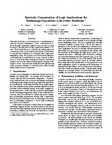
using the engineer’s intuition based on practical experience and/or by using an alternative simplified, easy to compute, model of the circuit to estimate somehow the (approximate) values of the parameters to be extracted. However, any user applying this method, could not invoke conclusive rigorous arguments which might prove that any of the “guessed starting points” will lead through the process of “refinement” to the global minimum of the error function, and not to any of its local minimums. A different approach, not based on numerical pure algorithms using convergence of a sequence of error values, is a symbolic computation method that could potentially find all the minimums of the error function. In theory, this is always possible by computing all the partial derivatives of the error function and solving the resulting equation system. Two minimal conditions are required for this approach: - a symbolic formula of the error function must exist (not only a procedure/algorithm for numerical evaluation) - the equation system formed with partial derivatives has to be solvable using numerical and/or symbolic computation method. An example of parameter extraction in the case of a linear circuit, that use Maple [1] Math-CAD system to perform symbolic calculation of all the minimums of an error function combined with numeric procedures for finding real roots of polynomials of one variable, was already presented in [4]. 2. Mathematical model of the “extraction problem” The generalization of the following example will help us to eliminate the task of giving formal definitions for all the elements of the mathematical model associated with the “parameter extraction problem”. Assume a given circuit having a well determined schema for which some of the values of the circuit elements (discrete devices) are unknown and have to be determined by indirect measurements. Also assume that we dispose of the real circuit which can be subject of different measurements at its input and output gates. 3. Example of a circuit and measurements The circuit of Fig. 1 which has already been subject of symbolic parameter extraction, [4], (when the resultant method for variable elimination was used) will be used again, in the next sections for generating an example of polynomial equation system to be solved with different algorithms. X Example:

66

Cristian Zorio, Mircea Bodea, Ioan Rusu

rμ rb

1

cμ

2

rb

rc

4

rb

rb

5

=

0

rb

rb

rb

io

cπ ro

rπ

V1

ic

Vi

vo= 0

3 rb

re m i

ic = g m v 1 =

v v1 = 1 rm x8

0 rb

Fig. 1 - Circuit Example – The Giacoletto equivalent circuit of a bipolar transistor

Solving the “parameter extraction problem” for the circuit of Fig. 1 when knowing the values of a subset of its elements (see Table 1) means finding the values of the unknown components, rb and gm, by comparing calculated and measured values of some small signal input/transfer/output functions of the circuit. Circuit’s Input/Transfer/Output function Since the circuit’s schema is well determined any small signal input/transfer/output function can be computed as a symbolical expression which contains the schema elements. Considering, for instance, the input impedance z11=z11(gm, rb, rπ , rμ, re, ro , rc , cπ , cμ ,f) of the circuit (which was computed with the nodal method [5] and using a specialized script [3]) leads to (1): z11 =

ii vi

= z in (rb , rπ , rμ , re , ro , g m , cπ , c μ , f ) = Vo = 0

R (rb , rπ , rμ , re , ro , g m ,cπ , c μ , f ) S (rb , rπ , rμ , re , ro , g m ,cπ , c μ , f )

with: R (rb, gm, f)= -rbrore -rbrπrc -rbrµre -rbrπro -rbrµro -rorerµ -rbrµrc -rorerc -rπrorµ -rπrerµ j2πfCπrπrorerc -j2πf Cπrπrerµrc -rbrπre -rπrerc -gmrπrorerc -gmrπrorerµ -rbrπgmrore rbrπrcgmro +4π2f 2CπrπroreCµrµrc +4π2f2CπrbrπrµroCµrc -rπrorc +4π2f 2 CµrbrπrµCπrore -rbrorc -rπrµrc -rerµrc +j(-2πfCπrπrorerµ -2πf rore Cµrµrc -2πf gmrπroreCµrµrc -2πfrπre Cµrµrc -2πf rπro -2πf Cπrbrπrorc -2πf Cπrbrπrµrc -2πf Cπrbrπrµro -2πf rbrµro Cµrµrc -2πf Cπrbrπrµre r -2πf r r r r -2πf -2πf Cµrbrπrµgmrore -2πfCµrbrπrµre Cµ c b π Cπ o e Cµrbrµrore 2πfCµrbrπrµrc -2πfCµrbrπrµro -2πfrbrπrcgmrµroCµ) S (rb, gm, f)= -rµrc -rµro -rπre -rπro -rerµ -rπrc -rorc -rore -gmrπrore -rπrcgmro +4π2f 2CπrπrµroCµrc +4π2f 2CµrπrµCπrore

(1)

Symbolic computation tuning method for the evaluation of algorithms in small signal param. 67

+j(-2πf rπroCµrµ -2πf rπrcgmro Cµrµ -2πf rerµ Cπrπ -2πf Cπrπrµrc -2πfrore Cµrµ 2πfCπrπrµro -2πf gmrπrore Cµrµ -2πf Cπrπrorc -2πf Cµrµrorc -2πf Cπrπrore -2πf rπre Cµrµ -2πf rπrc Cµrµ)

The values for the known elements are given in Table 1 (see the “Initial notation” row): Table 1 Initial notation

gm

rb

rπ

rμ

re

ro

rc

cπ

cμ

Initial notation - numeric indexes

1/r1

r2

r3

r4

r5

r6

r7

c1

c2

Notation using vector elements

x1

x2

x3

x4

x5

x6

x7

x8

x9

Values

−

−

Units

Ω−1

5 × 103 2×108 2 1×105 50 2 × 10−11 Ω

2×10−1 3

F

The known values for rπ , ,rμ , re, ro , rc , cπ , cμ , can be substituted in the symbolic formula, resulting an expression (2) which depends only on the unknown values rb and gm , “to be extracted” and the frequency f. z in (rb , rπ , f ) =

R ( rb , rπ , f ) A( rb , rπ , f ) + jB ( rb , rπ , f ) = S ( rb , rπ ,, f ) C ( rb , rπ , f ) + jD( rb , rπ , f )

with: R (rb, gm, f) = A (rb, gm, f) + jB (rb, gm, f) = = 0.6500000000×1011gmrb+0.5000001250×1018gm−0.2052877716×10−2rbf2+ +0.5001166326×1014rb−0.3947841762×10−2f2+0.2501520825×1018+ +j(31739961.09rbf + 16336281.80gmrbf + 31415926.54gmf + 78558807.28f)

(2)

S (rb, gm, f)= C (rb, gm, f) + jD (rb, gm, f) = = 0.6500000000×1011gm−0.2052877716×10−2f2+0.5001166326×1014+ j (16336281.80gmf + 31739961.09f)

R and S are polynomials having complex (pure real or pure imaginary) coefficients and A, B, C, D, are polynomials having real coefficients (to be approximated by rational number). 4. Error function formula Without loosing in generality, using the example of the particular circuit of Fig. 1 and including also the data of Table 1, an extraction model can defined. In order to illustrate the result’s complexity and size, the huge particular symbolic

68

Cristian Zorio, Mircea Bodea, Ioan Rusu

formula of this circuit’s Error function was already computed, [4], and will not be reproduced here again. The circuit’s function - general case Table 1 also provides a method of renaming the circuit’s elements, which can be easily generalized to any circuit. The elements having unknown values, which must be determined by “extraction”) are in the first columns of the table so that, when using the “x1,...,xN” notation, substituting symbolic names with numerical values should always replace the last xk,...,xN , k>1, symbols with their corresponding values having the effect of reducing N. The general “x1,...,xN” notation, will be used next, for an input/transfer/output function associated to any circuit so that the left part of the expressions (1) or (2) can be rewritten as: ψ = ψ ( g m , rb , rπ , rμ , re , ro , c1 , c 2 , f ) = ψ ( x1 ,..., x N , f ) (3) with N=8 when rewriting (1) or N=2 when rewriting (2). When dealing with linear circuits, expression (1) or (2) can be regarded as rational functions, as a particular form of a general expression (3). Also, in the linear case, the numeric values replacing symbolic elements xi, are embedded in the coefficients of the resulting rational functions (see §0). The following general definitions for “distance” and “global error function” do not necessarily restrict ψ=ψ(x1,…, xN, f), the function associated to a linear circuit, to be a rational function. Distance formula Since we dispose of measurements results for the values of the circuit’s associated function, and since we can also compute such values by evaluating its formula for different values of the parameters (the schema elements with undetermined values), it make sense to define a “distance” d=d (ψCal, ψm), between “measured” values, ψm, and “calculated” values ψCal (4): dm = d(ψ mCal,ψ m ) = {Re [ψ (x1 ,...,xN , f m )]− Reψ m }2 +{Im ψ (x1 ,...,xN , f m )]− Imψ m}2

(4)

Note that each “distance” dm=d (ψmCal, ψm) depends of the frequency values fm chosen for each measurement of ψm (“the good complex value” for ψ). Error function formula (global distance) The general method for parameter extraction uses an error function that estimates a “global” distance” (5), (6): M

M

m=0

m=0

E(x1,...,xN ) = ∑dm = ∑d[(x1,...,xN , fm),ψm]

2

(5)

Symbolic computation tuning method for the evaluation of algorithms in small signal param. 69

E ( x 1 ,..., x N ) =

M

∑ {[Re ψ ( x m =1

1

,..., x N , f m ) − Re( ψ m )] 2 +

(6)

+ [Im ψ ( x 1 ,..., x N , f m ) − Im( ψ m )] 2 }

The values xo1 , ... ,xoN which put the error function in its global minimum, represent the values which give an optimal fit of the circuit’s calculated values (using ψ‘s formula) with the measured values, and represent “extracted parameters”. This approach leads to the mathematical problem of finding the global minimum of a function, having a more or less complex formula. The case of a linear circuit In the case of a small signal linear circuit the input/transfer/output function ψ=ψ(x1,…, xN, f), which represents the behavior of the circuit, has of the form of a rational function, [5]: ψ = ψ ( x1 ,..., x n , f ) =

R ( x1 ,..., x n , f ) A( x1 ,..., x n , f ) + jB ( x1 ,..., x n , f ) = S ( x1 ,..., x n , f ) C ( x1 ,..., x n , f ) + jD( x1 ,..., x n , f )

(7)

where R and S are polynomials with real or pure imaginary coefficients, and A, B, C, D are polynomials with real coefficients such as: R ( x1,..., xn , f ) = A( x1,..., xn , f ) + jB( x1,..., xn , f ) and S ( x1,..., xn , f ) = = C ( x1,..., xn , f ) + jD( x1,..., xn , f )

(8)

This was the case of expressions (1) and (2) for zin=z11(gm, rπ , ,rμ , re, ro , rc , cπ , cμ ,f). As a consequence the error function will be a rational function with real coefficients, (9): E ( x 1 ,..., x N ) = =

2 2 ⎧⎪ ⎡ ⎛ R ( x ,... , x , f ) ⎞ ⎤ ⎡ ⎛ R ( x 1 , ... , x n , f m ) ⎞ ⎤ ⎫⎪ n m 1 − + − Re Re( ψ ) Im Im( ψ ) ⎜ ⎟ ⎜ ⎟ ⎨⎢ ∑ m ⎥ m ⎥ ⎬ ⎢ ⎝ S ( x 1 , ... , x n , f m ) ⎠ m =1 ⎪ ⎣ ⎦ ⎣ ⎝ S ( x 1 ,... , x n , f m ) ⎠ ⎦ ⎪⎭ ⎩ M

(9)

which can be rewritten as (10) , if taking into account the notations (8): E ( x 1 ,..., x N ) = 2 ⎧ ⎡ A ( x , ... , x , f ) C ( x ,... , x , f ) − B ( x ,... , x , f ) D ( x ,... , x , f ) ⎤ ⎪ 1 1 1 1 n m n m n m n m − rm ⎥ + = ∑ ⎨⎢ [C ( x 1 ,... , x n , f m ) ]2 + [D ( x 1 ,... , x n , f m ) ]2 m =1 ⎪ ⎣ ⎥⎦ ⎩⎢ M

2 ⎡ A ( x 1 , ... , x n , f m ) D ( x 1 ,... , x n , f m ) − B ( x 1 ,... , x n , f m ) C ( x 1 , ... , x n , f m ) ⎤ ⎫⎪ +⎢ − xm ⎥ ⎬ [C ( x 1 ,... , x n , f m ) ]2 + [D ( x 1 ,... , x n , f m ) ]2 ⎥⎦ ⎪⎭ ⎣⎢

(10)

70

Cristian Zorio, Mircea Bodea, Ioan Rusu

where: (11) Notice that in the case of a linear circuit, a symbolic formula of the error function can always be determined and the process of calculating a function value with the formula for known input values means evaluation of this formula. rm=Re(ψm) , x= xm=Im(ψm)

5. Analysis of intermediate symbolic expressions complexity when computing a polynomial system from a system of rational functions Initial system of polynomial equations A straight forward method for determining a global minimum of the error function Ε=E(x1 , ... , xN), is to choose the smallest point of extremis of Ε, after determining all the point of extremis. We will assume that Ε has a finite set of points of extremis, as a consequence of physical interpretation of the significance of global Error function Ε. Interpretation of the algebra theory concerning “the dimension of an affine variety” [7] should lead to the same conclusion. Since we dispose of the symbolic expression, (9), (10), of the Error function Ε=E(x , ... , xN), a first step in this direction is calculating the symbolic expressions of its partial derivatives, and constructing the system : ∂E ( x1 ,..., x n ) = 0 ; i = 1...N ∂ xi

(12)

This is a system of rational functions which can be transformed into a system of polynomial equations and solved with modern algebra theory [7]. Solving polynomial equation systems using common algebraic methods, is always possible if considering infinite computing resources and/or an infinite computing time [7], but when taking into account the possibility of obtaining practical results, the complexity of the initial equation system and of the solving algorithms must be considered too. This introduces the necessity of a more precise definition for the notion of “complexity” of the input data of these algorithms i.e. the “complexity” of some given initial polynomial equation system which is to be solved. The quantifiable properties of any specific initial polynomial equation system, used to measure its complexity, s, n, d, h, are variables on which the formulae used to calculate the complexity of a solving algorithms depends on, [9]: s is the number of equations, n is the number of variables (in our case s=n), d is total degree (associated with a given monomial ordering [7] and referred next as “total degree”), and h (height) representing the number of bits needed to store denominator/numerator of each rational numbers representing polynomial coefficients.

Symbolic computation tuning method for the evaluation of algorithms in small signal param. 71

Since h affects “numeric precision” which at least at this stage, can be considered, a refinement feature, and any analysis concerning s or n, the number of equations/variables, is obvious and straightforward, the next paragraphs will focus on the order of magnitude of the “total degree” n of the equation system of rational functions (12) and simplifying it’s symbolic formula. Symbolic transformations and influence of the applying order The left part of each of the equations of system (12) can be regarded as a symbolic formula, (15) which has to be transformed in a sum of rational functions having each the same denominator, which could be then eliminated, so that only the numerators of each sum/equation should form a polynomial equation system. The set of solutions of this polynomial system will always include the solutions of the initial system (12). Main computations for transforming symbolic formulae into equivalent formulae The main symbolic computations (operators) used to modify symbolic formulae, for the above mentioned purpose, into equivalent expressions are: • Real and Imaginary part calculus/separation • Adding/subtracting measured values to/from rational expression (13) • Calculating squares in each term • Partial derivative symbolic calculus • Calculating a common denominator for all terms and summing The result of any of these symbolic transformations is always a rational function and each possible transformation have as input (see (15), (16) ) symbolic formulae of the type of a rational function or a sum of rational functions including complex constants (measured) values. The input selected operand of each “main computation” depends on the selected order for applying the operands (like exemplified next for the derivation operator in section §0). The total effect of these operations on the degree of intermediate polynomials (presented in section §0, after selecting an order of applying these main transformations too) will give the complexity (i.e. degree) of the final polynomial system. Simplifying symbolic computations The symbolic formulae (rational functions) representing partial results of the main transformation process of symbolic formulae may be the subject

72

Cristian Zorio, Mircea Bodea, Ioan Rusu

simplifying operations before making further (main) transformations by the rest of the above main transforming operations(13), in order to keep numerators and denominators of rational functions as simple as possible. Possible simplification operations are: o Elimination of common factors between numerator and denominator of each term o Factorizing numerators after derivation o Finding a greatest common multiple between all denominators for the simplest common denominator (14) before summing o Choosing a set f1,…,fM for factorizing [C (x1 , ... , xN , fm)]2 + [D (x1 , ... , xN , fm)]2 The simplification operations (14) that can be used after each main operation (13) are presented in section §0. Influence of the order of symbolic computations A selection for the order in which main operations are applied can be considered to be well defined after stating one of the equivalent forms of the math formula (15) (i.e. like formula (16)) representing the left term of equations (12). The computing power of modern Math-CAD like Maple, [1], or Singular, [2], makes possible to find a final formula of each derivative ∂ E ∂ x i independently of the order of applying the main operators (13). However, choosing the best order simplifies insight on partial results and can evidence the fact that some intermediate symbolic formula of the error function could have simpler intermediate expression. An appropriate selection of the order of applying the main operators (13) permits an earlier use of any of the appropriate simplifying operations (14), providing smaller intermediate formulae representing simpler operands for the next main operator (13). As an example, take into account computing the symbolic derivates of Ε=E(x1 , ... , xN), starting from expression (6) where we substitute ψ=ψ (x1, ... ,xN , fm) with its rational expression (7). Partial derivation can be done after applying all other transformations (15): ∂ E ( x 1 ,..., x N ) = ∂x i =

∂ ∂x i

2 2 ⎧⎪ ⎡ ⎛ R ( x ,... , x , f ) ⎞ ⎤ ⎡ ⎛ R ( x 1 , ... , x n , f m ) ⎞ ⎤ ⎫⎪ (15) 1 n m − + − ψ Im( ψ ) Re( ) Im Re ⎜ ⎟ ⎜ ⎟ ⎨⎢ ∑ m ⎥ m ⎥ ⎬ ⎢ ⎝ S ( x 1 , ... , x n , f m ) ⎠ m =1 ⎪ ⎣ ⎦ ⎣ ⎝ S ( x 1 ,... , x n , f m ) ⎠ ⎦ ⎪⎭ ⎩ M

Symbolic computation tuning method for the evaluation of algorithms in small signal param. 73

or, the derivation operator can be “distributed” the derivation operator to each term of the sum: ∂E( x1,...,xN ) = ∂xi 2 2 ⎧⎪ ∂ ⎡⎛ ⎛ R( x ,..., x , f ) ⎞ ⎞ ⎛ ⎛ R( x1,..., xn, fm ) ⎞ ⎞ ⎤⎫⎪ n m 1 = ∑⎨ ⎢⎜⎜ Re⎜ ⎟ − Re(ψ m ) ⎟⎟ + ⎜⎜ Im⎜ ⎟ − Im(ψ m ) ⎟⎟ ⎥⎬ S ( x1,..., xn , fm ) ⎠ m=1 ⎪ ∂xi ⎢⎝ ⎠ ⎝ ⎝ S ( x1,..., xn , fm ) ⎠ ⎠ ⎥⎦⎪⎭ ⎩ ⎣ ⎝ M

(16)

In both (15) and (16) cases, the function to which the derivation operator applies is a rational function and the consequence of derivation to degrees of the numerator and denominator could be the same in terms of final degree, as presented next, in section §0, so it seems that the “moment” of using ∂ ∂ x i does not matter. On the other hand applying the derivation operator on each term of the sum, like in (16) i.e. before considering multiplying the denominator and numerator of each term of the sum (15) by some polynomials (in order to generate a common denominator for each term) could lead to numerators of terms which have a common factor. This factor could be separated as a common multiplier of each term before doing the symbolic calculus of the sum. As a consequence, formula (16) gives a better order selection for the derivation calculation than (15). Effect of symbolic computations on total degree Degrees of the denominator and numerator polynomials after each transformation are always substantially bigger than the ones of the rational function that represented the (whole or partial) input of the symbolic transformation operator. This section analyzes the effect on the degree of intermediate formulae of the main, (13) and simplifying, (14), operations, and also defines the selected order for the main operations (which must be applied from the “inside” to the “outside” of relation (16) ). • Real and Imaginary part calculus/separation Separation of the Real and Imaginary parts of the circuit function which is included in each term, results in (17):

( A m + jB m )(C m − jD m ) R ( x 1 ,... , x n , f m ) A + jB m = = = m S ( x 1 ,... , x n , f m ) C m + jD m (C m + jD m )(C m − jD m )

=

Am C m − B m D m

(C m )2 + (D m )2

− j

Am D m − B m C m

(17)

(C m )2 + (D m )2

where Am=A(x1 , ... ,xN, fm), Bm=B(x1 , ... ,xN, fm) respectively Cm=C(x1 , ... ,xN, fm), Dm=D(x1 , ... ,xN, fm) are polynomials with real coefficients representing the real

74

Cristian Zorio, Mircea Bodea, Ioan Rusu

and imaginary parts of Rm=R(x1 , ... ,xN, fm), the numerator respectively Sm=S(x1 , ... ,xN, fm) the denominator of the circuit’s function evaluated at fm ,(18): Re[R( x1 ,..., x n , f m ) ] = Am = A( x1 ,..., x n , f m ) = Am ( x1 ,..., x n ), Im[R( x1 ,..., x n , f m ) ] = Bm = B( x1 ,..., x n , f ) = Bm ( x1 ,..., x n ), (18) Re[S ( x1 ,..., x n , f m ) ] = C m = C ( x1 ,..., x n , f m ) = C m ( x1 ,..., x n ), Im[S ( x1 ,..., x n , f m ) ] = Dm = D( x1 ,..., x n , f ) = D m ( x1 ,..., x n ) Relations (17) and (18) show that, before derivation, the final degree of the two denominators of each term in the sum (15) become the double of the maximum degree of the denominator’s and numerator’s real and imaginary part,(19): deg((Cm) 2+( Dm)2)= 2· max{ deg(Cm), deg[Dm)} (19) For the numerator of the real and imaginary parts, the new degrees are, (20): deg(Am Cm + Bm Dm) = max{ deg(Am)+ deg(Cm) , deg(Bm)+ deg(Dm) } (20) and respectively (21) for the imaginary part: deg(Am Dm + Bm Cm) = max{ deg(Am)+ deg(Dm) , deg(Bm)+ deg(Cm)} (21) • Adding/subtracting measured values to/from rational expression Including the measured values rm=Re(ψm) and respectively xm=Im(ψm) in the rational expression of each term (22) respectively (23), does not affect the degree of the (same) denominator of each rational function’s term representing a real or imaginary part: A C − Bm Dm ⎛ R( x1,..., xn , f m ) ⎞ Re⎜ −r = ⎟ − Re(ψ m ) = m m2 ( ... ) S x , , x , f [Cm ] + [Dm ]2 m 1 n m ⎠ ⎝

[

]

A C − Bm Dm − (Cm ) + (Dm ) rm Pm = m m = 2 2 2 (Cm ) + (Dm ) (Cm ) + (Dm )2 2

2 2

A D − BmCm ⎛ R( x1,..., xn , fm ) ⎞ Im⎜ −x = ⎟ − Im(ψ m ) = m m2 ( ... ) S x , , x , f (Cm ) + (Dm )2 m 1 n m ⎠ ⎝

[

]

A D − BmCm − (Cm ) + (Dm ) xm Qm = m m = 2 2 2 (Cm ) + (Dm ) (Cm ) + (Dm )2 2

2

(22)

(23)

Relations (22) (23) show that the degree of the numerator in each term, corresponding to the real/imaginary parts, becomes the maximum of the numerator’s and denominator’s degree of the previous symbolic operation. X Note:

Symbolic computation tuning method for the evaluation of algorithms in small signal param. 75

Since the chosen frequency values fm and respectively the measured numeric values rm, and xm for the complex impedance, will be embedded in the three different polynomials representing numerators or denominators of the resulting rational functions calculated with the relations (22) and (23), each of these polynomials will respectively have the same monomials and different coefficients for each m. X Note: An important observation which can be made at this point and resulting from the relations (22) and (23), is that the fm values, will be embedded each, in the coefficients numeric values of the numerator and of the denominator polynomial of each term, while the measured values rm respective xm, will be included only in the calculation of the numeric coefficients of each “real” (22) and respective “imaginary” (23) numerators polynomials, in each term. o Choosing a set f1,…,fM for factorizing [C (x1 , ... , xN , fm)]2 + [D (x1 , ... , xN , fm)]2 X Note: In a later stage of the symbolic calculation, after analyzing the effect of multiplying for each m the term’s numerator and denominator with the same polynomial, in order to obtain a common denominator for all the terms before computing the sum, the property of independence of the numerator’s coefficients of rm respective xm, could be used in a symbolic simplifying computation which could find a simpler common denominator. •

Calculating the square in each term and summing the two numerators of one term Each term Tm of the left part of any equation is, (24): ⎤ ⎡ ⎤ ⎡ (Pm )2 + (Qm )2 Pm Qm Tm = ⎢ = + ⎢ 2 2 2⎥ 2 2 ⎥ (Cm )2 + (Dm ) ⎣⎢ (C m ) + (Dm ) ⎦⎥ ⎣⎢ (C m ) + (Dm ) ⎦⎥ 2

2

[

]

(24)

The denominator’s coefficients still does not depend on rm and xm, and it’s final denominator (25) is four times of the maximum of the initial real and imaginary parts of the circuit’s function denominator: deg([(Cm) 2+( Dm)2]2)= 2· max{ deg([Cm]2), deg([Dm]2)}= 4· max[ deg(Cm), deg(Dm)] (25) The numerator’s degree increases with a factor of 2 the maximum of the former two numerators corresponding to the real and imaginary part of the circuit’s function, because, (26): deg([Pm] 2+[ Qm]2)= max{ deg([Pm]2), deg([Qm]2 ) }= 2· max{ deg(Pm), deg(Qm)} (26) X Note:

76

Cristian Zorio, Mircea Bodea, Ioan Rusu

After computing the square of each of the expressions of the resulting rational functions (22) and (23), and summing each term’s numerators, all the next (main or simplifying) symbolic operations applied to each term (before the intermediate symbolic expression allows performing the sum itself) will preserve the following property of the terms: each term is a rational functions with the same monomials but different numeric coefficients depending only of the fm’s values for the denominators and of the fm’s values but also of the rm’s and xm’s for the numerators. • Calculating partial derivatives Taking into account (27) and (28) for partial derivation: 2

⎤ ∂ ⎡ ⎛ R ( x1, ... , xn , f m ) ⎞ Re ⎜ ⎟ − Re(ψ m ) ⎥ = ∂xi ⎢⎣ ⎝ S ( x1, ... , xn , f m ) ⎠ ⎦

[(C

2

Pm ∂ = ∂xi (C m )2 + (Dm )2

[

∂ ∂ xi

]

2

)2 + (Dm )2 ]

2

m

=

[

∂ 2 2 ∂ Pm + Pm C 2 + D2 ∂ xi ∂ xi

[(C

[(C

)2 + (Dm )2 ]

2

m

=

)2 + (Dm )2 ]

2

[

[

∂ (Qm )2 + (Qm )2 ∂ (C m )2 + (Dm )2 ∂ xi ∂ xi

[(C

2

4

m

(Qm ) ⎡ ⎛ R ( x1,... , xn , f m ) ⎞ ⎤ ∂ ⎢ Im ⎜ S ( x ,..., x , f ) ⎟ − Im(ψ m ) ⎥ = ∂x 2 2 1 n m ⎠ ⎣ ⎝ ⎦ i (C m ) + ( Dm ) 2

(27)

]

]

]

2

=

(28)

2

)2 + (Dm )2 ]

4

m

the calculus of the derivative of each term gives, (29): ∂ ∂xi

2 2 ⎧⎪⎡ ⎛ R( x ,..., x , f ) ⎞ ⎡ ⎛ R( x1 ,..., x n , f m ) ⎞ ⎤ ⎫⎪ ⎤ n m 1 ⎟ − Im(ψ m )⎥ ⎬ = ⎟ − Re(ψ m )⎥ + ⎢Im⎜ ⎨⎢Re⎜ ⎪⎩⎣ ⎝ S ( x1 ,..., x n , f m ) ⎠ ⎣ ⎝ S ( x1 ,..., x n , f m ) ⎠ ⎦ ⎪⎭ ⎦

[(C ) + (D ) ] ∂∂x P 2 2

2

m

=

m

i

2

+ P2

[

] [

{[C( x ,..., x , f 1

=

]

[

]

4 2 2 ∂ (Cm )2 + (Dm )2 + (Cm )2 + (Dm )2 ∂ Q2 + Q2 ∂ (Cm )2 + (Dm )2 ∂xi ∂xi ∂xi n

m

)] + [D( x1,..., xn , fm )] 2

}

2 4

(29) =

Fi ( x1,..., xN , fm ) [G( x1,..., xN , fm )]4

The degree of each resulting numerators is given by (30): deg(Fi ( x1, … , xN))= max{ deg([Pm]2), deg([Qm]2) }+ deg([(Pm) 2+( Qm)2]2)}-1

(30)

where deg([(Pm) 2+( Qm)2]2) could be replaced using relation (25). In relation (30) subtracting 1 is the consequence of derivation and the addition operation the consequence of multiplying denominator/numerator polynomials or derivative of

Symbolic computation tuning method for the evaluation of algorithms in small signal param. 77

denominator/numerator polynomials with derivative of numerator/denominator or respectively numerator/denominator. The degree of each denominator increases by a factor of 2 and again, the resulting denominator still does not depend on rm and xm. X Note: Since from the partial derivation relation (29), it appears that in each equation i, the derivation operator ∂ ∂ x i does not appear at the denominator of any m-th term, the symbolic expressions of the denominator of the m-th term do not differ ant two equations i. At this point we can consider simplifying the formula of each ∂ E ∂ x i . o Factorizing numerators after derivation If the numerators of all terms of a sum have, after derivation a common factor for the whole sum, this could lead to leaving each term a simpler numerator formula. • Calculating a common denominator for all terms and summing X Note: As a consequence of the fact that the denominator of any m-th term is the same in any two equations i, k, of the system (12), the problem of finding a common denominator for the terms of any equation is unique and the associated symbolic calculation does not depend on the particular equation. In order to effectively calculate a symbolic formula for each sum, one must multiply the denominator and the numerator of each current term with a polynomial that is the less common multiple, LCM, of all the denominators divided by the denominator of the rational function representing the current term (31): ∂E ( x1 ,..., x N ) M Fi ( x1 ,..., x N , f m ) =∑ = 4 ∂xi m=1 [G( x1 ,..., x N , f m )] 4 M ⎡ F ( x ,..., x N , f m ) [LCM ( x1 ,..., x N , f1 ,..., f M ) G( x1 ,..., xn , f M )] ⎤ = ∑⎢ i 1 × = 4 4⎥ m =1 ⎣ ⎢ [G( x1 ,..., x N , f m )] [LCM ( x1 ,..., x N , f1 ,..., f M ) G( x1 ,..., xn , f M )] ⎥⎦

=

M

∑

Fi ( x 1 , ... , x N , f m ) × [LCM ( x 1 , ... , x N , f 1 ,..., f M ) G ( x 1 , ... , x n , f m ) ]

4

[LCM

m =1

=

1

4

(31)

Fi ( x1 ,..., x N , f m ) × [LCM ( x1 ,..., x N , f1 ,..., f M )] G( x1 ,..., xn , f m ) m=1

4

M

[LCM ( x1,..., x N , f1 ,..., f M )]4

=

( x 1 , ... , x N , f 1 ,..., f M ) ]

×∑

with G ( x 1 ,... , x N , f m ) = [C ( x 1 ,... , x N , f m ) ] + [D ( x 1 ,... , x N , f m ) ] 2

2

78

Cristian Zorio, Mircea Bodea, Ioan Rusu

This operation increases the initial degree of each numerator Fi= Fi(x1 , ... ,xN, fm) with the degree of the polynomial LCM(x1 ,..., xN , f1 ,..., fM)/G(x1 , ... ,xN, fm) (32): deg(Fi(x1 , ... ,xN, fm) ×LCM(x1 ,..., xN , f1 ,..., fM)/G(x1 , ... ,xN, fm) )= (32) = deg(Fi(x1 , ... ,xN, fm)+ deg(LCM(x1 ,..., xN , f1 ,..., fM))- deg(G(x1 , ... ,xN, fm)

In the worst case the final common denominator of all terms is the product of all denominators and the polynomial LCM(x1 ,..., xN , f1 ,..., fM) /G(x1 , ... ,xN, fm) is the product of all the denominators excepting the current denominator. The effect on total increase of the degree in the worst case is given by relation (36) in section §0. The next two simplifying operations are presented only as theoretical aspects since the classic solving algorithms could have unpractical computing time in the general case. o Finding a greatest common multiple between all denominators for the simplest common denominator before summing An algorithm for calculating the less common multiple of two multivariate polynomials, (which can be naturally generalized for more then two polynomials) is based on computing a Gröbner basis for the intersection of the two (principal) ideals generated by the two polynomials. This is presented in [7] in chapter 4 paragraph §3 after Theorem 11. The use of this category of algorithms will require a later analysis that will put in balance the computing time consumed for performing the simplifications on one hand and, on the other hand, the possible benefits in computing time when avoiding the worst case of using the product of all the denominators instead of their less common multiple, in the process of eliminating numerators. o Choosing a set f1,…,fM for factorizing [C (x1 , ... , xN , fm)]2 + [D (x1 , ... , xN , fm)]2 Since the denominators of the terms contain “embedded” in their coefficients only the “arbitrary” (in terms of computation) fm values, an interesting question is whether some restrictions imposed on these M values (M being the number of measurements equal to the number of terms) could have as consequence that the symbolic expression of the polynomials representing the denominator of each term could have a form which could lead to a less common multiple having a maximal degree (i.e. than in a case of “arbitrary” fi ’s). 6. Tuning the complexity of the polynomial system by manipulating the number of measurements The left side of the polynomial equation which results during the last step of the process of obtaining a polynomial equation system: the eliminating the

Symbolic computation tuning method for the evaluation of algorithms in small signal param. 79

common denominator [LCM(x1,…,xN, f1,…,FN )]4 of relation (31), is of the form (33) : 4 ⎧⎪ ⎡ LCM ( x1 ,..., x N , f1 ,..., f M ) ⎤ ⎫⎪ P( x1 ,..., x n , f1 ,..., f M ) = ∑ ⎨Fi ( x1 ,..., x N , f m ) × ⎢ ⎥ ⎬= G( x1 ,..., x N , f m ) m =1 ⎪ ⎣ ⎦ ⎪⎭ ⎩ M

M

= [LCM ( x1 ,..., x N , f1 ,..., f M )] × ∑ 4

m=1

Fi ( x1 ,..., x N , f m )

[G( x1,..., x N , f m )]

4

(33)

=0

with G ( x 1 ,... , x N , f m ) = [C ( x 1 ,... , x N , f m ) ] + [D ( x 1 ,... , x N , f m ) ] 2

2

In the worst case, the less common multiple is the product of all denominators, (34): M

LCM ( x1 ,..., xn , f1 ,..., f m ) = ∏ G( x1 ,..., xn , f k )

(34)

k =1

and each equation (33) can be rewritten as (35): 4 ⎧ ⎡M ⎤ ⎫ ⎪ ⎢∏G( x1,..., xN , fk )⎥ ⎪ M ⎪ ⎦ ⎪ = P( x1,..., xN , f1,..., fM ) = ∑⎨Fi ( x1,..., xN , fm ) × ⎣ k =1 4 ⎬ [ ] G ( x , ... , x , f ) m=1 ⎪ 1 N m ⎪ ⎪ ⎪ ⎩ ⎭

4 ⎧ ⎡M ⎤⎫ ⎪ ⎪ = ∑⎨Fi ( x1,..., xN , fm ) × ⎢∏G( x1,..., xn, fk )⎥ ⎬ = ⎢ ⎥ m=1 ⎪ k =1 ⎪ ⎣⎢k ≠m ⎦⎥ ⎭ ⎩ M

⎡M = ⎢∏ G( x1 ,..., x N , f k ⎣ k =1

⎤ )⎥ ⎦

4

(35)

⎧⎪ Fi ( x1 ,..., x N , f m ) ⎫⎪ =0 4⎬ m =1 ⎩ 1 N , f m )] ⎪ ⎭ M

∑ ⎨⎪[G( x ,..., x

with G ( x 1 ,... , x N , f m ) = [C ( x 1 ,... , x N , f m ) ] + [D ( x 1 ,... , x N , f m ) ] 2

2

Since the number of terms M is equal to the number of frequencies fi, used for measuring rm and xm (of zm= rm + j·xm), and in the worst case each supplementary frequency fM+1 (which increases the number of measurements to M+1) would add to the common denominator a new factor 4 each additional of [G( x1,..., xn , fM +1 )]4 = [[C( x1,..., xn , fM +1 )]2 + [D( x1,..., xn , fM +1 )]2 ] , term/measurement would increase the total degree of each equation (35) with the degree of this polynomial, (36): deg(P)=maxm{deg(Fi(x1 , ... ,xN,, fm))}+4(M-1)·maxm deg[C(x1 , ... ,xN,, fm))2 + (D(x1 , ... ,xN, fm) ) 2]}

(36)

This observation shows that tuning M, the number of measurements to be taken into account from a given set of measurements on a specific circuit, influence (increase/decrease) the total degree of the equations of the polynomial

80

Cristian Zorio, Mircea Bodea, Ioan Rusu

system (35), when keeping unmodified the circuit, its mathematical model and the computing algorithms for solving the math problem associated to the extraction problem. The number of measurements M will be used in the next paragraph as a parameter in order to estimate the power of computing algorithms which can solve the mathematical problem, system (35), associated with the extraction problem. Evaluation of different symbolic algorithm implementations for polynomial equation system solving, using complexity tuning The particular form of the math equation system (35) for the extraction problem defined in section §0 showed that even for a simple circuit, Fig. 1, the size of the polynomial equation system imposed the use of a Math-CAD system for solving the math associated problem (see [4] where the resultant elimination resultant method was used). The Maple [1] and Singular [2] Math-CAD algebraic systems contain their own functions for computing the resultant of two polynomials and also for computing the Gröbner Basis of an ideal if a set of generators, the polynomials defining an equation system is given. Based on these functions, two methods for variable elimination were implemented using each of these CAD systems, and their performances in symbolic computing were evaluated for the case of the circuit of figure Fig. 1. Resultant method Computing the symbolic expression of the resultant of two polynomials, [6], generates an additional equation for which one of the variables is eliminated. This basic elimination step can be used in a more general algorithm by applying it to any pair of two equations in order to obtain a triangular system, [4]. This system is then solved by using numerical routines to find the roots of the final polynomials of one variable and replacing them step by step, in a recursive way, the rest of the equations. For an initial system of two variables (the extraction problem described in section §0) an elimination step was required [4] (no variable elimination strategy for two variables) and the maximum number of measurements, M, for which the elimination could be made in a reasonable time was determined by tuning the complexity of the initial polynomial system, as shown in section §0. The determined maximal value for M was M=12, when using Maple [1] and also M=12, when using Singular [2].

Symbolic computation tuning method for the evaluation of algorithms in small signal param. 81

Gröbner Basis method At least from a theoretical point of view, an alternate solution to the variable elimination part of the algorithm described in section §0 - Resultant method, is computing a Gröbner Basis with lexicographic ordering of monomials, i.e. an equivalent system having a quasi triangular form [7]. However, in the case of our system, computing a Gröbner Basis proved to be a too difficult task for both Maple’s [1] and Singular’s [2] intrinsic functions, if a reasonable number or measured value, M, were taken into account. Tuning the number of measurements, as shown in section §0, in order to reduce the complexity of the initial system under a limit that makes it solvable with a reasonable computational effort, showed, from a practical point of view, weaker computational performance than resultant method as M=3, when using Singular [2], and M=12 when using Maple [1]. Maximum computation time was limited to ≈ 3 hours in both resultant and Gröbner Basis method and even if the maximal value of 12 for M remains the same when using the Maple’s [1] CAD system, the computing performance (in terms of computing time) was significantly superior with one order of magnitude when using the resultant method. 7. Conclusions This paper analyses a symbolic method which uses symbolic computation to solve the math problem associated to the extraction problem, in the case of a linear circuit. The method is based on computing partial derivatives of the error function obtained with the least square method and generates an initial equation system of rational function which can be reduced to a polynomial equation system. This polynomial system is solved with a combined symbolic/numeric method based on the resultant method or the Gröbner basis method, [7], for variable elimination. The process of transforming the partial derivatives system consisting of rational functions in an initial polynomial equation functions, is described and the effect on the total degree of the resulting equations is analyzed. An important conclusion of this analysis is that, for the same extraction problem, the degree of the initial polynomial strongly depends on the number of measurements considered in the extraction problem. This gives a method of “tuning” the complexity of the associated math model and, for any particular extraction problem, it shows that it is possible to obtain an upper limit for the number of measurements taken into account, so that, below it, the variable elimination algorithm (included in the more general equation system solving method) ends properly.

82

Cristian Zorio, Mircea Bodea, Ioan Rusu

Using the “complexity tuning method”, the extraction process for a particular circuit is analyzed, in particular the capability of using symbolic computations for polynomial system variable elimination. Evaluation of the computing power of existing implemented functions for calculating the resultant, [6] and the Gröbner basis with lexicographic monomial ordering, [7], in the case of two Math-CAD systems, shows that, in both cases, the implementation for the resultant function performs better than the implementation of the function which calculates a Gröbner basis. This might be interpreted as the consequence of the behavior of the classic Buchberger algorithm [7], probably used to the implementation of these intrinsic functions, because it has been shown, [7], [8], [10], that this algorithm can generate, as intermediate results, huge multivariate complex polynomials of degrees which can grow on a double exponential law with the degree of the input polynomials. REFERENCES [1] Waterloo Maple - A Mathemetical CAD Prigram, http://www.maplesoft.com/ . [2] G.-M. Greuel, G. Pfister, H. Schönemann, Singular - A Computer Algebra System for Polynomial Computations, http://www.singular.uni-kl.de Centre for Computer Algebra, University of Kaiserslautern, 2005 [3] C. Zorio, A BASH script for converting spice like, schema description - text files, into modified nodal ecuation matrix with symbolic elements, University POLITECHNICA of Bucharest - SCIENTIFIC BULLETIN, Series C: Electrical Engineering, Vol. 69, 2007 No. 3, ISSN 1454-234x, pag. 145 - 159 [4] C. Zorio, M.Bodea, I.Rusu, Small Signal Linear Circuit Parameter Extraction Method Using Symbolic Computation – Proceedings of the 11-th International Conference on Optimization of Electrical and Electronic Equipment - OPTIM2008,Vol. IV, pg. 21-24,ISBN 1-42441544-6, IEEE Catalog Number 08EX1996, ISBN 978-973-131-028-2 [5] B.S. Rodanski, M. Hassoun, Symbolic Analysis, cap. 24 in The Circuits and Filters Handbook, Second Edition ISBN 0-8493-0912-3 [6] Eric W. Weisstein, “Resultant.” From MathWorld-A Wolfram Web Resource. http://mathworld.wolfram.com/Resultant.html, 1999 CRC Press LLC, © 1999-2006 Wolfram Research, Inc. [7] D. Cox, J. Little, D. O’Shea, Computer Algebra Systems in: “Ideals, Varieties and AlgorithmsAn Introduction to Computational Algebraic Geometry and Commutative Algebra”, Springer-Verlag New York Berlin–1992– ISBN 0-387-94680-2, SPIN 10675946 [8] E. Mayr, A. Meyer, The Complexity of The Word Problem for Commutative Semi-Groups and Polynomial Ideals - Adv. in Maths. 46 (1982), 305-389 [9] M. Giusti, J. Heintz, Algorithmes disons rapides pour la décomposition d’une variété algébrique en composantes irréductibles et équidimensionnelles - Effective Methods in Algebraic Geometry (Proceedings of MEGA'90) T. Mora-C.Traverso eds. Progress in Math. 94, Birkhäuser, 1991, p169-193,Available at http://www.lix.polytechnique.fr/~giusti/ [10] M. Giusti, Combinatorial Dimension Theory of Algebraic Varieties - Computational Aspects of Commutative Algebra -special issue of the Journal of Symbolic Computation, 6, Academic Press, (1988), 249-265.