Author's address: Ph. Clauss, ICPS-LSIIT, Université Louis Pasteur, Pôle API, Boul. ... Usually, the first step is to determine the amount of memory ..... The graph of the polynomial and the corresponding Bernstein coefficients are shown ..... by projecting the relation on both the first and the second access, computing the.
Symbolic Polynomial Maximization over Convex Sets and its Application to Memory Requirement Estimation PHILIPPE CLAUSS Universit´e Louis Pasteur, France and ´ FEDERICO JAVIER FERNANDEZ and DIEGO GARBERVETSKY Universidad De Buenos Aires, Argentina and SVEN VERDOOLAEGE Universiteit Leiden, The Netherlands
Memory requirement estimation is an important issue in the development of embedded systems, since memory directly influences performance, cost and power consumption. So it is crucial to have tools that automatically compute accurate estimates of the memory requirements of programs to better control the development process and avoid some catastrophic execution exceptions. In this paper, we propose an original approach based on the theory of Bernstein expansion allowing the resolution of many important memory issues that are expressed as the problem of maximizing a parametric polynomial defined over a parametric convex domain. The paper is illustrated with several application examples. Categories and Subject Descriptors: D.3.4 [Programming Languages]: Processors—Compilers, Memory management, Optimization General Terms: Design, Languages, Measurement, Performance, Verification Additional Key Words and Phrases: Bernstein expansion, convex polytopes, memory requirement, static program analysis, program optimization
1. INTRODUCTION The determination of the amount of memory required by a program through static analysis has received a lot of attention in recent years [Verbauwhede et al. 1994; Grun et al. 1998; Zhao and Malik 2000; Ramanujam et al. 2001; Kjeldsberg et al. Author’s address: Ph. Clauss, ICPS-LSIIT, Universit´ e Louis Pasteur, Pˆ ole API, Boul. S. Brant, 67400 Illkirch, France. F. J. Fern´ andez and D. Garbervetsky, Departamento de Computaci´ on, Facultad de Ciencias Exactas y Naturales, Universidad De Buenos Aires, Argentina S. Verdoolaege, Leiden Institute of Advanced Computer Science, Universiteit Leiden, Niels Bohrweg 1, 2333 CA Leiden, The Netherlands Permission to make digital/hard copy of all or part of this material without fee for personal or classroom use provided that the copies are not made or distributed for profit or commercial advantage, the ACM copyright/server notice, the title of the publication, and its date appear, and notice is given that copying is by permission of the ACM, Inc. To copy otherwise, to republish, to post on servers, or to redistribute to lists requires prior specific permission and/or a fee. c 20YY ACM 0000-0000/20YY/0000-0001 $5.00
ACM Journal Name, Vol. V, No. N, Month 20YY, Pages 1–28.
2
·
Ph. Clauss et al.
2004; Zhu et al. 2006]. Usually, the first step is to determine the amount of memory “in use” at a given point during the execution of the program. The memory requirement is then obtained by computing the maximum of the resulting expression over all such points. In particular, if the program consists of a sequence of loop nests with loop bounds and array references that are affine functions of the enclosing loop iterators and structural parameters, then the iterations of the loops can be represented by the integer points in parametric polytopes. This representation is known as the polytope model [Feautrier 1996]. The memory in use at a given loop iteration is or can be approximated by a polynomial in both the loop iterators and the structural parameters. The problem of calculating the memory requirements of a program then reduces to computing the maximum of a polynomial over all integer points in a parametric polytope, resulting in an expression that only depends on the structural parameters. This maximization of a polynomial over a parametric polytope also has applications in extending static analysis beyond the polytope model [Clauss and Tchoupaeva 2004]. De Loera et al. [2006] have recently shown that maximizing an arbitrary polynomial over the integer points in a non-parametric polytope is NP-hard, but have also given a fully polynomial-time approximation scheme for computing this maximum when the polynomial is non-negative and the dimension of the polytope is fixed. However, to the best of our knowledge, their algorithm has not been implemented yet and it cannot easily be extended to the parametric case. This evidence suggests that the exact parametric maximum over the integer points in a parametric polytope may not in general be easily computable. We therefore relax our problem first by computing the maximum over all rational points instead of all integer points and second by computing an upper bound rather than the maximum. In particular, we will use an extension of Bernstein expansion to parametric polytopes to compute these upper bounds. The resulting upper bounds will usually be fairly accurate and we can detect whether we have computed the actual maximum or not. Bernstein expansion [Bernstein 1952; 1954] allows for the determination of bounds on the range of a multivariate polynomial considered over a box [Berchtold and Bowyer 2000; Farouki and Rajan 1987; Clauss and Tchoupaeva 2004]. Numerical applications of this theory have been proposed to the resolution of systems of strict polynomial inequalities [Garloff 1999; Garloff and Graf 1999]. A symbolic approach to Bernstein expansion used in program analysis has also been proposed by Clauss and Tchoupaeva [2004]. It has been shown that Bernstein expansion is generally more accurate than classic interval methods [Martin et al. 2002]. Moreover, Stahl [1995] has shown that for sufficiently small boxes, the exact range is obtained. Bernstein polynomials are particular polynomials that form a basis for the space of polynomials. Hence any polynomial can be expressed in this basis through coefficients, the Bernstein coefficients, that have interesting properties and that can be computed through a direct formula. Due to the Bernstein convex hull property [Farin 1993], the value of the polynomial is then bounded by the values of the minimum and maximum Bernstein coefficients. The direct formula allows symbolic computation of these Bernstein coefficients giving a supplementary interest to the use of this theory [Clauss and Tchoupaeva 2004]. ACM Journal Name, Vol. V, No. N, Month 20YY.
Symbolic Polynomial Maximization over Convex Sets...
·
3
Bernstein expansion has already been used by Clauss and Tchoupaeva [2004] to handle parameterized polynomials defined over parameterized boxes. Several applications such as non-linear dependence analysis or dead code elimination are shown. However, the proposed approach is limited to domains defined as boxes. These boxes also need to be linearly transformed to unit boxes. This transformation, when applied to parameterized boxes, has to exclude some parameter values for which the transformation would yield divisions by zero. Hence the considered polynomials have to be evaluated for these specific values. In this paper, we propose an extension of the theory of Bernstein expansion to handle parameterized multivariate polynomial expressions where the possible values of the variables are defined over parametric convex polytopes. These parametric polytopes can be described either as the convex hull of a finite set of parametric generators or as the solution set of a finite number of linear constraints over the variables and the parameters. Then we use this extension to compute upper bounds for multivariate polynomials modeling the memory usage of programs. More precisely, it is shown how the described technique can be used to compute bounds on the memory consumption of programs. This paper is organized as follows. In Section 2, the necessary theoretical concepts used in the rest of the paper are presented. We first recall how Bernstein expansion is classically done for a polynomial defined over an interval, and then how it can be extended to polynomials defined over convex polytopes by use of the barycentric coordinates of the studied values. The general use of Bernstein expansion in some classic static analysis issues is detailed in Section 3. It is shown how accurate results are obtained for the bounds of a multivariate polynomial defined over a parametric domain and also for the bounds of the number of live elements occurring during the execution of a program. We briefly give some additional information about our software implementation in Section 4. Section 5 is devoted to the description of several interesting applications of the Bernstein approach to program analysis issues and more specifically to important memory behavior issues: the computation of the parametric memory size used by a program, of the FIFO sizes in process networks, of bounds on the data reuse distances to select efficient cache hints for load instructions and finally the estimation of dynamic memory requirements for imperative objectoriented programs. This section is illustrated with several examples. Comparisons with other related works are given in Section 6: works focusing on polynomials in program analysis and works focusing on memory requirement estimation. Finally, conclusions and further perspectives are given in Section 7. 2. SYMBOLIC BERNSTEIN EXPANSION OVER A CONVEX POLYTOPE This section explains the theory behind Bernstein expansion. We first recall the classical Bernstein expansion of a univariate polynomial over an interval and then show how it can be extended to multivariate parametric polynomials over parametric convex polytopes. 2.1 Bernstein Expansion over an Interval There are many ways to represent a (rational) univariate degree-d polynomial p(x) ∈ Q[x]. The canonical representation of p(x) is as a Q-linear combination of the power ACM Journal Name, Vol. V, No. N, Month 20YY.
4
·
Ph. Clauss et al.
base, i.e., the powers of x, p(x) =
d X
ai xi ,
(1)
i=0
with ai ∈ Q. The polynomial p(x) can also be represented as a Q-linear combination of the degree-d Bernstein base polynomials [Bernstein 1952; 1954; Farouki and Rajan 1987; Berchtold and Bowyer 2000]: p(x) =
d X
bdk Bkd (x),
(2)
k=0
where the Bernstein polynomials Bid (x) are defined by: � � � � d k d! d , Bkd (x) = x (1 − x)d−k k = 0, 1, ..., d = k!(d − k)! k k
(3)
and bdi ∈ Q are the Bernstein coefficients corresponding to the degree-d basis. Example 2.1. Here is an example of a univariate polynomial in its power form and in its Bernstein form: 14 11 p(x) = x3 − 5x2 + 2x + 4 = 4B03 (x) + B13 (x) + B23 (x) + 2B33 (x) 3 3 where B03 (x) = (1 − x)3 , B13 (x) = 3x(1 − x)2 , B23 (x) = 3x2 (1 − x) and B33 (x) = x3 . We will explain below how to compute the Bernstein coefficients in this expression. The Bernstein expansion of a polynomial has many interesting properties. The properties that will interest us most here is that the sum of the Bernstein base polynomials (3) is 1 and that, on the interval [0, 1], 0 ≤ Bkd (x) ≤ 1. The first property follows from the identity: d
1 = (x + (1 − x)) =
d X
Bkd (x).
k=0
On the interval [0, 1], Equation (2) expresses the polynomial p(x) as a convex combination (with coefficients Bid (x)) of the Bernstein coefficients bdi . On this interval, the polynomial p(x) is therefore bounded by its Bernstein coefficients, i.e., min bdi ≤ p(x) ≤ max bdi .
0≤i≤d
0≤i≤d
Moreover, if the minimum or maximum of the bdi is bd0 or bdd then this bound is exact, since they correspond to values taken by p(x) at the vertices as is clear from (3). These coefficients where the bound is exact are sometimes referred to as sharp coefficients. Example 2.2. Figure 1 shows the polynomial p(x) = x3 − 5x2 + 2x + 4 from the previous example, the terms b3i Bi3 (x) of its Bernstein form and the constants b3i . On the interval [0, 1], the polynomial is bounded by the minimal and maximal Bernstein coefficients, b33 = 2 and b31 = 14/3. The first of these coefficients is sharp; the second is not. ACM Journal Name, Vol. V, No. N, Month 20YY.
Symbolic Polynomial Maximization over Convex Sets...
5 4.5 4 3.5 3 2.5 2 1.5 1 0.5 0
·
5
p(x) b30 B03 (x) b31 B13 (x) b32 B23 (x) b33 B33 (x) b30 b31 b32 b33
0 Fig. 1.
0.2
0.4
0.6
0.8
1
Decomposition of the polynomial p(x) = x3 − 5x2 + 2x + 4 in the Bernstein basis
To compute the Bernstein coefficients bdi from the power form coefficients ai , we write the point x on the interval [0, 1] in terms of its barycentric coordinates, x = α0 v0 + α1 v1 , with αi ≥ 0 for i ∈ {0, 1}
and
α0 + α1 = 1
and where v0 = 0 and v1 = 1 are the vertices of the interval [0, 1]. We see that α1 = x and α0 = 1 − x and that the Bernstein base polynomials (3) are homogeneous polynomials of degree d in α0 and α1 . To write p(x) (1) as a homogeneous polynomial in α0 and α1 , we simply substitute x = α0 0 + α1 1 = α1 and multiply each degree-i homogeneous component of p(α0 , α1 ) (i ≤ d) by 1 = (α0 + α1 )d−i , i.e.: p(α0 , α1 ) =
d X
ai αi1 (α0 + α1 )d−i
i=0
� �! � d k d−i � X d−i d − i d−i−j j X X i αk1 αd−k . ai ai α1 α0 α1 = = 0 k − i j i=0 i=0 j=0 d X
k=0
Comparing with (2) and noting that
Bkd (x) = Bkd (α0 , α1 ) =
� � d k α (α0 )d−k , k 1
(4)
we obtain: bdk
=
k X i=0
d−i k−i � d k
�
ai =
k X i=0
k i � ai , d i
�
where the last equality follows from the identity: � �� � � �� � d−i d d k = . k−i i k i
ACM Journal Name, Vol. V, No. N, Month 20YY.
6
·
Ph. Clauss et al.
Bounds on the values attained by a polynomial over an arbitrary interval [a, b] can be obtained using essentially the same technique. We write: x = α0 a + α1 b, with αi ≥ 0
for i ∈ {0, 1}
and
α0 + α1 = 1,
substitute this expression in p(x) to obtain a polynomial p(α0 , α1 ) ∈ Q[α0 , α1 ], multiply each term with the appropriate power of 1 = α0 + α1 and compute the coefficients bdk with respect to the basis formed by the terms in the expansion d
1 = (α0 + α1 ) =
d X
Bkd (α0 , α1 ).
k=0
Bkd (α0 , α1 )
The terms are defined as in (4). They are then again the coefficients in the expression of p(α0 , α1 ) as a convex combinations of the bdk and so min bdi ≤ p(x) ≤ max bdi
0≤i≤d
0≤i≤d
on the interval [a, b]. 2.2 Bernstein Expansion over a Convex Polytope In this subsection, we generalize the so-called Bernstein-Bezier form of a polynomial defined over a triangle [Farin 1993], and apply the same principles to multivariate parameterized polynomials defined over parameterized polytopes of any dimension. A (rational) convex polytope P ⊂ Qn is the convex hull of a set of points vi , ) ( X X αi = 1 . αi vi , αi ≥ 0, P = x | ∃αi ∈ Q : x = i
i
If no vi is a convex combination of the other vi and then these vi are called the vertices of the polytope. To compute lower and upper bounds on a (rational) multivariate polynomial p(x) ∈ Q[x] = Q[x1 , . . . , xn ], p(x1 , x2 , . . . xn ) =
d2 d1 X X
···
dn X
ai1 ,i2 ,...,in xi11 xi22 · · · xinn
(5)
in =0
i1 =0 i2 =0
over a polytope P ⊂ Qn , we essentially follow the procedure from the previous section. We first write x as a convex combinations of the vertices X x= αi vi i
and substitute this expression in the polynomial p(x). P We then multiply each term in the result with the appropriate power of 1 = i αi to obtain a homogeneous polynomial in the αi of degree d, where d is the maximumP of the di . Finally, we compute the coefficients bdk , for k = (k1 , . . . , kn ), 0 ≤ ki , ki = d, in terms of the generalized Bernstein base polynomials Bkd . These generalized Bernstein base ACM Journal Name, Vol. V, No. N, Month 20YY.
Symbolic Polynomial Maximization over Convex Sets...
·
7
polynomials are the terms in the expansion of d
1 = (α1 + α2 + · · · + αn ) � � X d = αk1 αk2 · · · αknn = k1 , k2 , . . . , kn 1 2 k1 ,k2 ,...,kn ≥0 k1 +k2 +···+kn =d
X
Bkd (α),
k1 ,k2 ,...,kn ≥0 k1 +k2 +···+kn =d
where �
d k1 , k2 , . . . , kn
�
=
d! k1 !k2 ! . . . kn !
are the multinomial coefficients. Note that, again, the Bkd (α) are nonnegative and sum to 1 and so can be considered to be the coefficients in the expression of p(x) as a convex combination of the bdk . We therefore have min
k1 ,k2 ,...,kn ≥0 k1 +k2 +···+kn =d
bdk ≤ p(x) ≤
max
k1 ,k2 ,...,kn ≥0 k1 +k2 +···+kn =d
bdk
(6)
on the polytope P ⊂ Qn . The generalized Bernstein base polynomials we use here are different from the multivariate Bernstein polynomials [Zettler and Garloff 1998; Clauss and Tchoupaeva 2004], which are products of standard Bernstein polynomials. Note that the algorithm outlined above does not require the points vi to be the vertices of the polytope P . They may instead be any set of generators for the polytope P . We may also consider parametric polytopes P : D → Qn : q 7→ P (q), ) ( X X αi = 1 , αi vi (q), αi ≥ 0, P (q) = x | ∃αi ∈ Q : x = i
i
r
where D ⊂ Q is the parameter domain and vi (q) ∈ Q[q] are arbitrary polynomials in the parameters q. Note that some of these generators may be vertices for only a subset of the values of the parameters. The coefficients ai of the polynomial p(x) (5) may also themselves be polynomials in the parameters q, i.e., p(x) ∈ (Q[q])[x] and mr m2 m1 X X X bj1 ,j2 ,...,jr q1j1 q2j2 · · · qrjr . ··· ai = j1 =0 j2 =0
jr =0
Applying the algorithm outlined above, we obtain parametric generalized Bernstein coefficients bdk (q) and parametric bounds min
k1 ,k2 ,...,kn ≥0 k1 +k2 +···+kn =d
bdk (q) ≤ p(q)(x) ≤
max
k1 ,k2 ,...,kn ≥0 k1 +k2 +···+kn =d
bdk (q).
The removal of redundant bounds in this expression is discussed in Section 3.1. Example 2.3. Consider the polynomial p(x1� , x� = 12�x21 + 12�x1 � + x2 over the 2) � 0 N N parametric polytope generated by the points , and . Hence any 0 0 N ACM Journal Name, Vol. V, No. N, Month 20YY.
8
·
Ph. Clauss et al. p(x1 , x2 )
70 60 50 40 30 20 10 0
0
2 x1
4
6
8
Fig. 2. The polynomial p(x1 , x2 ) =
point
2
10 0 1 2 x 2 1
4
6
10
8
x2
+ 12 x1 + x2 and the corresponding Bernstein coefficients
� � x1 in the polytope is a convex combination of these points: x2 � � � � �� � � N N 0 x1 + α3 + α2 = α1 N 0 0 x2
0 ≤ αi ≤ 1
3 X
αi = 1
i=1
� � x1 with this convex combination, a new polynomial is obtained x2 whose variables are α1 , α2 , α3 :
By replacing
1 2 2 1 1 3 N α2 + N 2 α2 α3 + N 2 α23 + N α2 + N α3 2 2 2 2 Monomials of degree less than 2 are transformed into sums of monomials of degree 2: 1 1 N α2 = N α2 (α1 + α2 + α3 ) 2 2 3 3 N α3 = N α3 (α1 + α2 + α3 ). 2 2 The final polynomial is: p(α1 , α2 , α3 ) =
�
1 2 1 N + N 2 2
�
α22 +
�
� 1 2 3 N + N α23 2 2 1 3 + N α1 α2 + N α1 α3 + (N 2 + 2N )α2 α3 . 2 2
The basis is built from the expansion of (α1 + α2 + α3 )2 providing the following ACM Journal Name, Vol. V, No. N, Month 20YY.
Symbolic Polynomial Maximization over Convex Sets...
·
9
monomials: B2,0,0 = α21 B0,2,0 = α22 B0,0,2 = α23 B1,1,0 = 2α1 α2 B1,0,1 = 2α1 α3 B0,1,1 = 2α2 α3 . Rewriting p(α1 , α2 , α3 ) in terms of this basis, we obtain � � � � 1 2 3 1 2 1 N + N B0,2,0 + N + N B0,0,2 0 B2,0,0 + 2 2 2 2 � � 1 3 1 2 + N B1,1,0 + N B1,0,1 + N + N B0,1,1 . 4 4 2 It can then be concluded that the polynomial varies between 0 and 12 N 2 + 32 N . Since both of these coefficients are sharp coefficients, the bounds are exact bounds. The graph of the polynomial and the corresponding Bernstein coefficients are shown in Figure 2 for N = 10. 3. COMMON OPERATIONS In this section, we explain how to perform some operations that are common to many applications of Bernstein expansion. In particular, we provide more details on how to compute an upper bound of a polynomial over a parametric domain bounded by linear constraints and we show how to apply this computation to find a bound on the number of integer points in sets that can be described by linear constraints. 3.1 Bounding a Polynomial over a Parametric Domain We already explained in Section 2.2 that given a polynomial and a set of parametric points, we can compute the Bernstein coefficients of the polynomial over the parametric convex polytope generated by the parametric points and that for any value of the parameters the minimum and maximum values over all Bernstein coefficients evaluated for this particular value of the parameters, provide a lower and an upper bound for the value of the polynomial over the convex polytope associated to these parameter values. However, in many situations where we wish to find a bound for a polynomial, the domain over which we wish to compute this bound is not given by a set of generators, but rather by a set of constraints. Also, when evaluating the lower or upper bound, we want to evaluate as few of the Bernstein coefficients as possible. We discuss these two issues in this section. For example, suppose we want to compute an upper bound for the polynomial 3 1 − i2 − i − j − n2 + 4n + 2in 2 2
(7)
over the domain D(n) = { (i, j) | 0 ≤ i ≤ 3n − 1 ∧ 0 ≤ j ≤ n − 1 ∧ 3n − 1 ≤ i + j ≤ 4n − 2 }, (8) ACM Journal Name, Vol. V, No. N, Month 20YY.
10
·
Ph. Clauss et al.
where n is a parameter. The first step is to compute the (parametric) vertices of D(n). If the domain is bounded by linear constraints in the variables and the parameters, then we can use PolyLib [Loechner 1999] to compute these vertices. The result is a subdivision of the parameter space in polyhedral cells, each with an associated set of parametric vertices [Clauss and Loechner 1998]. Note that we mentioned in Section 2.2 that the generators of a parametric polytope do not need to be vertices for all values of the parameters. However, they do obviously have to be inside the parametric polytope. Vertices associated with one subdomain that are not also associated with another subdomain will lie outside of this other subdomain. We therefore need to treat each subdomain separately. In the example, there is only one parameter domain and we find the vertices �� � � � � �� 2n 3n − 1 3n − 1 , , if n ≥ 1. n−1 0 n−1 If the constraints describing the domain are only linear in the variables (and not in the parameters), then we may still compute the vertices of the domain, but the subdomains of the parameter space that have a fixed set of parametric vertices will no longer be polyhedral [Rabl 2006]. The next step is to compute the Bernstein coefficients as explained in Section 2.2. For our example we obtain the coefficients n 5 n2 n n2 3 n2 n 3n 7 + , + + 1, + , n2 + 1, − + 2, n2 − + . 4 4 2 2 2 2 2 2 4 4 An upper bound u(n) for the value of the polynomial over D(n) is therefore � � n 5 n2 n n2 3 2 n2 n 3n 7 u(n) = max n2 − + , + + 1, + , n + 1, − +2, n2 − + 4 4 2 2 2 2 2 2 4 4 n2 −
if n ≥ 1.
(9) To compute the upper bound for any particular value of n, we therefore need to evaluate these 6 polynomials at this value and take the maximum. However, it is clear that some of these polynomials are redundant in the sense that for any value of the parameters in the domain the polynomial always evaluates to a smaller number than some other polynomial. The simplest way to eliminate redundant Bernstein coefficients, is to examine the sign of the difference between two polynomials. If the sign is constant over the domain (where a zero sign may be treated as either positive or negative), then one of the two is redundant. Some easy ways of determining the sign of a (difference) polynomial are as follows. —If the difference is a constant, the check is trivial. —If the difference is linear in the parameters, we add the constraint that the difference be strictly larger than zero to the domain and check whether it becomes 2 empty. For example, the polynomial n2 + 23 is redundant since � 2 � � 2 � n n 3 n 1 n − + + +1 = − 2 2 2 2 2 2 and this difference polynomial is never greater than zero for n ≥ 1. The poly2 nomial n2 − n2 + 2 is eliminated for the same reason, while n2 − n4 + 45 and ACM Journal Name, Vol. V, No. N, Month 20YY.
Symbolic Polynomial Maximization over Convex Sets...
·
11
7 2 n2 − 3n 4 + 4 are eliminated because they are redundant with respect to n + 1. If it turns out that the sign of the difference varies over the domain, we could in principle further subdivide the domain along the above constraint. —If the domain over which we want to determine the sign is bounded, we can apply Bernstein expansion again on the difference over this domain, which is now considered to be a fixed domain without parameters. The resulting Bernstein coefficients are therefore constants. If all the non-zero Bernstein coefficients have the same sign, then so will the difference over the whole domain. For example, if we assume that there is an upper bound on n, say 1000, then we can perform Bernstein expansion on � 2 � � n n n2 n + + 1 − n2 + 1 = − + (10) 2 2 2 2
over 1 ≤ n ≤ 1000. The resulting Bernstein coefficients are � � −999 0, −499500, 4 2
and so we can conclude that n2 + n2 + 1 is redundant with respect to n2 + 1. Note that if the polynomial is univariate of degree d with coefficients ci then we know that all real roots lie in the interval [−M, M ] with M = 1 + max0≤i≤d−1 |ci |/|cd | (Cauchy’s bound). It is therefore sufficient to consider the intersection of a strict superset of this interval with the possibly unbounded domain of interest. In the example, it would be sufficient to consider the domain 1 ≤ n ≤ 3. —If the domain over which we want to determine the sign is not bounded, but there is a lower bound on one of the parameters, we can write the Taylor expansion of the difference about this lower bound and determine the signs of the coefficients in the Taylor expansion. Note that we can easily compute these coefficients using synthetic division. If all signs are constant and equal, then also the difference will have this constant sign. For example, we can write (10) as 1 1 − (n − 1) − (n − 1)2 2 2 and the coefficients are clearly negative, so we can again conclude that redundant, over the whole domain n ≥ 1.
n2 2
+ n2 is
In our example we have now been able to simplify (9) to u(n) = n2 + 1
if n ≥ 1.
(11)
In general, we will however not be able to identify all but one polynomial as redundant. Still, it may be desirable in some cases to have only a single polynomial associated to every subdomain, such that for a given subdomain only this single polynomial needs to be evaluated. If the difference between two polynomials is linear then this can easily be accomplished by splitting the domain along the hyperplane where the difference is zero. For example, suppose we have two polynomials n2 + 3n − 500 and n2 + n in the maximum expression associated to the domain n ≥ 4. The difference between these two polynomials 2n − 500 is zero along n = 250 and so we would split the domain into, say, 4 ≤ n < 250 and 250 ≤ n. If ACM Journal Name, Vol. V, No. N, Month 20YY.
12
·
Ph. Clauss et al.
1 f o r ( i = 0 ; i < 4∗n −1; ++i ) f o r ( j = 0 ; j < n ; ++j ) { i f ( i+j >= n−1 && i+j = 2∗n−1 && i+j > − i + 3ni − 32 i − 52 n2 + 92 n > : 2
if if if if
2n2 + 1
(i, j) ∈ D2 (n) ∧ i ≤ 2n − 1 (i, j) ∈ D2 (n) ∧ i ≥ 2n ∧ i + j ≤ 3n − 2 (i, j) ∈ D2 (n) ∧ i + j ≥ 3n − 2 ∧ i ≤ 3n − 1 (i, j) ∈ D2 (n) ∧ i ≥ 3n,
while the number of elements used before an iteration of D2 (n) is
81 2 i − ni + 32 i + j + 12 n2 − 52 n + 1 > 2 > ni + j − 23 n2 + 12 n > : − 21 i2 + 4ni − 12 i + j − 6n2 + 2n
if if if if
(i, j) ∈ D2 (n) ∧ i ≤ 2n − 1 (i, j) ∈ D2 (n) ∧ i ≥ 2n ∧ i + j ≤ 3n − 2 (i, j) ∈ D2 (n) ∧ i + j ≥ 3n − 2 ∧ i ≤ 3n − 1 (i, j) ∈ D2 (n) ∧ i ≥ 3n.
The number of live elements L(n, i, j) at a given iteration of D2 (n) is therefore
8 2ni − n2 + 3n − 1 i2 − 3 i > > i + 2ni − i − n2 + 4n − j − 2 2 > :
8n2 + 21 i2 − 4ni + 12 i − j − 2n + 1
if if if if
(i, j) ∈ D2 (n) ∧ i ≤ 2n − 1 (i, j) ∈ D2 (n) ∧ i ≥ 2n ∧ i + j ≤ 3n − 2 (i, j) ∈ D2 (n) ∧ i + j ≥ 3n − 2 ∧ i ≤ 3n − 1 (i, j) ∈ D2 (n) ∧ i ≥ 3n. ACM Journal Name, Vol. V, No. N, Month 20YY.
14
·
Ph. Clauss et al.
We now proceed as in Section 3.1 on each of the subdomains in the result of the counting problem. That is, for each subdomain, we compute its vertices and then compute the Bernstein coefficients for each of the subdomains in the parameter space with a fixed set of vertices. In our example, each subdomain of the parameter space of the counting problem yields a single subdomain of the parameter space of the maximization problem. The domain D2 (n) ∩ {(i, j) | i + j ≥ 3n − 2 ∧ i ≤ 3n − 1} has already been handled in Section 3.1. For the other domains we obtain for the set D2 (n) ∩ {(i, j) | i ≤ 2n − 1}, the vertices �� � � � � �� 2n − 1 n 2n − 1 , , if n ≥ 1, n−1 n−1 0 for the set D2 (n) ∩ {(i, j) | i ≥ 2n ∧ i + j ≤ 3n − 2}, the vertices �� � � � � �� 3n − 2 2n 2n , , if n ≥ 2, 0 0 n−2 and for the set D2 (n) ∩ {(i, j) | i ≥ 3n}, the vertices �� � � � � �� 4n − 2 3n 3n , , if n ≥ 2. 0 0 n−2 On the first domain, the Bernstein coefficients are � � n2 3 n 3 2 2 + n , n + + , n + 1, 4 4 2 2 on the second domain, the Bernstein coefficients are � � 3 n 3 n2 2 2 + n . n + 1, n − + , 4 2 2 2 while on the final domain, the Bernstein coefficients are � � n2 3 n2 3 1 n2 n n 3 2, . − n + 3, − n + 2, n + , − + 1, + 2 2 2 4 2 2 2 4 2 The maximum of all these coefficients, including those from Section 3.1, is therefore an upper bound on the number of live elements for n ≥ 2. In general we obtain for each subdomain of the counting problem a subdivision of the parameter space with a set of Bernstein coefficients associated to each cell. The bounds on the set are then given by the common refinement of the parameter space subdivisions over all maximization problems where the set of Bernstein coefficients associated to each cell in the common refinement is the union of the sets of Bernstein coefficients associated to the corresponding cells in the individual solutions. In our example, the common refinement consists of two cells: n = 1, with coefficients from two problems only, and n ≥ 2, with coefficients from all problems. In the first cell, we can evaluate the polynomials and the upper bound is simply 1, while in the second cell we can remove redundant polynomials as described in Section 3.1 and the only remaining polynomial is n2 + n4 + 43 . Our upper bound on the number of ACM Journal Name, Vol. V, No. N, Month 20YY.
Symbolic Polynomial Maximization over Convex Sets...
·
15
live elements is therefore (
2 n2 +
which can be simplified to n2 +
n 4
+
3 4
if n = 1 if n ≥ 2,
n 4
+
3 4
if n ≥ 1.
4. SOFTWARE IMPLEMENTATION We have implemented the computation of a bound on an arbitrary multivariate polynomial defined over a linearly parameterized convex polytope, as explained in Section 3.1, in our bernstein library. This includes the computation of the Bernstein coefficients of the polynomial as well as the removal of redundant coefficients. Our library is built on top of two other libraries: —the polyhedral library PolyLib [Loechner 1999] to compute the vertices of a linearly parameterized polytope, —the GiNaC library [Bauer et al. 2002] for symbolic polynomial manipulations. Both of these libraries use the GMP library [GMP ] (as part of the CLN [Haible 2006] library in the case of GiNaC) for arbitrary precision arithmetic on integers. Furthermore, the bernstein library has been integrated into the barvinok library [Verdoolaege 2006], which has been augmented with a procedure for computing a bound on the result of a counting problem using bernstein. This procedure effectively implements the approach discussed in Section 3.2. 5. APPLICATIONS TO MEMORY REQUIREMENT ESTIMATION In this section, we describe some applications to memory requirement estimation. In each of these applications we are given a polynomial expression of the amount of “memory in use” at a given “execution point” and we want to compute an upper bound on the amount of memory used over all execution points. The memory in use can be the set of live array elements, the tokens in a FIFO, the elements accessed between two uses of the same element or the size of the memory scope of a method in terms of its parameter values. Our technique can also be used to extend the applicability of the applications of Clauss and Tchoupaeva [2004] from “boxes” to parametric polytopes. We will not repeat those applications here. 5.1 Memory Size Computation The problem of computing the “exact memory size” of a program is that of finding the minimum amount of memory locations needed to store the data of the program during its execution [Zhu et al. 2006]. This problem is basically the liveness analysis we used as an example in Section 3.2 and variations of this problem have been studied earlier in the literature (e.g., [Verbauwhede et al. 1994; Grun et al. 1998; Zhao and Malik 2000; Ramanujam et al. 2001]). Zhu et al. [2006] distinguish themselves from previous research by computing the memory size exactly, rather than approximately. We focus on their work because it is the most recent and because they cite some numbers to which we can compare our results. They propose a rather complicated algorithm where they first decompose the array references ACM Journal Name, Vol. V, No. N, Month 20YY.
16
·
Ph. Clauss et al.
into disjoint linearly bounded lattices and then compute the number of live elements both between consecutive top-level loops and inside top-level loops. For this last computation, they determine the iteration where the number of live elements changes and then presumably iterate over all these iterations to find the maximum number of live elements. Their algorithm is fundamentally non-parametric, so they need to redo the whole computation for each value of the parameters. Using Bernstein expansion, we can compute (an upper bound of) the memory size parametrically. We implemented a very straightforward algorithm where we first compute pairs of consecutive accesses to array elements, where the first is either a write or a read and the second is a read. We perform this computation using a variation of array dataflow analysis [Feautrier 1991], resulting in a union of relations described by linear constraints. For each statement in the program and for each relation in this union, we then compute the number of live elements in the relation as a function of the iterators of the enclosing loops and sum these together for all relations in the union. The number of live elements is determined by projecting the relation on both the first and the second access, computing the number of both these accesses that precede a given iteration of the statement using barvinok [Verdoolaege 2006] and taking the difference. The maximum number of live elements is then computed as explained in Section 3.2. Although the procedure outlined above can still be significantly optimized by avoiding redundant computations, even the straightforward implementation can compute the parametric memory size for the 2D Gaussian blur filter in 44 seconds on an Athlon MP 1500+ with 512MiB internal memory, while Zhu [2006] reports computation times of 3 and 103 seconds on a slightly faster machine for parameter values N = 100, M = 50 and M = N = 500 respectively. The size we compute is M N + 5, which agrees with the values 5005 and 250005 reported by Zhu [2006]. We should point out that the algorithm of Zhu et al. [2006] appears to be fairly inefficient for large values of the parameters. In an alternative, again very straightforward, implementation, we first basically perform the dependence analysis outlined above and generate code using CLooG [Bastoul 2004] to count the number of live elements by incrementing a counter each time a value is read or written that is still needed and decrementing the same counter each time a value is read and report the maximal value attained by the counter. For each value of the parameters we then compile and execute the generated code. For the same application, we found that the analysis and code generation takes about 9 seconds, compilation takes about 0.5 seconds and the actual execution is too fast to be measured for N = 100, M = 50 while it takes about 0.03 seconds for M = N = 500. Note that the size computed by our procedure may be an overestimate. However, the actual memory size may not be very useful, since in order to fit all data in the “exact memory size” you would still have to derive an appropriate mapping of the array elements to this minimally sized memory. This addressing issue is not discussed by Zhu et al. [2006]. 5.2 Computing FIFO Sizes in Process Networks The conversion of a sequential program to a process network is a way of exposing the task-level parallelism in the program [Turjan et al. 2004; Verdoolaege et al. 2006]. In a process network, independent processes communicate with each other ACM Journal Name, Vol. V, No. N, Month 20YY.
Symbolic Polynomial Maximization over Convex Sets...
·
17
through communication channels. The derivation of process networks is an extension of array dataflow analysis [Feautrier 1991], where array reads are analyzed to determine where the data was produced and where all array accesses are subsequently replaced by reads and writes to the communication channels. In many cases, the reads and writes occur (or can be made to occur) in the same order and the communication channel is a FIFO. In an idealized form, these FIFOs are unbounded, but for a practical (hardware or software) implementation we need to be able to compute bounds on the sizes of the FIFOs. We first consider self-loops, i.e., FIFOs from a given process to itself. The iteration order inside any given process is fixed and corresponds to the iteration order in the original program. To compute the maximal number of tokens in the FIFO, we again apply the technique of Section 3.2. The set for which we want to compute an upper bound is the set of tokens in the FIFO for any iteration of the process and it is composed of the tokens that have been written to the FIFO but have not been read yet. To count the number of elements in this set, we count the number of write operations that precede the given iteration as well as the number of read operations that precede the iteration and take the difference. For FIFOs between two distinct processes, it is in general impossible to know how many tokens are in the FIFO at any given instant of time because the processes are essentially independent. The only influence they exert on each other is through the communication channels. If a process reads from an empty FIFO, it will block until data is available. Likewise, if a process writes to a full FIFO, it will block until sufficient room is available. Note that if the size of a FIFO is too small, then the network will deadlock. FIFO sizes that are too large, however, waste resources. Our objective is therefore to find the smallest FIFO sizes that still ensure a deadlock free execution. Note that in practice we would not necessarily use the absolute smallest sizes, since they could hinder the parallel execution of the processes as these could spend a substantial amount of time blocking on reads or writes. Knowledge of the smallest sizes is however a good starting point for finding good sizes. Unfortunately, computing the minimal deadlock-free FIFO sizes is a non-trivial global optimization problem. The easiest way to obtain (non-minimal) deadlockfree FIFO sizes is to take the declared sizes of the arrays whose elements are sent across the FIFOs, but this typically results in a huge overestimate. Another option is to take the schedule of the original sequential program and compute the FIFO sizes as for self-loops, but this may again lead to a substantial overestimate. To improve on this estimate we instead first compute a global schedule, independent of the schedule of the sequential program, that strives to minimize the FIFO sizes [Verdoolaege et al. 2006]. Our approach greedily combines iteration domains of different statements until all iteration domains share a common iteration space. The relative position of two iteration domains that are combined together is chosen such that the minimal distance vector of any dependence between the two iteration domains is zero, meaning that at least one token is used immediately after it has been produced. This algorithm ensures that a valid schedule is found, provided that it starts from a sequential program [Verdoolaege et al. 2003]. Example 5.1. Consider the program in Figure 4. The process network derived ACM Journal Name, Vol. V, No. N, Month 20YY.
18
·
Ph. Clauss et al.
f o r ( j = 0 ; j < N; ++j ) f o r ( i = j ; i < N; ++i ) R[ j ] [ i ] = Zero ( ) ; f o r ( k = 0 ; k < K; ++k ) f o r ( j = 0 ; j < N; ++j ) X[ k ] [ j ] = ReadMatrix ( ) ; f o r ( k = 0 ; k < K; ++k ) f o r ( j = 0 ; j < N; ++j ) { V e c t o r i z e (R [ j ] [ j ] , X[ k ] [ j ] , &R[ j ] [ j ] , &X[ k ] [ j ] , &t ) ; f o r ( i = j +1; i < N; ++i ) Rotate (R [ j ] [ i ] , X[ k ] [ i ] , t , &R[ j ] [ i ] , &X[ k ] [ i ] , &t ) ; } f o r ( j = 0 ; j < N; ++j ) f o r ( i = j ; i < N; ++i ) WriteMatrix (R [ j ] [ i ] ) ; Fig. 4.
QR algorithm
ReadMatrix X: 1 Vectorize
R: N X: 1
Zero
R: 1 X: 1
R: N-1
t: 1
R: 1
Rotate
t: 1 X: N-2 R: (N*N-N)/2
R: 1 WriteMatrix
Fig. 5.
QR Process Network
from this code using the methods of Verdoolaege et al. [2006] is shown in Figure 5. The network consists of 5 nodes, corresponding to the statements in the original program, and 12 edges, 4 of which are self-loops. For example, the edge from the Vectorize node to itself has the following dependence relation, relating iterations that write to the FIFO to the corresponding iteration that reads from the FIFO: {[k, j] → [k ′ , j ′ ] : k ′ = 1 + k ∧ j ′ = j ∧ 0 ≤ j < N ∧ 0 ≤ k ≤ K − 2}. Projection on domain and range yields W = {[k, j] : 0 ≤ j ≤ N − 1 ∧ 0 ≤ k ≤ K − 2} and R = {[k, j] : 0 ≤ j ≤ N − 1 ∧ 1 ≤ k ≤ K − 1} ACM Journal Name, Vol. V, No. N, Month 20YY.
Symbolic Polynomial Maximization over Convex Sets...
·
19
f o r ( a = 0 ; a