Symmetric Primal-Dual Approximate Linear Programming for Factored

In Proceedings of the Ninth International Symposium on Artificial Intelligence and Mathematics (AI&Math-06)

Symmetric Primal-Dual Approximate Linear Programming for Factored MDPs Dmitri Dolgov and Edmund Durfee Department of Electrical Engineering and Computer Science University of Michigan Ann Arbor, MI 48109 {ddolgov, durfee}@umich.edu A BSTRACT A weakness of classical Markov decision processes is that they scale very poorly due to the flat state-space representation. Factored MDPs address this representational problem by exploiting problem structure to specify the transition and reward functions of an MDP in a compact manner. However, in general, solutions to factored MDPs do not retain the structure and compactness of the problem representation, forcing approximate solutions, with approximate linear programming (ALP) emerging as a very promising MDP-approximation technique. To date, most ALP work has focused on the primal-LP formulation, while the dual LP, which forms the basis for solving constrained Markov problems, has received much less attention. We show that a straightforward linear approximation of the dual optimization variables is problematic, because some of the required computations cannot be carried out efficiently. Nonetheless, we develop a composite approach that symmetrically approximates the primal and dual optimization variables (effectively approximating both the objective function and the feasible region of the LP) that is computationally feasible and suitable for solving constrained MDPs. We empirically show that this new ALP formulation also performs well on unconstrained problems.

1. I NTRODUCTION Classical methods for solving Markov decision processes (e.g., Puterman, 1994), based on dynamic and linear programming, scale very poorly because of the flat state space, which subjects them to the curse of dimensionality (Bellman, 1961), where model size grows exponentially with the number of problem features. Fortunately, many MDPs are well-structured, making possible compact factored MDP representations (Boutilier, Dearden, & Goldszmidt, 1995) that model the state space as a cross product of state features, represent the transition function as a dynamic Bayesian network, and assume the reward function can

be expressed as a linear combination of several functions, represented compactly on the state features. However, well-structured problems do not always lead to well-structured solutions (Koller & Parr, 1999; Dolgov & Durfee, 2004a), which precipitates the need for approximate solutions. Approximate linear programming (ALP) (Schweitzer & Seidmann, 1985; de Farias & Van Roy, 2003) is a promising approach, with principled foundations and efficient solution techniques (de Farias & Van Roy, 2003, 2004; Guestrin, Koller, Parr, & Venkataraman, 2003; Patrascu, Poupart, Schuurmans, Boutilier, & Guestrin, 2002). However, ALP work has mostly focused on the primal LP, defined on the space of value functions, and significantly less effort has been invested in approximating the dual LP, which operates on occupation measures (state-visitation frequencies) and serves as the foundation for solving constrained MDPs (Altman, 1999; Kallenberg, 1983; Dolgov & Durfee, 2004b). Developing efficient solutions to factored MDPs with constraints requires an approximate version of the dual LP, and there are two obvious ways to achieve this: take the Dual of the Approximated version of the primal LP (DALP), or Approximate the Dual LP (ADLP). The former formulation, the DALP, was considered and analyzed by Guestrin (2003). A weakness of this approach (detailed in Section 3) is that it scales exponentially with the induced width of the associated cluster graph, which can be very large (especially for constrained MDPs, where the cost functions increase the interactions between state features). The second, ADLP approach instead approximates the dual LP directly. Unfortunately, as we demonstrate in Section 3, linear approximations of the optimization variables do not interact with the dual LP as well as they do with the primal, because the constraint coefficients cannot be computed efficiently. To address this, in Section 4, we develop a composite ALP that symmetrically approximates both the primal and the dual optimization coordinates (the value function and the occupation measure), which is

equivalent to approximating both the objective functions and the feasible regions of the LPs. This method provides an efficient approximation to constrained MDPs, and also performs well on unconstrained problems, as we empirically show in Section 5. As viewed from the latter perspective of solving unconstrained problems, a contribution of this work is that it extends the suite of currently-available ALP techniques by the composite-ALP approach, which has the following useful properties. First, it allows for complete control of the quality-versus-complexity tradeoff in its approximation of the constraint set, as opposed to other methods where the objective function is approximated, but the feasible region is represented exactly (e.g., Guestrin, 2003; Guestrin et al., 2003). As such, the composite ALP is beneficial for domains, where the number of constraints required to exactly represent the feasible region grows exponentially (which frequently occurs in MDPs with costs and constraints); there, our approach trades quality for efficiency, compared to more exact methods. Second, compared to other methods that do approximate the feasible region, the benefit of our approach is that in some domains it might be easier to choose good basis functions for the approximation than it is to find good values for other approximation parameters (e.g., a sampling distribution over the constraint set as proposed by de Farias and Van Roy (2003)).

2. BACKGROUND AND R ELATED W ORK

where α is an arbitrary strictly positive distribution over the state space (αi > 0). This LP has |S| optimization variables and |S||A| constraints. The problem can also be formulated as an equivalent dual LP with |S||A| variables and |S| constraints: X X xja − γ xia Piaj = αj , ∀i ∈ S; X i,a max Ria xia a x ≥ 0, i,a ∀i ∈ S, a ∈ A, ia (2) where x is the occupation measure (xia is the discounted P number of executions of action a in state i), xi = a xia is the total expected discounted number of visits to state i, and the constraints in (2) ensure the conservation of flow through each state. Given a solution to (2), the optimal policy can be computed as: X xia = xia /xi . (3) πia = xia / a

The dual LP is well-suited for the addition of constraints (Altman, 1999). Given a set of T cost functions C t , t ∈ [1, T ], where each cost function is defined similarly to the rewards: C t : S × A 7→ R, the problem of maximizing the total expected reward subject to constraints on total costs can be formulated as an LP by augmenting (2) with linear constraints X t Cia xia ≤ b ct , ∀t ∈ [1, T ], (4) i,a

A discrete-time, infinite-horizon, discounted MDP (e.g., Puterman, 1994) can be described as hS, A, P, R, γi, where S = {i} is the finite set of system states, A = {a} is a finite set of actions, P : S × A × S 7→ [0, 1] is the transition function (Piaj is the probability of moving into state j upon executing action a in state i), R : S × A 7→ R defines the bounded rewards (Ria is the reward for executing action a in state i), and γ ∈ [0, 1) is the discount factor (a unit reward received at time τ is aggregated into the total reward as γ τ ). A solution to such an MDP is a stationary, deterministic policy, and the key to obtaining it is to compute the optimal value function v, which, for every state, defines the total expected discounted reward of the optimal policy. Given the optimal value function, the optimal policy is to act greedily with respect to it. The optimal value function can be obtained, for example, using the following minimization LP, which is often called the primal LP of an MDP (e.g., Puterman, 1994): X X min αi vi vi ≥ Ria + γ Piaj vj ∀i ∈ S, a ∈ A

where b ct is the upper bound on cost of type t. As discussed in Section 3, adding such costs to the model has a negative effect on the complexity of factored approximations, as it aids in the propagation of dependencies.

(1)

where z(·) is the instantiation of all Z features correspond-

i

2.1 Factored MDPs The classical MDP model requires an enumeration of all possible system states and thus scales very poorly. To combat this problem, a compact MDP representation has been proposed (Boutilier et al., 1995) that defines the state space as the cross-product of the state features: S = z1 × z2 . . . zN , and uses a factored transition function and an additively-separable reward function. The transition function is specified as a two-layer dynamic Bayesian network (DBN) (Dean & Kanazawa, 1989), with the current state features viewed as the parents of the next time-step features: Piaj = P (z(j)|z(i), a) =

N Y

pn (zn (j)|a, zpn (i)),

(5)

n=1

j

ing to a state, zn (·) denotes the value of the nth state feature of a state, and zpn (·) is the instantiation of the set of features Zpn that are the parents of zn in the transition DBN. Likewise, in the rest of the paper, we will use Zϕ to refer to the set of features in the domain of function ϕ, and zϕ to refer to an instantiation of these features. The reward function for a factored MDP is compactly defined as Ria =

M X

rm (zrm (i), a),

where zrm (·) is an instantiation of a subset of state features Zrm ⊆ Z that are in the domain of the mth local reward function rm . For a constrained MDP, we can define factored cost functions analogously to the reward function: t Cia =

where, as usual, the domain of each factor µm is taken to be small (|Zµm |  |Z|). Then, the objective function can be computed as:2 X XY (αT H)k = αi Hik = µm (zµm (i))hk (zhk (i)) i

=

XY z0

ckm (zckm (i), a).

(7)

m=1

Clearly, this factored representation is only beneficial if the local transition, reward, and cost functions have small domains, i.e., they each depend only on a small subset of all state features Z. 2.2 Primal Approximation (ALP) Approximate linear programming (Schweitzer & Seidmann, 1985; de Farias & Van Roy, 2003) lowers the dimensionality of the primal LP (1) by restricting the optimization to the space of value functions that are linear combination of a predefined set of K basis functions h: vi = v(z(i)) =

m

(6)

m=1

M X

where we define the constraint matrix Aia,j = δij − γPiaj (where δij is the Kronecker delta, δij = 1 ⇔ i = j). For this method to be effective, we need to be able to efficiently compute the objective function αT H and the constraints AH, which can be done as described in (Guestrin et al., 2003). Consider a factored initial distribution: Y µm (zµm (i)), αi =

K X

hk (zhk (i))wk ,

While using this notation, it is important to keep in mind that the exponentially-sized H would never be explicitly written out, because each column is a basis function that can be represented compactly.

m0

Example 1: Consider a state space S = z1 × z2 × z3 , a set of basis functions H = [h1 (z1 ), h2 (z1 , z2 ), h3 (z3 )], and an initial distribution α = µ1 (z1 )µ2 (z2 )µ3 (z2 , z3 ). Then, X (αT H)1 = µ1 (z1 )µ2 (z2 )µ3 (z2 , z3 )h1 (z1 ) z1 ,z2 ,z3

=

X

=

X

X

µ1 (z1 )h1 (z1 )

z1

k=1

1

i m 0 (zµm0 )hk (z0hk ),

where z0 iterates over all features in the union of the domain of hk and the domains of those µm0 that have a non-zero intersection with the domain of hk : z0 = {zµm ∪ zhk : Zµm ∩ Zhk 6= ∅}, because all µm that do not have any variables in common with hk factor out and their sum is 1 (since it is a sum of a probability distribution over its domain). This computation is illustrated in the following example.

(8)

where hk (zhk ) is the k th basis function defined on a small subset of the state features Zhk ⊂ Z, and w are the new optimization variables. For the approximation to be computationally effective, the domain of each basis function has to be small (|Zhk |  |Z|). As a notational convenience, we can rewrite the above as v = Hw, where H is a |S| × |w| matrix composed of basis functions hk .1 Thus, LP (1) becomes: min αT Hw AHw ≥ r, (9)

µ

m0

µ2 (z2 )µ3 (z2 , z3 )

z2 ,z3

µ1 (z1 )h1 (z1 ),

z1

which can be computed efficiently by summing over all values of z1 instead of z1 ×z2 ×z3 . Similarly, both (αT H)2 and (αT H)3 can be computed by summing over z2 × z3 .  The constraint coefficients in (9) can also be computed efficiently: X X (AH)ia,k = Aia,j hk (j) = (δij − γPiaj )hk (j) j

=

X z

j

δ(z(i), z)hk (z) − γ

X

P (z|z(i), a)hk (z).

z

The first sum can be computed efficiently, because it is 2 Here and below the general expression is followed by a simple example; some readers might find it beneficial to switch this order.

simply hk (zhk (i)), since δ is nonzero only at z(j) = z(i). The second term can also be computed efficiently, since P (z(j)|z(i), a) is a factored probability distribution (just like in the case of α above). The following example illustrates the computation. Example 2: Consider S and H as in Example 1 and the transition model (with actions omitted): P (z10 , z20 , z30 |z1 , z2 , z3 ) = p1 (z10 |z1 )p2 (z20 |z1 , z2 )p2 (z30 |z3 ) Then, the second term in AH, shown for k = 3, becomes: X X Piaj h3 (j) = P (z10 (j), z20 (j), z30 (j)|z1 , z2 , z3 )h3 (j) j

=

j

X

p1 z10 |z1 (i)






p2 z20 |z1 (i), z2 (i) p3 z30 |z3 (i) h3 (z10 )

z10 ,z20 ,z30

=

X

X


p1 z10 |z1 (i) p2 z20 |z1 (i) p3 z30 |z3 (i) h3 (z30 ) z10 ,z20

z0

=

3 X


p3 z30 |z3 (i) h3 (z30 )

z30

which can be efficiently computed by summing over z30 .  The primal ALP described above reduces the number of optimization variables from |S| to |w| = K, and, as just illustrated, the coefficients of the objective function and every constraint row can be computed efficiently. However, the number of rows in the constraint matrix remains exponential at |S||A|, so the ALP has to undergo some additional transformation (or approximation) to become feasible. To address this issue, several techniques have been proposed, such as sampling (de Farias & Van Roy, 2004) and exploiting problem structure (Guestrin et al., 2003). 2.3 Dual of Primal Approximation The primal ALP (9) operates on the value function coordinates, and is thus not well-suited for addition of costs and constraints (defined on the occupation measure). Guestrin (Guestrin, 2003) considers the dual of (9) that can be used for formulating constrained problems: max rT x H T AT x = α. (10) This LP has |S||A| variables (occupation-measure) and |w| = K constraints (approximated flow conservation). The exact occupation measure can be represented more compactly by using marginal occupation measures (or marginal visitation frequencies (Guestrin, 2003)), which define the occupation measure over subsets of the state features (their domains are defined by the transition, reward, and basis functions). However, assuring global consistency of the marginal occupation measures requires expanding

their domains, making the complexity exponential in the size of the induced width of the cluster graph (a graph with a vertex per variable and edges between variables that appear in one function). For some domains, the induced width is large, especially for constrained MDPs, where the cost functions introduce additional edges into the cluster graph. Guestrin (2003) also suggests an interesting further approximation of the DALP, where global consistency of marginal occupation measures is not guaranteed. To date, this approximation has not been carefully investigated, but is potentially promising. Another implication of the DALP approach is that the number of constraints grows with the number of primal basis functions and their domains (the more functions, and the bigger their domains, the larger the induced width of the cluster graph). The new approach that we propose independently controls the number of optimization variables (via the primal basis) and the number of constraints (via the dual basis), thus providing an effective approximation method for problems with large induced graph widths.

3. A PPROXIMATION OF THE D UAL LP Another way to construct an ALP suitable for constrained problems is to approximate the variables of the dual LP (2) using the primal ALP techniques. The focus of this section is on the negative result that shows that this approximation, by itself, is not computationally feasible, but the analysis of this section also paves the way for the approximation presented in Section 4. By straightforwardly applying the techniques from the primal ALP, we could restrict the optimization in (2) to a subset of the occupation measures that belong to a certain basis Q = [ql ], l ∈ [1, L], reducing the number of optimization variables from |S||A| to |y| = L: max rT Qy AT Qy = α, Qy ≥ 0. (11) For this approximation to be practical, we need to efficiently compute the objective function rT Q and the constraint matrix AT Q, as well as deal with the exponential number of constraints. The objective-function coefficients can be computed efficiently: (rT Q)l =

X

(rT )ia Qia,l =

=β

m=1


rm zrm (i) ql (zql )

i,a m=1

i,a M h X

M XX

X zrm

S

S

i
rm zrm (i) ql (zql ) ,

zql

where β = |Z \ (Zrm Zql )| is the normalization constant that is the size of the domain not included in the summation.

Each of the M terms above can be efficiently computed S by summing over the state variables in the union Zrm Zql . Unfortunately, the same is not true for the constraint coefficients, and therein lies the biggest problem of the dual ALP: X X (AT Q)j,l = δij ql (i, a) − γPiaj ql (i, a) (12) i,a

i,a

The first term can be calculated efficiently, as in the case of the primal ALP, since it is simply ql (zhk (j)). However, the second term presents problems, as demonstrated below. Example 3: Consider S and P as in the previous examples. The problematic second term in (12), for Q = [q1 (z1 , z2 , a), q2 (z2 , a), q3 (z3 , a)], becomes (l = 3, with actions a omitted for brevity): X q3 (z3 )p1 (z10 (j)|z1 )p2 (z20 (j)|z1 , z2 )p3 (z30 (j)|z3 ) z1 ,z2 ,z3

=

X z3

q3 (z3 )p3 (z30 (j)|z3 )

X

p1 (z10 (j)|z1 )p2 (z10 (j)|z2 , z2 )

z1 ,z2

and computing the last term requires summing over the whole state space z1 × z2 × z3 .  This example demonstrates the critical difference between the primal and dual ALPs, due to the difference between the left- and the right-hand-side operators A(·) and (·)A, used in the primal and dual ALPs, respectively. The P former can be computed efficiently, because a P (a|b) = 1 and their product drops out of the computation, while the P latter cannot, since a product of terms of the form b P (a|b) is hard to compute efficiently. Therefore, the drawback of the dual ALP (11) is that it has an exponential number of constraints, and computing the coefficients for each one of them scales exponentially.

4. C OMPOSITE ALP The ADLP (11) approximates the dual variables x, which is equivalent to approximating the feasible region of the primal ALP (9); the primal does the opposite. We can combine the two by applying the dual approximation x = Qy to the DALP (10): H T AT Qy = H T α, T max r Qy (13) Qy ≥ 0. This ALP still has an exponential number (|S||A|) of constraints in Qy ≥ 0, but this can be resolved in several ways. These constraints can be reformulated using the nonserial dynamic programming approach (Bertele & Brioschi, 1972) (analogously to its application in (Guestrin et al., 2003)), yielding an equivalent, but smaller, constraint set.

Another approach is to simply restrict attention to nonnegative basis functions Q and replace the constraints with a stricter condition y ≥ 0 (introducing another source of approximation error). We will adopt the latter approach (which works quite well, as shown by our experiments), leading to the following LP: H T AT Qy = H T α, T max r Qy (14) y ≥ 0. The above gives the dual form of the composite ALP. The equivalent primal form is: min αT Hw QT AHw ≥ QT r. (15) The primal form has K variables (one per primal basis function hk ) and L constraints (one per dual basis function ql ); the dual form is the opposite. Thus, the composite ALP combines the efficiency gains of the primal and the dual approximations. However, as in the case of the primal and the dual ALPs, the usefulness of the composite ALP is contingent upon our ability to efficiently compute the coefficients of its objective function and constraints. The objective functions of the two forms are the same as in the primal and the dual ALPs, respectively, so both can be computed efficiently as described in the earlier sections. Thus, the important question is whether the constraint coefficients can be computed efficiently. A first glance at the constraints conveys some pessimism, because of the term AQ, which was the stumbling block in the dual ALP. However, despite that, the computation can be carried out efficiently if we apply the primal approximation first and then the dual approximation to the result. Consider the primal approximation: (AH)ia,k X
= hk zhk (i) − γ

Y


pn zn |zpn (i), a hk (zhk )

zhk n:zn ∈Zhk

= hk (zhk ) − ψ(zψk , a), where we introduced ψk to refer to the second term, which is a compact function whose domain is the union of the DBN parents of all featuresSthat are in the domain of the k th basis function: Zψk = n:zn ∈Zh Zpn . Applying the k dual approximation to the result:   X
QT (AH) l,k = ql (i, a) hk (zhk (i)) − ψ(zψk , a) i,a

=

X zhk

S

zql

X

ql (zql , a)hk (zhk ) − zψk

S

ql (zql , a)ψ(zψk , a)

zql ,a

The first term can be computed efficiently be summing over

S Zhk Zql , the union of the domains of the k th primal and the lth dual basis function. The second term isSobtained byS summing over
Sthe action space and Zψk Zql = Z Zql , the domain of ql dual basis funcn:zn ∈Zhk pn tion and the union of the DBN parents of all features in the domain of hk . Therefore, the coefficients of the composite constraint matrix can be computed efficiently by summing over relatively small domains (assuming the domains of all basis functions are small and the transition DBN is wellstructured). Example 4: Consider S, P , and H as in the previous examples. Then, for k = 3, we have: X

(AH)ia,3 = h3 z3 (i) − γ P z30 |z3 (i), a h3 (z30 ) z30

i,a

=

z2 ,z3

q2 (z2 )h3 (z3 ) − γ

X

q2 (z2 )

z2 ,z3

Proposition 2: For any primal basis H (|S| × K), there exists a dual basis Q (|S||A| × L), such that the number of dual basis functions does not exceed the number of primal functions (L ≤ K), and the dual form of the composite ALP (14) is feasible for H and Q. Proof: A flat set of constraints AT x = α is always feasible, thus there also always exists a solution to H T AT x = H T α.

Thus, Zψ3 = {z3 }, and ψ3 can be computed efficiently by summing over z30 . Multiplying by Q, we get for l = 2: X (QT AH)2,3 = (QT )2,ia (AH)ia,3 X

dual basis Q might contain too few constraints. Intuitively, to bound (15), we need at least as many constraints as optimization variables. Therefore, an important question is: Given a primal basis H, how big must the dual basis Q be to ensure the boundedness of the primal form (15), or, equivalently, the feasibility of the dual form (14)?

X


P z30 |z3 , a h3 (z30 )

z30

which can be computed by summing over z2 × z3 .  Another important issue to consider is the feasibility and boundedness of the composite ALPs (15) and (14). All ALPs that approximate only the optimization variables (primal ALP (9); its dual, DALP (10); the dual approximation, ADLP (11)) are bounded, because the approximation limits the search to a subset of possible solutions. Feasibility of the primal ALP (9) can also be ensured by adding a constant to H (de Farias & Van Roy, 2003). In the case of the composite ALP, where both the feasible region and the objective function are approximated, guaranteeing boundedness and feasibility is slightly more complicated. Proposition 1: The primal form of the composite ALP (15) is feasible for any dual basis Q ≥ 0 and any primal basis H that contains a constant function hk (zhk ) = 1. Proof: By the results of de Farias and Van Roy (de Farias & Van Roy, 2003), the primal ALP (9) is feasible whenever the primal basis H contains a constant. Call a feasible solution to the primal ALP w∗ . By definition, w∗ satisfies AHw∗ ≥ r. Then, for any Q ≥ 0, QT AHw∗ ≥ QT r also holds, meaning that (15) also has a feasible solution.  In other words, introducing a dual approximation Q only enlarges the feasible region of the primal form of the composite ALP (15), thus guaranteeing its feasibility. Unfortunately, (15) is not, in general, bounded, because the

Let rank(H T AT ) = m ≤ K. Then, let us reorder rows and columns such that the upper-left m × m corner of H T AT is non-singular. Let the dual basis contain m linearlyindependent functions and reorder the rows of Q such that the top m rows are also linearly independent. Then, H T AT Q will be K ×m, with a non-singular m×m matrix in the upper-left corner, with the remaining rows (and right-hand sides H T α), their linear combinations. Thus, the resulting system H T AT Qy = H T α will have a solution.  Therefore, for any primal basis H with K functions, there exists a dual basis Q with L ≤ K functions, which guarantees feasibility of the dual form of the composite ALP (14). By standard properties of LPs, this ensures the boundedness of the primal form (14), thus assuring a feasible and bounded solution to both. Intuitively, (14) has more variables than equations (L > K), thus it is usually feasible. So, from the practical standpoint, ensuring boundedness and feasibility of the composite ALPs is not difficult (when L > K, all but the most degenerate systems are underconstrained), which was confirmed by our experiments where using a meaningful dual basis with several times more functions than the primal (but on the same order of magnitude), resulted in a feasible (14). For factored MDPs with cost functions (7) and cost constraints (4), we can add such constraints to the dual form of the composite ALP (14): T T H A Qy = H T α, b (16) max rT Qy CQy ≤ C, y ≥ 0. The coefficients of each of the T rows of the constraint b can be computed efficiently, in exactly the same CQy ≤ C way as the reward function rT Qy, since each row of the constraint matrix C defines the cost function of type t ∈

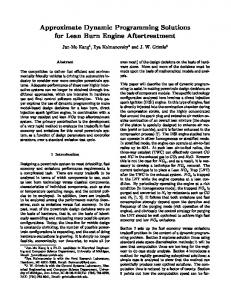
Optimal Primal ALP Composite Primal ALP (singles) Random Worst

800

Relative Complexity

Policy Value

1000

600 400 200 0

4

5

6

7

8

9

Number of features (computers)

(a) Fig. 1.

10

600 500

2

10

1

10

10

Optimal Primal ALP Composite Primal ALP (singles) Random Worst

400 300 200

0

10

−1

3

Exact LP / Composite ALP Primal ALP (doubles) / Composite ALP Primal ALP (singles) / Composite ALP

3

10

Policy Value

1200

100 3

4 5 6 7 8 9 Number of features (computers)

10

0

4 6 8 Number of features (computers)

10

(b) (c) Quality, unidirectional ring (a); Relative efficiency (b); Quality, bidirectional ring (c)

[1, T ], which is assumed to be additively-decomposable (7), just like the reward function r.

5. E XPERIMENTAL E VALUATION The main driving force behind the composite ALP was to construct an efficient ALP, suitable for constrained MDPs, but the approach can certainly also be applied to unconstrained problems. Therefore, since there is a wider variety of algorithms for unconstrained MDPs, we focus on unconstrained domains in our analysis. This ignores one of the advantages of the composite ALP, but gives a more direct and clear comparison to other methods. We evaluated the composite ALP on several domains, including the “SysAdmin” problem (Guestrin et al., 2003), the results for which we report here. The domain involves a network of n computers, each of which can fail with a probability that depends on the status of neighboring computers. The state of the system is defined by n binary features, where each feature defines the status of one computer. At each time step, the decision-maker can reboot a computer and receives a reward that is proportional to the number of computers that are up and running. Figure 1a compares the values of policies for a problem with a unidirectional-ring network The values of policies obtained by the following methods are given: 1) Optimal, 2) Primal ALP3 with basis functions over all pairs of features (quadratic), 3) Composite ALP with the same primal basis, and dual basis over neighbor triplets (linear), 4) Primal ALP with basis functions over single features (linear), 5) Random policy, 6) Worst policy. We performed no optimizations of the bases, and only used very simple functions, such as constants, binary indicators, and identity matrices. The plot shows the actual values of policies (not 3 Note that, for unconstrained problems, the primal ALP (9) is equivalent to the DALP (10).

the value functions), which is a more accurate metric, as constraint approximation in the composite ALP can lead to unrealizable value functions.4 Figure 1b shows the efficiency gains of the composite ALP, relative to the exact LP and the two primal ALPs variations. A problem where each pair of variables appears in at least one function has an induced width that equals the total number of state variables. Thus, the composite ALP achieves exponential speedup, compared to a primal ALP or a DALP with a basis set defined on all pairs of features, but without a significant loss in quality (Figure 1a). The complexity of the composite ALP in these experiments roughly matches the complexity of the primal ALP (or the DALP) with basis functions over single features (Figure 1b), but the composite produces noticeably better policies (Figure 1a). Of course, for more-structured problems, basis functions over single features might suffice, for the more symmetric bidirectional-ring network (Figure 1c). A successful deployment of the composite ALP hinges on the ability to construct good basis functions. The problem of basis selection is outside the scope of this paper,5 but our preliminary experimental investigation suggests that, for many domains, simple and intuitive basis functions perform quite well. We performed experiments on domains with weakly-coupled tasks, using a very simple and intuitive approach to basis function construction: in the spirit of (Poupart, Boutilier, Patrascu, & Schuurmans, 2002), we used optimal solutions (v ∗ and x∗ ) to subproblems with 4

Given the same primal basis, the composite ALP will, in general, produce lower-quality solutions than the primal ALP, because it also approximates the feasible region. The data point in Figure 1a, corresponding to 10 computers, is unusual. The value function of the composite ALP maps to a better policy than a more accurate value function of the primal ALP. 5 For a discussion of the complexity and heuristics for basis selection for the primal ALP, see (Patrascu et al., 2002).

small combinations of subtasks as basis functions (H and Q) for the original problems. Our preliminary results indicate that this approach is promising and yields highquality approximations.

6. D ISCUSSION , C ONCLUSIONS , AND F UTURE W ORK Our main motivation in this work has been to develop a tractable approximation to constrained MDPs, for which exact solutions are predominantly based on the dual LP (2). The sole previous ALP formulation based on the dual LP is Guestrin’s DALP (Guestrin, 2003). As discussed in Section 3, DALP unfortunately scales exponentially with the induced width of the cluster graph, which can be quite large, especially for constrained problems. We have presented the composite ALP approach as a more tractable yet still effective alternative that approximates both the optimization variables and the feasible regions of the LPs, symmetrically handling both the primal and dual variables. The composite ALP can also be effective in solving unconstrained MDPs, as we have empirically shown in Section 5. Overall, our experiments confirm the intuition behind composite ALPs: if the objective function is approximated, then using the exact feasible region can be wasteful. In the future, we would also like to establish more definitive quality bounds for the approach. An alternative feasible-region approximation technique, which statistically samples the constraint set, was proposed by de Farias and Van Roy (2003). However, applying this idea to the dual formulation is problematic, since computing the coefficients for a given constraint in the ADLP (11) is computationally difficult, as demonstrated in Section 3. For unconstrained problems, a careful comparison of the constraint sampling scheme to the composite ALP is an interesting direction for future work, but a direct comparison is difficult, because, even given the same primal basis H, the performance of the two algorithms can vary greatly depending on the choice of constraintapproximation parameters (sampling distribution and the dual basis Q). Another possible way of approximating dual LPs for problems with large induced cost-network widths is to use the DALP (11) with marginal occupation measures that are not globally consistent, as suggested by Guestrin (2003). This idea (and its comparison to our composite ALP) deserves future study.

7. ACKNOWLEDGMENTS This material is based upon work supported by Honeywell International, and by the DARPA/IPTO COORDINATORs program and the Air Force Research Laboratory

under Contract No. FA8750–05–C–0030. The views and conclusions contained in this document are those of the authors, and should not be interpreted as representing the official policies, either expressed or implied, of the Defense Advanced Research Projects Agency or the U.S. Government. Thanks to the anonymous reviewers for helpful comments and suggestions. R EFERENCES Altman, E. (1999). Constrained Markov Decision Processes. Chapman and HALL/CRC. Bellman, R. (1961). Adaptive Control Processes: A Guided Tour. Princeton University Press. Bertele, U., & Brioschi, F. (1972). Nonserial Dynamic Programming. Academic Press. Boutilier, C., Dearden, R., & Goldszmidt, M. (1995). Exploiting structure in policy construction. In Proceedings of the Fourteenth International Joint Conference on Artificial Intelligence, pp. 1104–1111. Morgan Kaufmann. de Farias, D. P., & Van Roy, B. (2003). The linear programming approach to approximate dynamic programming. Operations Research, 51(6). de Farias, D., & Van Roy, B. (2004). On constraint sampling in the linear programming approach to approximate dynamic programming.. Mathematics of Operations Research, 29(3), 462–478. Dean, T., & Kanazawa, K. (1989). A model for reasoning about persistence and causation. Computational Intelligence, 5(3), 142–150. Dolgov, D. A., & Durfee, E. H. (2004a). Graphical models in local, asymmetric multi-agent Markov decision processes. In Proc. of the Third Int. Joint Conf. on Autonomous Agents and Multiagent Systems (AAMAS-04). Dolgov, D. A., & Durfee, E. H. (2004b). Optimal resource allocation and policy formulation in loosely-coupled Markov decision processes. In Proc. of the 14th Int. Conf. on Automated Planning and Scheduling. Guestrin, C., Koller, D., Parr, R., & Venkataraman, S. (2003). Efficient solution algorithms for factored MDPs. Journal of Artificial Intelligence Research, 19, 399–468. Guestrin, C. (2003). Planning Under Uncertainty in Complex Structured Environments. Ph.D. thesis, Computer Science Department, Stanford University. Kallenberg, L. (1983). Linear Programming and Finite Markovian Control Problems. Math. Centrum. Koller, D., & Parr, R. (1999). Computing factored value functions for policies in structured MDPs. In Proceedings of the Sixteenth International Conference on Artificial Intelligence IJCAI-99, pp. 1332–1339. Patrascu, R., Poupart, P., Schuurmans, D., Boutilier, C., & Guestrin, C. (2002). Greedy linear value-approximation for factored markov decision processes. In Eighteenth national conference on Artificial intelligence, pp. 285–291. American Association for Artificial Intelligence. Poupart, P., Boutilier, C., Patrascu, R., & Schuurmans, D. (2002). Piecewise linear value function approximation for factored mdps. In Eighteenth national conference on Artificial intelligence, pp. 292–299. American Association for Artificial Intelligence. Puterman, M. L. (1994). Markov Decision Processes. John Wiley & Sons, New York. Schweitzer, P., & Seidmann, A. (1985). Generalized polynomial approximations in Markovian decision processes. J. of Math. Analysis and Applications, 110, 568 582.