Synchronization and sampling in wireless adaptive signal processing

Ŕ periodica polytechnica Electrical Engineering 54/1-2 (2010) 59–70 doi: 10.3311/pp.ee.2010-1-2.06 web: http:// www.pp.bme.hu/ ee c Periodica Polytechnica 2010

Synchronization and sampling in wireless adaptive signal processing systems György Orosz / László Sujbert / Gábor Péceli

RESEARCH ARTICLE Received 2010-05-25

Abstract This paper deals with the synchronization in wireless adaptive signal processing systems. Wireless communication offers high flexibility, however, the distributed structure of wireless systems requires the synchronization of the subsystems. The synchronization becomes particularly important if the signal bandwidth is in the kHz range, and it is inevitable in distributed control systems. The demand on the synchronization is presented through the introduction of a wireless active noise control system. In this system wireless sensors (microphones) receive the signal, and the main signal processing algorithm is implemented on a central unit which produces the signal for the actuators (loudspeakers). In spite of the special application, the system has a general structure, so the results are valid for other adaptive systems. First a PLL like algorithm is described for the synchronization of the sampling in a wireless real-time signal processing system, then a higher-level synchronization is introduced for a distributed Fourier-analyzer based noise control system. The effectiveness of the algorithms is demonstrated by measurement results. Keywords Synchronization · Digital signal processing · Distributed signal processing · Wireless sensors · Real-time adaptive signal processing Acknowledgement This work is connected to the scientific program of the “Development of quality-oriented and cooperative R+D+I strategy and functional model at BME” project. This project is supported by the New Hungary Development Plan (Project ID: TÁMOP-4.2.1/B-09/1/KMR-2010-0002).

György Orosz László Sujbert Gábor Péceli Department of Measurement and Information Systems, 1117 Budapest, Magyar Tudósok krt. 2, building I, Hungary

Synchronization and sampling in wireless adaptive signal processing systems

1 Introduction

Due to the rapid development in the technology, wireless sensor networks (WSN) become more and more wide-spread in every field of our life, and further growth in the number of potential applications of wireless devices can be expected [1, 30]. Wellknown fields of the utilization of WSNs are, e.g., environmental monitoring, disaster forecast, health care, agriculture, security, military applications, traffic control, production automation [1]. The advantages of wireless technology are, e.g., flexibility, scalability, costeffectiveness, easy deployment, installation and maintenance [2]. In certain cases, wireless communication is more reliable than wired communication links since it is not subjected to some typical problems that emerge in wired systems, e.g., cable breaking. Because of these attractive features of WSNs and the permanent decreasing of their price, the deployment of sensor networks is also promising in such applications where their utilization has many open questions yet. One of these fields is the application of WSNs in real-time, closedloop signal processing and control systems [4, 13, 15, 18, 25, 31]. The application of WSNs for signal processing poses plenty of problems, which are not present in traditional wired systems. Perhaps the most unpleasant one is the uncertain amount of delay in the data transmission [25] which is caused primarily by the network protocol and routing. The system should tolerate missing or faulty samples or possibly missing packets containing many samples. Nevertheless, the nodes of the WSN are responsible not only for collecting samples but processing them, i.e. each node has its own processing unit with its own clock generator. Different clock rates result in different sampling frequencies, which results in inconsistent sampling in the network. The latter problem can be solved by the synchronization of the network nodes [26]. The typical configuration of a wireless feedback signal processing and control system is shown in Fig. 1. Nowadays, typical applications of WSNs in the field of process control is generally the control of slow processes (e.g., temperature) or the so-called open-loop control where sensors supply only auxiliary information about the process to be controlled (e.g., the temperature of a rotating machine) that are used for the fine tuning of

2010 54 1-2

59

The paper is structured as follows. In Section 2, the hardware and software configuration of the wireless active noise control sensor1 system is presented. Section 3 briefly discusses the ANC probMIMO Wireless Signal− sensor2 plant Network processing lem, and summarizes the challenges of its implementation in a sensorN wireless environment. Following the overview of the possible synchronization alternatives, in Section 4, a PLL like synchrofeedback signals nization mechanism is introduced that is used for the synchronization within the wireless network. In Section 5, two pilot Fig. 1. Typical configuration of wireless closed-loop systems Figure 1: Typical configuration of wireless closed-loop systems applications are presented, and special emphasis is put on the synchronization algorithm between the central unit and the senThe application of WSNs for signal processing poses plenty of problems, which are the control algorithm [18]. not present in traditional wired systems. Perhaps the most unpleasant one is the unThis paper focuses on the problem of the synchronization of sors. control signals

certain amount of delay in the data transmission [25] which is caused primarily by the network andnodes routing. The system should tolerate missing or faulty samples or theprotocol network in closed-loop, real-time applications particupossibly missing packets containing many samples. Nevertheless, the nodes of the WSN 2 System description larly in adaptive processing systems. Multi-hop are responsible not only forsignal collecting samples but processing them, i.e. networks each node has its own processing unit with its of ownfaulty clock generator. Different clock rates result different 2.1 Hardware configuration and the correction packets are not considered. Theinissampling frequencies, which results in inconsistent sampling in the network. The latter The block diagram of the wireless active noise control system suecanofbesynchronization will be introduced by nodes a wireless problem solved by the synchronization of the network [27]. active can be seen in Fig. 2. The system consists of two main kinds of The typical configuration a wireless[10, feedback processing andwith control noise control (ANC)of system 14]. signal We do not deal thesystem is shown in Fig. 1. Nowadays, typical applications of WSNs in the field of process control units. ANCthe problem detail, but we usetemperature) it to demonstrate the probis generally control in of slow processes (e.g., or the so-called open-loop controllems wherethat sensors supplyin only auxiliary information aboutapplication. the process to be controlled The computationally critical signal processing algorithms emerge a real-time, closed-loop ANC (e.g., the temperature of a rotating machine) that are used for the fine tuning of the control are implemented on a DSP board which is an ADSP EZ-KIT systems algorithm [18]. are used for the suppression of acoustic disturbances by evaluation board [2]. The processor is an ADSP 21364 This paperof focuses on the problemof of the the destructive synchronization of the network nodesLITE in means the phenomenon interference. The closed-loop, real-time applications particularly in adaptive signal processing systems. (SHARC) DSP which has a 32 bit floating point dual arithmetic noise to be and suppressed is sensed microphones, and theThe so-issue of Multi-hop networks the correction of faultyby packets are not considered. unit and operates with the clock frequency of 330 MHz. The synchronization will be introduced by a wireless active noise control systemis[10,14]. called anti-noise is radiated by loudspeakers. The(ANC) anti-noise We do not deal with the ANC problem in detail, but we use it to demonstrate the probDSP is connected to an AD1835 codec that has two analog ingenerated soa that it minimizes total power of the acoustic lems that emerge in real-time, closed-loop the application. ANC systems are used for the put and eight analog output channels through which the signals suppression disturbances bypositions. means of theIn phenomenon of theANC destructive noiseofatacoustic the microphones’ our wireless sys- interference. The noise to be suppressed is sensed by microphones, and the so-called anti-noise can be fed to the loudspeakers. The analog inputs can be used tem the noise is sensed by wireless sensors.soSince acoustic is radiated by loudspeakers. The anti-noise is generated that itthe minimizes the total as auxiliary input signals, for example, lots of ANC algorithms power systems of the acoustic at the microphones’ positions. In our wireless (MIMO) ANC system the are noise generally multiple-input multiple-output noise is sensed by wireless sensors. Since the acoustic systems are generally multiple-input use a so-called reference signal that carries information about structures, the synchronization is inevitable.is inevitable. multiple-output (MIMO) structures, the synchronization the noise. A question arises, why ANC is chosen application. has been found A question arises, why ANCasis test chosen as test It application. It that ANC has several benefits which make it particularly suitable for test purposes. Although The acoustic signal is sensed by the elements of the wireless beenrelated foundto that ANCproblems, has several benefits which make for it other ANC has is closely acoustical the results can be generalized sensor network which is composed of Berkeley micaz motes physical systems, as suitable well. Thefor advantageous features of ANC asANC test application particularly test purposes. Although is closelycan be [8]. These motes are intelligent sensors that consist of an ATsummarized as follows. to acoustical problems, the results can be generalized for and Anrelated ANC system is easy to install. Sensors and actuators, i.e. microphones mega128 [3] eight bit microcontroller with a clock frequency loudspeakers are commercial products they are easily available. Thefeatures plant is anof acoustic other physical systems, assowell. The advantageous system which is present everywhere and does not require designing and fabricatingof of 7.3728 MHz, a CC2420 2.4 GHz ZigBee compatible radio ANC as test application cansystems. be summarized electrical, mechanical, chemical, etc. The systemasisfollows. flexible: the structure of

An ANC system is easy to install. Sensors and actuators, i.e. 2 microphones and loudspeakers are commercial products so they are easily available. The plant is an acoustic system which is present everywhere and does not require designing and fabricating of electrical, mechanical, chemical, etc. systems. The system is flexible: the structure of the system can be changed by simple geometrical rearrangement, so an algorithm can be tested in different system configurations. An ANC system is a MIMO system. It consists of several microphones and loudspeakers, so a real sensor network can be built using wireless microphones. The loudspeakers are connected to the controller by wires since they need more power than the microphones. An ANC system is scalable. The number of microphones and loudspeakers in the ANC applications vary in a wide range, from single input - single output (SISO) systems to bigger ones, in which 1-2 dozens of microphones sense the acoustic field. Complicated algorithms can be tested with simple systems, but other, well-understood procedures can be checked out in a challenging MIMO environment.

60

transceiver and an MTS310 sensor board [8]. The data transfer rate of the transceiver IC is 250 kilobit per second (kbps) including a preamble section, a header and a footer that are handled by hardware. The sensor board also includes a microphone with a variable gain amplifier whose output signal is converted by the 10 bit analog to digital converter (ADC) of the microcontroller.

mote1

Noise source

mote2

moteN

DSP board

codec reference signal

DSP

mote0

PC

Fig. 2. Block diagram of the wireless ANC system

Figure 2: Block diagram of the wireless ANC system

Most of motes (mote1 . . . mote N in Fig. 2) are responsible

which also serves as a power supply and RS232 line driver for the gateway mote. The P is used for the processing of data sent by the gateway or the DSP over serial port. Per. Pol. Elec. Eng. An independent loudspeaker driven by György Oroszgenerator / László Sujbert / Gábor Péceli a signal is used to generate extern sound. It can be used as an artificial noise source for testing the ANC system or as gene excitation signal for test purpose.

for noise sensing. They transmit the noise data towards the DSP. Data from the wireless network are forwarded to the DSP by the gateway mote (mote0 in Fig. 2). The DSP and the gateway mote are connected to each other via the asynchronous serial port. The data rate of the communication between the two units is 115.2 kbps. The programming of the motes is carried out with an interface board of type MIB510 [8] which also serves as a power supply and RS232 line driver for the gateway mote. The PC is used for the processing of data sent by the gateway or the DSP over serial port. An independent loudspeaker driven by a signal generator is used to generate external sound. It can be used as an artificial noise source for testing the ANC system or as general excitation signal for test purpose.

• Closed-loop systems require deterministic and as low delay as possible. • The system requires continuous data flow, and the blocking of the data flow because of the retransmission of lost packets is not advantageous since it causes the uncertainty of the delay. • The retransmission of the packets requires extra time gaps. These extra time gaps decrease the achievable bandwidth, which is not advantageous since the sensing of the acoustic signal requires high bandwidth. • Simulations and analytical results show that adaptive closedloop systems tolerate well the random data loss that is characteristic of wireless communication, for example randomindependent (i.e. Bernoulli) or random-bursty (i.e. GilbertElliot) [21] data loss.

2.2 Software and network configuration

The operation of the DSP and the motes is time triggered. This means that the signal processing on the DSP is performed with the periodicity Ts DS P , and the sampling, basic signal processing and communication tasks on the motes are performed with the periodicity Tsm . This scheduling scheme is realized using the own timers of the units. The time triggered scheduling ensures the deterministic operation of the system which is important because of the stability of the algorithms that are implemented in the system [15]. The only asynchronous task is the processing of the messages that are sent between the nodes of the system. Since these messages have crucial role in the synchronization, special emphasize must be put on the detection of the arrival time of radio messages during the software development. The system uses single-hop star topology, i.e. the sensor nodes and the base station communicate directly with each other. The network uses Time Division Multiple Access (TDMA) scheme since the real-time operation of the system requires deterministic network protocol and medium access. It has been demonstrated in [16] that TDMA medium access provides better performance in the wireless closed loop systems than random access MAC protocols even with collision detection and avoidance. One can also find standard protocols for sensor networks that support TDMA MAC, for example in ZigBee the beaconenabled mode with guaranteed time slots (GTS) can be used for TDMA communication [5, 6]. Furthermore, TDMA ensures the high utilization ratio of the wireless channel. The network uses UDP like data transmission, i.e. no acknowledge signal is used for the detection of the packet loss. It results in higher data loss ratio than TCP like data transmission (where packet loss detection and correction is used), however, it suits better to the hard real-time behavior of the system. It shows similarities with video and sound streaming in multimedia applications where UDP is also favorable. The following considerations led to the choice that the handling of packet loss is neglected in the network protocol.

Synchronization and sampling in wireless adaptive signal processing systems

3 Active noise control 3.1 Introduction to active noise control

The purpose of ANC systems is to suppress low frequency acoustic noise by means of the destructive interference [10, 14]. Effective noise suppression can be achieved for noises of bandwidth about 1-2 kHz. ANC systems can also be regarded as control systems where the plant to be controlled is an acoustic system, the inputs of which are the loudspeakers that radiate the so-called anti-noise, and the outputs are the signals of microphones that sense the acoustic signals. The plant incorporates not only the acoustic system but also the wireless sensors and network delay. They are described altogether by a matrix A(z) which consists of the transfer functions between each output and each input of the noise control algorithm. A(z) is often called secondary path in the ANC systems. Since the acoustic environment is time varying, adaptive signal processing algorithms have to be used. In the ANC algorithms, a kind of inverse model of the matrix A(z) is applied which is denoted by W(z). In order to ensure the stability of the system, W(z) is often chosen as follows [9, 29]: W(z) = A(z)# ,

(1)

#

where denotes the pseudo- (or Moore-Penrose) inverse. The secondary path A(z) should be identified in advance. The stability criterion of the system is [14, 29]: −

π π < arc(λl ) < , 2 2

λl = λl (A(z)W(z));

l = 1 . . . L,

(2) (3)

where L is the number of inputs. (2) and (3) mean that all eigenvalues λl of the term A(z)W(z) must have positive real part for each frequencies where the noise is present. For the single channel case (only one microphone and one loudspeaker are used) it means that the phase shift of A(z) must be known at least with the accuracy of 90◦ . In practice, it is a crucial problem to ensure the permanency of A(z). 2010 54 1-2

61

3.2 Difficulties in the wireless ANC

Tsm The problems that emerge in ANC applications are generally ti ti+1 ti+2 mote i present in closed-loop signal processing systems. ANC systems t Ttr Ttr are generally multiple-input multiple-output (MIMO) systems, which means that even 1-2 dozens of sensors can be used for tn+3 tn DSP noise sensing. The high number of sensors is required in ort der to achieve effective noise suppression in large space. FurTd1 TsDSP Td2 thermore, ANC systems are real-time signal processing systems which require relatively fast data flow, so they maximally exploit Fig. 3. The changing delay without synchronization the resources of the wireless sensor network from the viewpoint Figure 3: The changing delay without synchronization of the communication and computation. The realization of the noise sensing with wireless sensors re- delay changes, A(z) also changes continuously during the operation so it the differs from its identified W(z) is no of the (i.e. scheduler) of thevalue. units.Hence, According to Fig. 3 quires the accurate synchronization of the tuning sensors, since theyclock can occur that W(z) not satisfy Tsm = TsDSPmore andoptimal. Td1 =Moreover, Td2 = itconst. should be does ensured. It is call must provide consistent information for thethat central controller. the stability condition. example, even intervalinfluenc the events (e.g.,For sampling) mustone besample physically Taking into account that the bandwidth ofsynchronization, the noise may be since (Ts DSfor in the delay causes 90◦ phase shift at a signal Another approach the synchronization is the interpolation, where the e P ) change some kHz, the accuracy of the synchronization must be at least frequency of f = f stime which causes the instability ofby a compu unaligned sampling and processing are compensated DS P /4,instants in some ten µsec range. SISO system. of the interpolation, the exact value of the signal can be estimated at a ANC systems are extremely sensitive tomeans the change of the The synchronization that isdelay. requiredThe for the proper operation so eliminating the changing interpolation is a very g transfer function matrix A(z). Each elementtime of theinstant, matrix A(z) of the system can be solved with different methods [20]. The several applications, so it has very wide literature [7, 19, 23, 28] is a high-order transfer function, the phase ofemerging which can in change units can be synchronized fixingLagrange, the relativeHermite positions polynomia of methods are, e.g., polynomial interpolationby(e.g., rapidly in frequency, thus, in spite of the simplicity of (3), small the time instants of the sampling and signal processing, which squares fitting of polynomials, splines), sinc interpolation or interpolation by changes in the transfer function (e.g., frequency shift of a zero) requires can the tuning of the clock the scheduler) of the signal. The often interpolation be interpreted as (i.e. the conversion of the sampling can cause the instability of the algorithm. Such changes units. According to Fig. 3, it means that T = T and between the sensors and the DSP, so standard methods that are used in th sm s DS P occur in acoustic systems. On the other hand, the presence of also be efficiently realization of integer interpolation Td1 =e.g., Td2 = const. should be ensured. It is called using physicalfiltering the wireless communication increases the uncertainty in the sys- used, polynomial interpolation [7, 23]. The main requirement in the closed-loop sy synchronization, since the events (e.g., sampling) must be phystem by the network induced delay. As it will be highlighted in ensure that the interpolation introduces as low delay as possible while it provid ically influenced. the next sections, the improper synchronization also contributes precision. Another approach for the synchronization is the interpolation, to the delay, so it increases the risk of the instability. The interpolation can realized either onsampling the motes or on the time DSP. In th where thebe effect of the unaligned and processing the DSP acquires the data asynchronously, and the motes calculate the instants are compensated by computation. By means of the in- signal 4 Synchronization request time instants. This means the distributed terpolation, the exactthat value of computation the signal can beisestimated at an in the n 4.1 General considerations the transmission of request messages causes extra load for the network. In the s arbitrary time instant, so eliminating the changing delay. The synchronization is a crucial task in the system because the (each motes send asynchronously, thetask DSP estimates the value o The interpolation is a veryand general emerging in several of the autonomous operation of the subsystems mote and the data in the processing points according to the previous samples and the time of th applications, so it has very wide literature [7, 19, 23, 28]. Stanthe DSP). If the sampling on the motes and the processing of the the data. With this method, the interpolation leads to high computational sampled data on the DSP occurred independently of each other, dard methods are, e.g., polynomial interpolation (e.g., Lagrange, DSP since from every mote or should be handled Hermite polynomials, least-squares fitting individually. of polynomials,The me the delay between the sampling and the processing of the the signaldata interpolation can be chosen in both cases according to trade-offs com sigwould vary at least within one sampling period long interval. splines), sinc interpolation or interpolation by filtering thebetween complexity and Algorithms ensure lower nal. The interpolation canthat be interpreted as the distortion conversion ofof the s The phenomenon of the changing delay is illustrated in Fig. 3. precision. generally require more processor capacity. At the present state thesotechnolo DSP, Let us consider the case when the motes are sampling the noise the sampling frequencies between the sensors and theof to implement complicated interpolation algorithms on the sensor no standard methods that are used in this field can also be effisignal, they send these data to the DSP, andrealistic the DSP processes of their computational, energy and memory constraints. the most recent samples received from motes. A sample can ar- ciently used, e.g., realization of integer interpolation using filrive at any time instant between the actual and the previous data tering followed by polynomial interpolation [7, 23]. The main the closed-loop systems is to ensure that the inprocessing points of the DSP. The delay between sampling requirement in of 4.2 theSynchronization the Sampling terpolation introduces as low delay as possible while it provides and the processing of data at the time instant tn is (Ttr + Td1 ), 4.2.1 Algorithm Description and the delay at the time instant tn+3 is (Ttr + Td2 ). The two sufficient precision. The interpolation can be realized either onstages: the motessynchronization or on the delays are different, which is the result of theIn different sampling our system the synchronization is divided into two DSP. In the first case, the DSP acquires the datanetwork asynchronously, and signal processing frequencies. In the figure, Ttr denotes the and sensor network, synchronization between the sensor and the DSP and the motes calculate the signal value at the request time intransmission time of one sample, the horizontal axes time stages arearereasonable because of the different configuration, functionality an stants. This means that the computation is distributed in the axes, and the short vertical lines denote theofsignal processing the motes and the DSP. network but the transmission of request messages causes extra and sampling instants. A delay 1T contributes to the transfer function A(z) of the load for the network. In the second case, the motes send the data 7 the value of the signal in feedback path by a phase shift e− ω1T . Since A(z) includes asynchronously, and the DSP estimates the delay between the arrival and the processing of data, if the the processing points according to the previous samples and the 62

Per. Pol. Elec. Eng.

György Orosz / László Sujbert / Gábor Péceli

time of the arrival of the data. With this method, the interpolation leads to high computational load on the DSP since the data from every mote should be handled individually. The method of the interpolation can be chosen in both cases according to tradeoffs between computational complexity and precision. Algorithms that ensure lower distortion of the signal shape generally require more processor capacity. At the present state of the technology, it is not realistic to implement complicated interpolation algorithms on the sensor nodes because of their computational, energy and memory constraints. 4.2 Synchronization of the sampling 4.2.1 Algorithm description

edge of which the sampling is carried out. The synchronization of the sampling frequency on the motes is achieved by holding the phase difference between the sawtooth signals constant with a PLL like structure that can be seen in Fig. 4. Since the falling edges of the sawtooth signals represent the sampling points, this algorithm ensures the sinchronization of the sampling.

reference timer

fquartz

reception time instants of the messages: Nl

ref

fquartz

i

Ndiv tuneable In our system the synchronization is divided into two stages: controller S/H timer synchronization within the sensor network, and synchronization Nl − between the sensor network and the DSP. These two stages are Na reasonable because of the different configuration, functionality and resources of the motes and the DSP. In this subsection, the synchronization of the sampling within Fig. 4. Block diagram of the synchronization algorithm. Sawtooth signal the sensor network is presented. The synchronization between Figure 4: Block with diagram of the synchronization algorithm. Sawtooth signal w solid line: reference counter’s value. Sawtooth signal with dotted line: the the sensor network and the DSP depends also on the reference ANC algo-counter’s line: value. Sawtooth signal with dotted line: the value of th value of the counter of the timer to be synchronized. the timer to be synchronized. rithm, so it will be presented together with theofconcrete system architectures. The synchronization is performed in the following way. The The sampling on the motes is physically synchronized. The algorithm requires a reference mote. The reference mote perIn this subsection, the synchronization of the sampling within the sensor physical synchronization is chosen for the motes because it can forms the same tasks as the other sensor motes, but it sends its is presented. The synchronization between the sensor network and the DSP be solved with a simple synchronization algorithm, which is an messages over the radio channel at deterministic time instants also on the ANC algorithm, so it will be presented together with the concret important aspect because of the limited resources of the sensor with constant periodicity that is determined by its timer. Hence, architectures. motes. Physical synchronization of the motes has the sampling supple- these datamotes messages can be usedsynchronized. as synchronization The on the is physically Themessages physical synchr mentary advantage that it makes the timing ofisthe network acand as time reference. At the reception time instants of these chosen for the motes because it can be solved with a simple synchronization a tivity easier, since the motes have the same time reference. messages, the other motes value resources of their ownofcounter. which is an The important aspect because ofread the the limited the sensor mot synchronization of the motes with interpolation is not preferred In Fig. Nl denotes Since the value of advantage the sawtooth that it m ical synchronization of 4,the motes this hasvalue. the supplementary because it increases the complexity and has notiming additional advansignal activity is proportional to its phase, sampling hold (S/H) of the network easier, since thethis motes haveand the same time refere tage. operation is analogous to the phase detector function. Hence, synchronization of the motes with interpolation is not preferred because it incr In order to ensure the synchronization of thecomplexity sampling onand the has withno theadditional tuning of the sampling frequency (changing Ndiv ), the advantage. motes, a PLL like method was developed. The wide-spread In ordersynto ensure synchronization the sampling onthe thereference motes, a PLL lik phasethe difference between theofsawtooth signals on chronization algorithms that are developed forwas sensor networks developed. The synchronization that are developed and wide-spread on the other motes (i.e., Nl ) can bealgorithms kept constant. [11, 12, 17, 26, 27] can not be directly used since they are networks [11,too12, 17,Let 26,N27] can not be directly used since they are too general denote the desired value of N . The synchronization a l general methods, and focus on general time synchronization. and focus onIngeneral time synchronization. In our case, however, the main ta algorithm is as follows: synchronization our case, however, the main task is the synchronization of the of the sampling with high precision. Since we give a special m • ifofNlthe < Nsampling, be increased (i.e., requirement Ndiv should than th a − Ntol , f sm synchronization it should has smaller resource sampling with high precision. Since we give the a special method be decreased) for the synchronization of the sampling, it hasalgorithms. smaller resource The synchronization method a tuneable timer, since synchronization requirement than the general algorithms. • if Nl > Na + Nrequires tol , f sm should be decreased (i.e., Ndiv should by slowing down or speeding up the sampling. The tuneable timer is available o The synchronization method requires a tuneable timer, since be increased) crocontroller of each mote [3]. The timer is realized with a counter which oper synchronization is achieved by slowing down or speeding up the • if of Na the + Ntol ≥ N(f ≥ Na − f sm).should heldcounter on its l quartz tol , clk the clock frequency mote =N1/T Afterbethe has re sampling. The tuneable timer is available on the microcontroller nom nominal value (i.e., N = N ) div programmed maximal value (N ), it is cleared, and an interrupt is generated w div div of each mote [3]. The timer is realized with a counter which 1the microphone’s signal is performed. The value Ndiv determines the ). where Ntol is a tolerance parameter. Ntol is used because of the operates with the clock frequency of the motesampling ( f quartz =ofTclk −1 frequency: f Tsm = fquartz /Ndiv = of 1/(T Ndiv ) (where T is the sampling sm =measurement After the counter has reached its programmed maximal value uncertainty the clk reception time of thesmmessages The time the counter’s value is a sawtooth signal, at the falling edge (Ndiv ), it is cleared, and an interrupt is generated where thefunction sam- (Nof l ), due to the jitter in the communication and software delays. the sampling is carried The synchronization of the sampling frequency on t pling of the microphone’s signal is performed. The value Ndiv Ntol = out. 0 would result in the unnecessary tuning of the timer. f is achieved by holding the phase difference between the sawtooth signals cons −1 = quartz = determines the sampling frequency: f sm = Tsm This is a very simple control algorithm, so it does not require Ndiv 1 (Tclk Ndiv )

a PLL like structure that can be seen in Fig. 4. Since the falling edges of the

(where Tsm is the sampling interval). The time func- considerable computational resources. It is important, since the signals represent the sampling points, this algorithm ensures the sinchronizati tion of the counter’s value is a sawtooth signal, at the falling algorithm is implemented on an eight bit microcontroller.

sampling. The synchronization is performed in the following way. The algorithm r Synchronization and sampling in wireless adaptive signal processing systems 54 1-2 63 reference mote. The reference2010 mote performs the same tasks as the other sensor m 8

A measurement result of the synchronization can be seen in Fig. 5 where the output of the phase detector is observed. As shown by the dashed line in Fig. 5, without synchronization, Nl changes continuously because of the frequency error of the clock generators of the motes. Since the maximal value of the nom , the maximal output signal of the phase deteccounter is Ndiv nom that is in our case 4096. When the motes are tor is also Ndiv synchronized, Nl remains in a ±10 µsec interval around Na that was 3000 (solid line). In the experiment Ntol was set to 32. Since the synchronization messages carry information only in their time of arrival, any data messages can be used for this purpose. The only constraint is that they should be sent by the reference mote at predefined time instants. It means that the synchronization of the sampling in this system means no extra network traffic since it is realized with data messages that should be sent anyway. The synchronization does not need to be performed in each sampling period because the clocks of the motes are accurate enough. In the wireless ANC system every mote is physically synchronized, since in this case the observations of the sensors are consistent. The synchronization of the gateway is required in order to ensure the real-time data forwarding between the network and the DSP (see later sections). 4000

unsynchronized synchronized

3500

N

l

2500 2000 1500 1000 500 50

100 time [sec]

150

Fig. 5. Synchronization measurement results

4.2.2 The effect of packet loss

Since wireless communication systems are prone to packet loss, some considerations are given how to take this effect into account. It is assumed that if a packet is lost by a node, it uses the nominal sampling period, i.e. the synchronization algorithm is inactive. The detection of the packet loss can be solved using a timeout mechanism. The synchronization packets are sent regularly, so the nodes can notice that a synchronization packet is lost by measuring the time elapsed since the last received packet. If this time exceeds a limit, the synchronization should be inactivated. 64

div

1 1 = 244 ppm. used in Section 6, then ρcomp = N nom = 4096 div This is considerably higher than the error of the quartz oscillators. Hence, it is more dangerous to apply a modified sampling frequency than the nominal one if a synchronization packet is lost, since the node to be synchronized is not aware of the error of the synchronization, and it has no information whether a compensation is required or not.

5 Pilot applications

3000

0

The algorithm could be further improved by estimating the drift of the clocks—see e.g., [17], and performing the synchronization in the case of packet loss using this calculated drift. The synchronization should be disabled when a packet is lost because the unnecessary changing of the sampling frequency could cause the overcompensation of the drift which can even increase the error between the clocks. The reason is that the frequency error of the commercial crystal oscillators is in some or at most some ten ppm range, however, if the sampling frequency is changed, it can cause much higher drift compensation. Taking a practical example that is presented in Section 6, the drift between the clocks of two sensor nodes is 555·10−6 sec ρ = 152.8sec−47sec = 5.25 ppm (it is the slope of the sawtooth signal in Fig. 12.(d)). Furthermore, if the synchronization algorithm changes the sampling frequency even to the smallest extent, i.e. the nominal value of the division factor Ndiv is changed nom ±1, it causes a compensating drift approxby one: Ndiv = Ndiv 1 nom = 4096 which is . Assuming that Ndiv imately ρcomp = N nom

Per. Pol. Elec. Eng.

In this section, two kinds of ANC systems are introduced that have already been implemented. Both of them utilize the resonator based ANC algorithm [29], however, the structures of these systems are quite different. These two different structures show the difficulties and advantages of the deployment of wireless sensors. The resonator based ANC algorithm can be used for suppressing periodic noises providing better performance for periodic noises than the general methods [29]. The noise control algorithm requires the exact estimation of the fundamental frequency of the noise that is denoted by f 1 . The frequency f 1 is measured by an adaptive Fourier-analyzer (AFA) algorithm [22] using the reference signal. The reference signal is directly connected to the DSP board, as it can be seen in Fig. 2. The reference signal can be any signal the frequency of which equals to f 1 . The AFA is implemented on the DSP as it requires floating point computations. The two kinds of ANC systems that will be introduced in this section have the same hardware configuration as shown in Fig. 2, the difference lies in the implementation of the ANC algorithm. The sampling frequency on the motes is f sm = 1.8 kHz and f s DS P = 2 kHz on the DSP. The different sampling frequencies are constrained by the hardware and by the bandwidth of the wireless network.

György Orosz / László Sujbert / Gábor Péceli

5.1 ANC with simple data transmission network

In this system an obvious method of the signal observation is used, which means that the motes perform the sampling of the noise, and they transmit the samples to the base station over radio. The base station collects the data from the sensors and forwards one sample from each mote to the DSP at each sampling instant. Since every mote (including also the gateway) is physically synchronized, they provide data with the same average sampling frequency, and the relative positions of the sampling instants on the different motes are fixed. Furthermore, since the gateway is also synchronized, the time difference between the reception and the forwarding of the sensors’ data is constant, so there is no changing delay in the data path. Hence, the whole network can be regarded as a multiple channel compact data acquisition system, and the operation of the sensor network is transparent from the viewpoint of the DSP. The network operation is time division multiplexed (TDM): the motes transmit their data periodically, in predefined order, in their own timeslots. This kind of network protocol is proven to be a suitable solution [15] as the probability of the message collision, data loss and fluctuation in the data transmission time is less than in the case of random access protocols [15]. The sensors send data in 25 samples size packets, and the gateway performs the serialization of the data. The fitting of the sampling frequency of the motes to that of the DSP is achieved by linear interpolation. Linear interpolation is used since it provided sufficient performance in practice, and higher order interpolation would introduce more delay, which is not advantageous in a closed-loop system. The interpolation algorithm is explained in Fig. 6, where f (t) stands for the signal to be interpolated and the dots symbolize its sampled values. The samples are supplied by the motes, and the interpolation is carried out on the DSP. The DSP estimates the signal value at the signal processing point tn as follows: Td Tsm − Td fˆ(tn ) = f (ti−1 ) + f (ti ) . Tsm Tsm

(4)

In order to ensure the causality, one sample delay should be introduced since f (ti ) is not known in tn . With this method, the effect of the continuously changing delay, Td , is alleviated (see Td1 and Td2 in Fig. 3), since the sampling instant of the mote is virtually replaced to tn . 5.2 ANC with distributed signal processing

The bottleneck of the system introduced in the previous subsection is the bandwidth of the wireless network which limits the number of motes at a given sampling frequency. The sampling frequency is determined by the bandwidth of the acoustic signals. To overcome this problem, the signal processing capability of the intelligent sensor nodes was exploited. In order to increase the effective throughput of the network, a transformed domain data transfer was developed. This kind of signal transmission can be applied in the case of periodic Synchronization and sampling in wireless adaptive signal processing systems

f (t) fˆ (tn ) f (ti ) f (ti − 1 )

f (ti − 2 )

Td

tn T sm

Fig. 6. Synchronization with linear interpolation

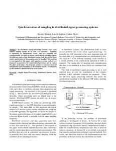
noise. In this system, the sensors realize a distributed Fourieranalyzer algorithm, and they send only the Fourier coefficients of the periodic signals to the DSP. The Fourier coefficients are computed by the motes with an observer based Fourier-analyzer (FA) structure [24]. These coefficients change slower than the signal, so a lower transmission rate can be achieved. Hence, the small communication bandwidth does not mean a hard limit for the number of the sensor motes. This allows the deployment of more motes without decreasing the sampling frequency. The number of motes is limited by the properties of the noise and the performance requirements (e.g., settling time). The assumption that the Fourier coefficients change slowly is true if the parameters of the observed periodic signal yn change slowly or rarely, i.e. at least the short term stationarity of the signal is required. Formally, this means that if yn is composed of si
P nusoidal components, i.e. yn = i ai (n) cos ωi (n)n + φi (n) , then the amplitude, phase and frequency of the ith component do not change considerably between the transmission time instants, or they change rarely. This condition is generally true for acoustic signals that are generated by mechanical equipments (e.g., rotating machines) since the inertia of these systems and the time constants of the mechanical movements do not allow the rapid or frequent change of the parameters of the generated periodic signal (i.e. the noise of the machine). For example, let us assume a 0.1 sec time segment. Due to the physical circumstances, the angular frequency of a machine does not change considerably within this time segment. If a sampling frequency of several kHz is applied, it means that a sensor collects and transmits several hundreds of samples during this time. However, since the frequency does not change considerably in this interval, it is sufficient to send the signal parameters only once. Fig. 7 depicts the structure of a resonator based distributed ANC system. In the original configuration of the algorithm

2010 54 1-2

65

A(z) A(z)

mote 1

mote 1

FA

FA

mote 2

Acoustic plant

Acoustic plant

mote 2 FA

DSP

FA

gateway

moteN

DSP

ANC

gateway

ANC

algorithm

algorithm

moteN

FA

FA

Fig. 7. Distributed Fourier-analyzer based ANC system

Figure 7: Distributed Fourier-analyzer based ANC system Figure 7: Distributed Fourier-analyzer based ANC system

t0

data

DSP synchronization

t′0

radio comm.

serial comm. radio comm.

cn (t) = e

ts

DSP data

serial comm.

[29], the FA and the ANC blocks are implemented on tthe same s hardware, so in this distributed structure a new synchronization synchronization data problem emerges: the consistency of the basis functions of the tr t′0 t0 mote and on Fourier-decomposition has to be ensured on each the DSP, because the phase of the Fourier coefficientsbroadcast can be data synchronization interpreted by the ANC algorithm only by using a common reference in the system. This reference is the basis function set of tu the Fourier-decomposition. The n th basis function is defined as Fig. 8. follows:

tr

base

base broadcast synchronization

data

data mote

1

mote

1

moteN

moteN

tu

Network operation in the distributed ANC system

Figure 8: Network operation in the distributed ANC system t X Figure 8: Network operation in the distributed ANC system  2π[nϕ1 (t)] t ,

ϕ1 (t) =

f 1 (τ )1τ,

τ =0

(5)

defined as follows:

0

base

as the follows: Ttr where ϕ1 defined and f 1 are phase and the frequency of the funt = e2π[nϕ1 (t)] cnX (t) , ϕ1 (t) = Tdif f f1 (τ )∆τ, 2π[nϕ damental harmonic components, respectively. The fundamental 1 (t)] cn (t) = e , ϕ1 (t) = f1 (τ )∆τ, (5) τ =0 frequency of the basis functions equals to the fundamental fresensor where ϕ1 and f1 are theτ =0 phase and the frequency of the fundamental harm quency of the noise. where ϕ1 and f1 are the phase and respectively. the frequencyThe of fundamental the fundamental harmonic components, frequency the basis functions equ tof u The operation of the system is the following. The activity Tsm ponents, respectively. The fundamental frequencyofofthe thenoise. basis functions equals to the fundamental frequency of the wireless network is periodic, each period consists of two fundamental frequency of the noise. The operation of the system is the following. The activity of the wireless n Fig. 9. Synchronization of the basis functions (sensors to base station) phases, as shown in Fig. 8. First, the base station sends a synperiodic, period consists of twoofphases, as shown in Fig.is 8. First, the ba The operation of the system is theeach following. The activity the wireless network chronization message to the motes which is sends used for the synFigure 9: Synchronization of the basis functions (sensors to synchron base sta a synchronization message to the motes which is used for the periodic, each period consists of two phases, as shown in Fig. 8. First, the base station chronization of both the sampling frequency and the basis funcstant t (see Fig. 8), and it includes f (t ) and ϕ (t ) that are the both the sampling 0 1 0 After 1 this 0of message, each sends a synchronization message to the motesfrequency which is and usedthe forbasis the functions. synchronization tions. After this message, each mote gets thethe right in a in predeactual value of the frequency and the phase of the fundamental right a predefined order to transmit the Fourier coefficients to the bas both the sampling frequency and the basis functions. After this eachsynchronization mote gets station and the is depicted in message, Fig. 9. The is carried o fined order to transmit the Fourier coefficients to the base sta-sensors After the synchronization message, the base station begins to forward the data harmonic basis function at the time instant of the transmission the right in a predefined order tosynchronization transmit the Fourier coefficients to station the base station. the message of the base that is sent at the time in tion. After the synchronization message, theofbase station begins from thethe network to the themessage, DSP. of respectively. Let us data denotecollected the transmission inAfter the synchronization message, base station begins to forward the Fig.to 8), it includes f1of(tthe ) and ϕ1functions (t ) that are the actual valuephases. of the frequ to forward the data collected from the network the and DSP. The synchronization basis carried outofin stant of this0 message by 0t0 and theistime instant thetwo utilization The t from the network to the DSP. phase of the fundamental harmonic basis function at the time instant the The synchronization of the basis functionsare carried out in of the information the synchronization between the base station andby the sensors, and bethe of synchr sent in the message tu ,stages so the delay The synchronization of the isbasis functions is carried out in two phases. The two ofbetween the between message, respectively. Let’s denote the transmission instant of this two phases. The two stages are the synchronization the the DSP and the base station. sensors synchronized to tween these two events is (tThus − t0synchronization ).the Since these are operations are uthe are the synchronization between the base station and the sensors, and t0 indirectly, and thebetween time instant of the utilization of the information sent in the m base station and the sensors, and the synchronization through the base station. out at sampling instants, and the on the motes between the DSP and the base station. Thuscarried the sensors are synchronized tosampling the DSP so are the delay between these two events is (tuT − tthe Sinceso these operation The timing diagram of the synchronization of basis functions the DSP and the base station. Thus the sensors synchronized 0=). const), is physically synchronized (i.e. the delaybetween di f f indirectly, through the base station. out at sampling instants, and the sampling on the is physically sync to the DSP indirectly, through the base station. (tu − ) is constant. Hence, thebetween delay (tu motes −the t0 ) can The timing diagram of the synchronization of t0the basis functions basebe regarded Tdifoff the = basis const), delay (t −t ) is constant. Hence, the delay (tu −t0 ) can The timing diagram of the synchronization func-so the u 0 as the part of A(z). 13 as isthe part inofFig. A(z). The phase of the fundamental harmonic basis function can be tions between the base station and the sensors depicted of 13 the fundamental harmonic basis function can be estimated at 9. The synchronization is carried out by meansThe of thephase synchrot in way: nization message of the base station that istime sent at the the timefollowing in66

Per. Pol. Elec. Eng.

t X

ϕ1 (t) = ϕ1 (tGyörgy f1 (t/uLászló )(t −Sujbert tu )./ Gábor Péceli u ) +Orosz

The phase of the nth harmonic basis function is ϕn (t) = nϕ1 (t), becaus value of the phases are zero and the frequencies are in harmonic relation

available time was used for computation of the ANC algorithm on the DS hand, the storage of the transfer function matrix A(z) has large memory The application of the distributed Fourier-analyzer structure that is p estimated at an arbitrary time t in the following way: The application of the distributed Fourier-analyzer structure subsection is not limited ANC systems, butisitnotcan betoused in any ap that to is presented in this subsection limited ANC sysϕ1 (t) = ϕ1 (tu ) + f 1 (tu )(t − tu ). (6) tems, it can be signals used in any where the synthe synchronous analysis ofbutperiodic is applications important (e.g., power sys

The phase of the n th harmonic basis function is ϕn (t) = nϕ1 (t), chronous analysis of periodic signals is important (e.g., power because the initial value of the phases are zero and the frequen- systems). cies are in harmonic relationship, so the synchronization of only 6 Results the first basis function is sufficient. Since the frequency of the In this section, some results are presented which prove that periodic acoustic disturbance to be suppressed ( f 1 ) changes genIn this section, some results are presented prove that the the synchronization is inevitablewhich in a wireless, closed-loop ap- synch erally slowly, it can be regarded constant between two synchroevitable in a wireless, closed-loop application, demonstrate plication, and demonstrate the properand operation of the synchro-the prop nization messages. nization algorithms havebeen been introduced in this paper. synchronization that that have introduced in this paper. The synchronization betweenthe the DSP and the base stationalgorithms 0 begins with the initiation message of the gateway at t0 as it can be seen in Fig. 8 and Fig. 10. At the reception instant of this noise source Signal gen. message (ts ), the DSP calculates the actual value of the phase of the fundamental basis function as follows:

6

Results

ϕ1 (ts ) = ϕ1 (t p ) + f 1 (t p )(ts − t p ),

(7)

mote1

where ϕ1 (t p ) and f 1 (t p ) denote the values of the phase and the frequency in the previous processing point, respectively. The mote0 DSP time diagram can be seen in Fig. 10. ϕ1 (ts ) and f 1 (ts ) are then sent to the gateway which updates its old data with these new ones. This procedure is important because the gateway and the Fig. 11. Measurement arrangement DSP run asynchronously, so the DSP has to estimate the value Figure 11: Measurement arrangement The tests were performed both for the simple data collecting of the phase whenever the gateway initiates the synchronization. The transmission of ϕ1 (t p ) would introduce a changing delay and the distributed ANC systems. The measurements were carThe tests were performed both for the simple data collecting and the d (ts − t p ) into A(z), thus W(z) could not be determined correctly. ried out on a single-input single-output (SISO) system—i.e., one loudspeakerwere and onecarried microphoneout were on used.aThe sampling fre- single systems. The measurements single-input This (ts −t p ) delay is eliminated by the last term of (7). Constant quency wasand set to one f sm =microphone 1800 Hz. The block diagram of the delays of the data transmission (T no trouble system—i.e., loudspeaker were used. The sam tr 1 and Ttr 2 ) causeone physical arrangement can be seen in Fig. 11. A signal generasince they are represented in A(z). was set to fsm = 1800 Hz. The block diagram of the physical arran tor was used as a noise source which was connected to a loudseen in Fig. 11. A signal generator was used as a noise source which speaker. The noise was a sinusoidal signal with the frequency tp ts to a loudspeaker. sinusoidal signal with the frequency DSP The ofnoise 115 Hz.was The a measurements were performed in a laboratory room, the distance the sensor mote and the loudspeaker measurements were performed in abetween laboratory room, the distance betw was about 0.5 m. In order to examine the performance of the the per Ttr2 Ttr1 mote and the loudspeaker was about 0.5 m. In order to examine system, the noise level was measured by an external microphone base system, the noise level was measured by an external microphone that wa that was situated about 1 cm from the noise sensing microphone t′0 tr from the noise sensing 1 cm microphone the were sensor mote, and the signa of the sensor mote, and theof signals recorded by a PC sound card. The transfer function A(z) was measured under normal Fig. 10. Synchronization of the basis functions (base station to DSP) ure 10: Synchronization of the basis functions (base station operating to DSP)conditions, when the synchronization worked propIn the simple data collection system, the maximal applicable erly. 15 number of motes was three, while in the distributed ANC system The basic concept of the measurements is that the noise supistributed signal processing based method. In this the number oftosensors the experimental system consisted of eight motes at case, the same pression is be examined when the synchronization is turned tended up to some dozens. The sizethe ofsignal the network is limited byand theoff. properties sampling frequency. This proves compression capa- on It is expected that the system without synchronizato be suppressed (e.g.,distributed the rate signal of theprocessing change of themethod. noise parameters) by in some seconds as the clock frequencies bility of the latter, based tion becomesand unstable es of theInDSP. However, theofcomputational burdenupmeans restriction this case, the number sensors could be extended to somemarginal differ from each other on the motes. When the synchronization e case of eight motes and four loudspeakers only about five percent of the dozens. The size of the network is limited by the properties of is on, the system remains stable during the whole observation me was the used fortocomputation thethe ANC algorithm On the other noise be suppressed of (e.g., rate of the changeon of the the DSP. period. torage of theparameters) transfer function A(z) has large memory demand. noise and by thematrix resources of the DSP. However, licationthe of computational the distributed Fourier-analyzer structure that in this 6.1 The simple data collecting ANC system burden means marginal restriction since in is presented The synchronization the case of eight motes and four loudspeakers only about five s not limited to ANC systems, but it can be used in any applications where algorithm of this system is described in percent of availablesignals time was for computation of the systems). Section 4.2. By turning off the synchronization in the wireless nous analysis of the periodic is used important (e.g., power ANC algorithm on the DSP. On the other hand, the storage of network, the sampling of the acoustic signal on the sensor and the data forwarding on the base station slide away from each the transfer function matrix A(z) has large memory demand.

ults

Synchronization and sampling in wireless adaptive signal processing systems

2010 54 1-2

ion, some results are presented which prove that the synchronization is ina wireless, closed-loop application, and demonstrate the proper operation of

67

other, which results in the continuous changing of the delay in the feedback path. This phenomenon is explained in Fig. 3. The measurement results are presented in Fig. 12. Fig. 12(a) and (b) belong to the synchronized state, while Fig. 12(c) and (d) belong to the unsynchronized state. In Fig. 12(a) and (c), the time functions of the noise can be seen during the operation of the noise control algorithm. Fig. 12(b) and (d) contain the time functions of the delay, Td , between the events when the base station receives the sensor’s sample and forwards it to the DSP. Note that the time scale in each column is the same, therefore the change in Td and the working of the ANC system can easily be connected. Td is denoted by Tdi in Fig. 3, and it causes an extra phase shift in the transfer function of the feedback path. Theoretically, Td is the only changing delay which can influence the stability of the system. Td can change in the interval of [0 . . . 555] µsec, since the new samples of the sensor are available with the periodicity 1 = 555 µsec, and the gateway forwards the most Tsm = 1800Hz recent sample. In Fig. 12(a) and (b) the time functions can be seen that were recorded when the synchronization worked properly. The delay Td stayed in the neighborhood of the nominal value Td_nom = 400 µsec. Since this is included in the transfer function A(z), the system is stable. The ANC algorithm was started at the time instant of 15 sec, and it reduced the noise level by 26 dB. The algorithm stayed in stable state during the whole observation time. The result is completely different when no synchronization was applied between the sensor and the gateway as Fig. 12(c) and (d) show. In this measurement, the synchronization was active in the first 20 sec, then the synchronization was turned off. The noise control algorithm was started at the time instant of 15 sec. Since the synchronization worked properly, the noise control algorithm achieved the usual suppression. After the synchronization had been turned off, the delay Td began to change, which led to instability. The extra delay that surely causes the instability of the system can be calculated according to (3). The system is the most sensitive at the highest operating frequency where the delay causes the highest phase shift. Since the stability region is at most 1φ = 90◦ , and the highest operating frequency is 805 Hz=115 Hz·7 (the 7th harmonic component), the extra delay which surely causes instability is 1Tcrit = 360◦1φ ·805 Hz = 310 µsec. Note that the crucial delay in practice is a bit less than 1Tcrit . In Fig. 12.(d), the grey area indicates the theoretical instability region where the difference from the nominal delay (Td_nom ) exceeds the critical value (1Tcrit ). The border of this region is: Tcrit = Td_nom − 1Tcrit = 90 µsec. Indeed, one can see in Fig. 12(c) and (d) that the system became unstable after the delay had approached the critical region, and the system recovered from the unstable state after the delay had left the critical region. Since the delay changes continuously, the stable and unstable periods are repeated. 68

Per. Pol. Elec. Eng.

As one can see in Fig. 12, the system remained stable over Tus ≈ 28 sec after the synchronization had been turned off. This measurement also characterizes the synchronization algorithm from the viewpoint of the data loss. The reason is that, as recommended in Subsection 4.2.2, the synchronization should be switched off by a node if a packet is lost. Hence, the time Tus during which the system remains stable with disabled synchronization equals the time interval during which the consecutive loss of the synchronization packets is allowed without losing the stability of the system. In this particular example, several hundred synchronization packets were sent in the network during the time when the synchronization was intentionally disabled and the system became finally unstable, so it has very small probability that in a practical case such an extreme data loss scenario occurs which causes instability. 6.2 The distributed ANC system

The synchronization algorithm of this system is described in Section 5.2. The effect of the unsynchronized operation was tested by turning off the synchronization of the basis functions between the DSP and the base station. Since the sensor gets the synchronization information from the base station, it means that the sensor mote is not synchronized, as well. The measurement results are found in Fig. 13. In this case no internal states are available, only the time functions of the noise are plotted. The measurement result that belongs to the synchronized system can be seen in Fig. 13(a). The noise control algorithm was started at 15 sec, and it was stable during the whole observation time. The noise suppression was 24 dB. Fig. 13(b) shows the measurement result of the unsynchronized ANC system. The noise control algorithm was started at the time instant of 15 sec, and the synchronization was active in the first 20 sec. The system became unstable at about 40 sec which caused increasing noise level. The reason of the instability is that after turning off the synchronization, the phases of the basis functions begin to slide away from each other on the sensor and on the DSP. The difference between the basis functions results in a phase error in the measurement of the Fourier coefficients of the noise that can be interpreted as a phase error in the transfer function. If this phase error exceeds the stability limit (1φ = ±90◦ ), the system becomes unstable. The ANC system produced larger sound during the unstable state than in the normal operating region, so the noise sensing microphone was saturated. The system became stable again in the interval [445 sec . . . 490 sec]. This temporary stability interval appears every time the phase error between the basis functions approaches k · 2π, since the basis functions are periodic with period 2π. Similarly to the simple data collecting system, this phenomenon causes that the stable and unstable intervals are repeated after each other. These measurements prove the long term stability of the operation of the synchronization algorithm, and it can be concluded that the unsynchronized distributed signal processing causes the György Orosz / László Sujbert / Gábor Péceli

sensor and the data forwarding on the the base base station station slide slide away away from from each each other, other, which which results in the continuous changing of of the the delay delay in in the the feedback feedback path. path. This This phenomenon phenomenon is explained in Fig. 3. Synchronization Synchronization off off 11

0.5

0.5 0.5

noise signal signal noise

noise signal signal noise

Synchronization Synchronization on on 1

0 −0.5 −1 −1 0 0

00 −0.5 −0.5

50 50

100 100

150 150

−1 −1 00

200 200

50 50

600 600

600 600

500 500

500 500

400 400

400 400

300 300 200 200 100 100 0 0 0 0

100 100

150 150

200 200

300 300 200 200 100 100

50 50

100 100

time[sec] time[sec] Fig. 12.(c) Fig. c 12.(c)

[µsec] TTdd[µsec]

[µsec] TTdd[µsec]

time[sec] time[sec] Fig. 12.(a) a Fig. 12.(a)

150 150

TTcrit crit

00 00

200 200

50 50

100 100

150 150

200 200

time[sec] time[sec] Fig. Fig. 12.(d) 12.(d) d

time[sec] time[sec] Fig. Fig. 12.(b) 12.(b) b

Figure Figure 12: 12: Measurement Measurement results results in in the the simple simple data data collecting collecting ANC ANC system. system. Fig Fig (a) (a) and and

(c): noise measured by the external on and Fig. 12. Measurement the simple data collecting Fig microphone nization is onwhen and off,synchronization respectively. Fig (b)is delay between the motes (c): results noisein signal signal measured by ANC the system. external microphone when synchronization isand on(d): and

off, respectively. Fig and delay between motes (a) and (c): noise signal by the external microphone when synchrowhenthe synchronization is on synchronization and off, respectively. is off,measured respectively. Fig (b) (b) and (d): (d): delay between the motes when when synchronization is on on and and off, off, respectively. respectively.

Synchronization on

The The1 measurement measurement results results are are presented presented in in Fig. Fig. 12. 12. 1 synchronized state, while Fig. 12.(c) and (d) synchronized state, while Fig. 12.(c) and (d) belong belong 16 16

0

−0.5

−1

0.5

noise signal

noise signal

0.5

Synchronization off

Fig. Fig. 12.(a) 12.(a) and and (b) (b) belong belong to to the the to the unsynchronized state. to the unsynchronized state. In In

0

−0.5

0

100

200

300

400

time[sec] Fig. 13.(a)

500

−1

0

100

200

300

400

500

time[sec] Fig. 13.(b)

a

Figure 13: Measurement results in the distributed ANC system. Fig (a): synchronization is on, Fig (b): synchronization is off.

b

Fig. 13. Measurement results in the distributed ANC system:a: synchronization is on, b: synchronization is off.

improper and unpredictable operation of the system. 6.2 The Distributed ANC

tributed manner by independent sensors. This distributed strucSystem ture of the wireless systems requires accurate synchronization.

The synchronization algorithm of this system isThe described in Section The effect of the frames of two 7 Conclusions synchronization was5.2. introduced within

the unsynchronized operation was tested by turning off the synchronization of the basis In this paper, the issue of the synchronization and sampling variants of a wireless active noise control system. Although functions between the DSP and the base station. Since the sensor gets the synchronization in the wireless, closed-loop systemsitwas in- that ANC acoustic the results informationsignal from processing the base station, means thesystems sensor are mote is notsystems, synchronized, as can be generaltroduced. The sampling, i.e., the signal observation one ofin Fig. ized 13. for any adaptive signal processing A PLL like well. The measurement results areisfound In this case no internal statessystems. are available, only the time system, functions the noise method are plotted. the most basic tasks in a signal processing so itofrequires was introduced which ensures the synchronous samThein measurement that belongs the synchronized can the be seen in special attention. While the centralized result signal processing sys- to pling of the acousticsystem noise with continuous tuning of the Fig. 13.(a). The noise control algorithm was started at 15 sec, and it was stable durtems the simultaneous sampling of the observed signals can be sampling frequency of the motes. The synchronization between ing the whole observation time. The noise suppression was 24 dB. solved easily, in a wireless system the data are collected in a dis- the sensors and the central controller was solved by interpolaFig. 13.(b) shows the measurement result of the unsynchronized ANC system. The noise control algorithm was started at the time instant of 15 sec, and the synchronization was active in the first 20 sec. The system became unstable at about 40 sec which Synchronization and sampling in wireless adaptive signal processing systems 2010 54 1-2 69 caused increasing noise level. The reason of the instability is that after turning off the synchronization, the phases of the basis functions begin to slide away from each other on the sensor and on the DSP. The difference between the basis functions results in a phase

tion. A distributed wireless ANC system was also introduced where the sensors perform the Fourier-decomposition of spatially separated signals in order to achieve data compression. In this case, the synchronization of the basis functions of the Fourier-decomposition has to be solved in order to ensure a global reference in the system. Both synchronization methods were tested with experimental measurements which prove the necessity of the proposed synchronization, and demonstrate the proper operation of the synchronization algorithms. Further research aims at the development of closed-loop multi-hop wireless signal processing systems.

18 Mathiesen M., Thonet G., Aakvaag N., Wireless ad-hoc networks for industrial automation: Current trends and future prospects, Proceedings of the ifac world congress, July 4-8 2005. 19 Meijering Erik, A chronology of interpolation: From ancient astronomy to modern signal and image processing, Proceedings of the IEEE 90 (March 2002), no. 3, 319–342, DOI 10.1109/5.993400. 20 Molnár K., Sujbert L., Péceli G., Synchronization of sampling in distributed signal processing systems, Int. symp. on intelligent signal processing, wisp 2003., Sept. 2003, pp. 21–26, DOI 10.1109/ISP.2003.1275807, (to appear in print). 21 Mushkin M., Bar-David I., Capacity and coding for the Gilbert-Elliot channels, IEEE Transactions on Information Theory 35 (1989), no. 6, 1277–1290. 22 Nagy F., Measurement of signal parameters using nonlinear observers, IEEE Trans. on Instrumentation and Measurement IM-41 (Feb. 1992), no. 1, 152– 155, DOI 10.1109/19.126651. 23 Niemitalo Olli, Polynomial interpolators for high-quality resam-

References 1 Akyildiz I. F., Su W., Sankarasubramaniam Y., Cayirci E., Wireless sen-

pling of oversampled audio, 2001, available at http://www.student.

sor networks: a survey, Comput. Netw. 38 (2002), no. 4, 393–422, DOI

oulu.fi/~oniemita/DSP/INDEX.HTM. 24 Péceli G., A common structure for recursive discrete transforms, IEEE

10.1016/S1389-1286(01)00302-4. R processor family, 2 Analog Devices, Ez-kit lite for the adsp-2136x sharc

Trans. Circuits Syst. CAS-33 (Oct. 1986), no. 10, 1035–1036, DOI 10.1109/TCS.1986.1085844.

Analog Devices Inc., www.analog.com, 2005. R datasheet, Atmel co., www.atmel.com, 2002. 3 Atmel, Atmega128a 4 Baillieul J., Antsaklis P. J., Control and communication challenges in net-

25 Ploplys N. J., Kawka P. A., Alleyne A. G., Closed-loop control over wire-

worked real-time systems, Proceedings of the IEEE 95 (Jan. 2007), no. 1, 9– 28, DOI 10.1109/JPROC.2006.887290. 5 Boughanmi Najet, Song Ye-Qiong, Rondeau Eric, Wireless networked

DOI 10.1109/MCS.2004.1299533. 26 Römer K., Blum P., Meier L., Time synchronization and calibration in wireless sensor networks, Handbook of sensor networks: Algorithms and architectures, 2005, DOI 10.1002/047174414X.ch7, (to appear in print). 27 Römer K., Time synchronization in ad hoc networks, Mobihoc ’01: Proceedings of the 2nd acm international symposium on mobile ad hoc networking

control system using IEEE 802.15.4 with GTS, 2nd junior researcher workshop on real-time computing, JRWRTC 2008, 16-17 Oct. 2008. 6 Choi Dong-Hyuk, Kim Dong-Sung, Wireless fieldbus for networked control systems using LR-WPAN, International Journal of Control, Automation and Systems 6 (Feb. 2008), no. 1, 119–125. 7 Crochiere R. E., Rabiner L. R., Multirate digital signal processing, Englewood Cliffs, NJ: Prentice-Hall, 1983. 8 Crossbow, Crossbow products overview, Crossbow Technology Inc., www. xbow.com, 2005. 9 Elliott S. J., Boucher C. C., Nelson P. A., The behavior of a multiple channel active control system, IEEE Trans. on Signal Processing 40 (May 1992), no. 5, 1041–1052, DOI 10.1109/78.134467. 10 Elliott S. J., Nelson P. A., Active noise control, IEEE Signal Processing Magazine 10 (Oct. 1993), no. 4, 12–35, DOI 10.1109/79.248551. 11 Elson J., Girod L., Estrin D., Fine-grained network time synchronization using reference broadcasts, Osdi ’02: Proceedings of the 5th symposium on operating systems design and implementation, Dec. 2002, pp. 147–163, DOI 10.1145/844128.844143, (to appear in print).

less networks, IEEE Control Systems Magazine 24 (Jun. 2004), no. 3, 58–71,

& computing, Oct. 2001, pp. 173–182, DOI 10.1145/501416.501440, (to appear in print). 28 Schafer R. W., Rabiner L. R., A digital signal processing approach to interpolation, Proceedings of the IEEE 61 (June 1973), no. 6, 692–702, DOI 10.1109/PROC.1973.9150. 29 Sujbert L., Péceli G., Periodic noise cancellation using resonator based controller, Proceedings of the active ’97, the international eaa symposium on active control of sound and vibration, Aug. 1997, pp. 905–916. 30 Tubaishat M., Madria S., Sensor networks: an overview, IEEE Potentials 22 (2003), no. 2, 20–23, DOI 10.1109/MP.2003.1197877. 31 Zampieri S., Trends in networked control systems, Proceedings of the 17th world congress of ifac, July 6-11, 2008., pp. 2886–2894.

12 Ganeriwal S., Kumar R., Srivastava M. B., Timing-sync protocol for sensor networks, Sensys ’03: Proceedings of the 1st international conference on embedded networked sensor systems, Nov. 5-7, 2003, pp. 138–149, DOI 10.1145/958491.958508, (to appear in print). 13 Hristu-Varsakelis D., Levine W. S., Handbook of networked and embedded control systems, Birkhäuser Boston, 2005. 14 Kuo S. M., Morgan D. R., Active noise control: A tutorial review, Proceedings of the IEEE 87 (June 1999), no. 6, 943–973, DOI 10.1109/5.763310. 15 Liu X., Goldsmith A., Wireless network design for distributed control, 2004. CdC. 43rd IEEE conference on decision and control, 14-17 Dec. 2004, pp. 2823–2829. 16 , Wireless medium access control in networked control systems, Proceedings of american control conference 2004., 30 June-02 July 2004, pp. 3605–3610. 17 Maróti M., Kusy B., Simon Gy., Lédeczi Á., The flooding time synchronization protocol, Sensys ’04: Proceedings of the 2nd international conference on embedded networked sensor systems, Nov. 3-5, 2004, pp. 39–49.

70

Per. Pol. Elec. Eng.

György Orosz / László Sujbert / Gábor Péceli